Article

Analytical Modeling of the Cyclic ES-SAGD Process

by
Diego Manfre Jaimes
and
Matthew Clarke
*
Department of Chemical and Petroleum Engineering, University of Calgary, 2500 University Drive N.W., Calgary, AB T2N 1N4, Canada
*
Author to whom correspondence should be addressed.
Energies 2020, 13(16), 4243; https://doi.org/10.3390/en13164243
Submission received: 5 July 2020 / Revised: 4 August 2020 / Accepted: 13 August 2020 / Published: 17 August 2020
(This article belongs to the Section L: Energy Sources)

Abstract

:
Approximately half of the daily oil production from the Canadian oil sands comes from the application of steam assisted gravity drainage (SAGD). Due to the high steam requirements of SAGD, many studies have focused on solvent injection as a means of reducing the steam consumption. One of the multiple variations of the steam-solvent injection process consists on the intermittent co-injection of solvent with steam, also known as a cyclic expanding-solvent (ES)-SAGD process. The current study represents a first attempt to create an analytical model that can describe a cyclic ES-SAGD process. The proposed analytical model uses previous SAGD and ES-SAGD models to describe the steam plus solvent stages of the process. The results obtained from the analytical model were contrasted against numerical simulation results for cases in which the solvent was hexane, pentane, and butane, as well as for cases in which hexane is a solvent and the injection cycle length is variable. In all cases, it was seen that the cumulative oil production computed by the analytical model and the numerical model are in good agreement. Over the range of conditions that were tested the absolute relative difference in the cumulative oil production, after a period of 10 years, ranged from 8.6% to 9.4%, with a median value of 9%. However, compared to the numerical simulations, the analytical model did not fully match the oil rate and the steam chamber shape. This difference was attributed to the analytical model’s simplified description of heat and mass transfer during the process. Thus, it is recommended that further studies be conducted, and recommendations for further investigations are given.

1. Introduction

Thermal oil recovery methods are based on the reduction of the viscosity due to heat transfer. These methods include steam flooding (cyclic or continuous), electric heating, in situ combustion, and steam-assisted-gravity-drainage (SAGD) [1].

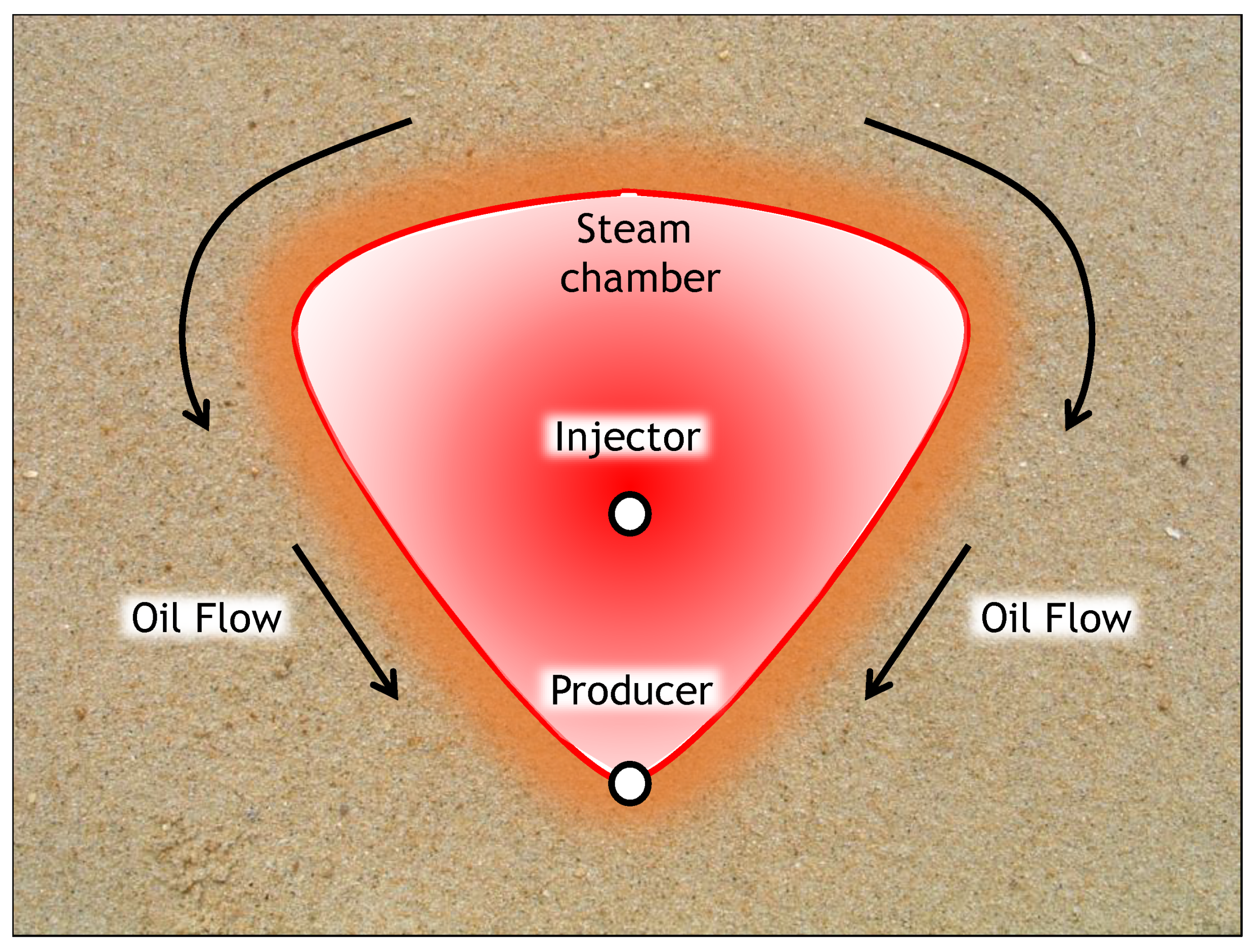
1.1. Steam Assisted Gravity Drainage (SAGD)

In SAGD, steam is injected into the reservoir in such a way that it warms the oil until its viscosity is low enough for it to flow by the effect of gravity. This is accomplished by drilling two parallel horizontal wells as it is shown in Figure 1: the well that is at the top is a steam injection well and the well at the bottom is the oil producer well.
The first analytical model that was proposed to describe the performance of a SAGD process was developed by Butler in 1985 [2]. In this model the steam chamber interface is divided into a number of segments. The oil drainage is calculated for each segment and these rates are used to calculate the displacement of the interface. This calculation is repeated in a cyclic manner and the end of the process it is possible to obtain the change in oil rate as well as the change in the position of the interface through time.
Since the development of SAGD by Butler et al. [1] there have been almost 40 years of experimental and numerical studies as well as field applications. While SAGD remains an effective technique for recovering heavy oil, it consumes large amounts of energy and fresh water. Thus, reducing the consumption of energy and fresh water is an ongoing area of research. One of the many SAGD variations consists of the injection of a solvent into the reservoir, either simultaneously with the steam or in place of the steam. The diffusion of the solvent into the oil contributes to the overall viscosity reduction.

1.2. Vapor Extraction (VAPEX)

An early proposal for employing solvent injection in heavy-oil reservoirs was presented by Butler and Mokrys [3]. Their proposed process, which was called vapor extraction (VAPEX), consisted of injecting a vapor-phase solvent into the reservoir, instead of steam. The early numerical simulations showed that the addition of a solvent into the steam results in higher oil recoveries in comparison to SAGD [4,5,6,7,8]. Subsequently, lab-scale experiments were performed using propane, injected just below the dew point, and it was seen that the results were comparable to those obtained with SAGD [9]. The authors also observed that the produced oil contained a reduced amount of asphaltenes at the end of the process [9].
In a later study, Das and Butler [10] performed experiments with VAPEX in a sand pack model as well as in a Hele–Shaw cell using butane and Peace River oil. The authors observed that the oil recovery in the sand pack model was 3 to 5 times larger than what was observed in the Hele–Shaw cells. In addition, they observed that, due to the physical properties of the sand pack, the oil production in the sand pack model deviated from the one predicted by the analytical model proposed by Butler and Mokrys [3]. According to Boustani and Maini [11], the discrepancy between these results can be reduced if dispersion is taken into account in the mass transfer model of VAPEX. The authors [11] proposed using an effective diffusivity rather than the conventional molecular diffusion coefficient.
It has been shown that the reservoir temperature has an important effect on the performance of the VAPEX process [12]. A temperature increase of only 5 °C can lead to an increase of 3% in the oil recovery factor [13]. This is because the solubility of the solvent increases at high temperatures. For this reason, VAPEX tends to perform better in reservoirs with high initial temperatures. From an operational point of view, the VAPEX process showed promising performance in terms of the final cumulative oil recovery, and a lower energy overall energy consumption. However, the high cost of the solvents prevented the VAPEX process from being implemented on a wide-scale.

1.3. Expanding-Solvent Steam Assisted Gravity Drainage (ES-SAGD)

Given the previously noted benefits of solvent injection, several authors have investigated schemes that combine steam and solvent injection. The first study to examine the effect of injecting solvents in conjunction with steam was the numerical study performed by Shu and Hartman [14]. In their study, the co-injection of solvent with steam creates a transition zone of low viscosity between the steam and the heavy oil. The vaporized solvent travels with the steam and then condenses in the cooler regions of the reservoir, which subsequently improved the effect of viscosity reduction by heat transfer. The results from the numerical simulations showed that the process was highly dependent on the solvent that is injected. The solvents were divided into light, medium, and heavy according to their volatility. The medium solvents (C6–C12) led to the best improvement in the final recovery.
Zhao [15] subsequently proposed a recovery process called steam alternating solvent (SAS), which consists of alternating the injection of steam and solvent. In SAS the process starts in the same manner as SAGD until the heat losses to the overburden become significant. At that moment, the injected fluid is switched to a solvent, until the chamber temperature is reduced. This cycle is repeated until it is no longer economical to continue, taking into account the amount of solvent retained in the reservoir and the steam–oil ratio. In their study, Zhao [15] used numerical simulations to analyze the process and concluded that the production rate that is achieved with SAS could be as high or higher than that of SAGD process while the energy input per unit of oil recovered is 18% less than SAGD. Zhao [15] also noted that the performance of SAS is highly dependent on the duration of the steam and solvent injection periods.
In 2003, Nasr et al. [16] proposed the name expanding-solvent steam assisted gravity drainage (ES-SAGD) for processes in which steam and solvent are injected together. The main purpose of this variation is to reduce the amount of steam that is being used and at the same time to further reduce the bitumen viscosity, via the diffusion of solvent into oil. Nasr et al. [16] tested the process in laboratory experiments in which the co-injection of steam with condensable hydrocarbon solvents, propane (C3) to octane (C8), was compared with the injection of pure steam. The experiments showed that the two factors which most strongly affected the feasibility of the process were the amount of solvent that is added to the steam and the amount of solvent that is recovered at the end of the process.
Dittaro et al. [17] reported the results of a pilot project conducted at Cold Lake, Alberta, Canada, in which solvent (diluent) at 20% concentration (volume) was injected with steam in an ES-SAGD process. The oil rates increased from 40 to 75 m3/day and the instantaneous steam-oil ratio (SOR) was maintained at a value between 3 and 4. In this project, the solvent recovery at the end of the process was more than 75%, which agreed with the results from the scaled physical experiments and numerical simulations that were previously performed by the same authors.
In 2007, Gates [18] performed numerical simulations to analyze the performance of the co-injection of hexane with steam (ES-SAGD) into a heterogeneous heavy oil reservoir. His results forecasted a 50% improvement in the cumulative oil production after eight years, when compared to SAGD. Additionally, the ES-SAGD process showed a higher energy efficiency, in terms of the net injected energy to oil ratio. According to the obtained results, the energy savings using ES-SAGD can be as high as 3 GJ for each cubic meter of produced oil, which can be translated into an important amount of natural gas that is saved for other projects. One of the most interesting observations of Gates [18] is how the performance of the ES-SAGD process changes with the operational conditions. In a SAGD process, saturated steam is injected, and thus the temperature of the steam is fixed, for a given injection pressure. By contrast in an ES-SAGD process the addition of a solvent, or solvents, will increase the system’s degrees of freedom in accordance with the Gibbs Phase Rule [19]; this implies that both the temperature and pressure can be independently varied in an ES-SAGD process. Gates [18] noted that while the steam became more effective at reducing the oil viscosity as the temperature increased, the solvent became less effective at reducing the oil viscosity as the temperature increased. The latter observation is due to the solubility of solvent in oil decreasing as temperature increases. Thus, Gates [18] noted that the optimum operating conditions are those which balance the effect of both the steam and the solvent, on the viscosity.
Govind et al. [20], in 2008, performed a numerical sensitivity study of ES-SAGD considering the important operating variables, as identified in previous studies [18]. They used a numerical simulation model to test the performance of butane, hexane, pentane, heptane, and a mixture of hexane–octane. One of the conclusions was that higher solvent concentrations for all these solvents as well as higher injection pressures accelerated the oil production. Nevertheless, if the solvent that is being used is considered expensive in relation with the oil, then the amount of recovered solvent must be taken into account.
Sharma et al. [21] numerically studied the addition of a small amount of non-condensable gas into the injected steam in a SAGD process. They derived an analytical model and compared it against the results of numerical simulations, which were also part of their study. In this study, methane was used as the non-condensable gas. The results showed that the methane co-injection is generally unfavorable for a SAGD process. This was said to be because the methane tends to accumulate at the steam condensation front. Thus, the heat transfer of the steam to the oil is reduced, which results in lower oil rates and a slower movement of the interface.
In 2013, Edmunds [22] presented a computational study in which they investigated the effects, on ES-SAGD, of varying the solvent concentration and the temperature and pressure at the injector. This study showed that changes in the oil viscosity are affected by the type of solvent that is mixed with the steam. The pressure-volume-temperature (PVT) properties of this mixture, which are related to the concentration of solvent in the steam, modify the system’s bubble point temperature which in turn alters the performance of an ES-SAGD process. Regarding the solvent selection, it was mentioned that the choice of solvent depends on the expected operating pressure since this pressure will lead to a different saturation temperature for each solvent. Finally, Edmunds mentioned that a heavier solvent is generally preferable for low-pressure operations.
The relation between the ES-SAGD performance and the steam–solvent PVT properties (solvent type and concentration and reservoir conditions) was also experimentally and numerically investigated by Khaledi et al. [23]. It was observed that the azeotropic behaviour of the steam–solvent mixture is highly related to the temperature changes at the boundary of the steam chamber. This temperature, which could be significantly lower than the injection temperature, affects the thermal efficiency of the process as well as the bitumen drainage rate. The authors also noted that light solvents can negatively impact the results an ES-SAGD process when it is performed at low operating pressures.
The performance of an ES-SAGD process was analytically modeled by Rabiei [24] in 2017. In this study, an unsteady-state semi-analytical model was developed to calculate the oil rate in an ES-SAGD process. This model was based on the original SAGD model from Butler and it was validated against numerical simulations as well as experimental results from physical-model tests. The results from the analytical model showed an enhancement in the oil production for cases of ES-SAGD in which different solvents were added to the steam.
The effect of reservoir heterogeneities on the SOR was numerically investigated by Venkatramani and Okuno [25]. They observed that the dilution of bitumen by solvent is more significant in reservoirs that contains permeability barriers that limit the flow in a SAGD process. In these situations, the expected increase in SOR is counteracted by the enhancement in the oil flow due to the presence of the solvent. In this research, the authors analyzed the ES-SAGD process with hexane using numerical simulation and a SAGD analytical model.
Recently, Eghbali and Dehghanpour [26] analyzed the ES-SAGD process with butane and propane using numerical simulation. Their results showed that the increase in the oil rate due to the solvent injection is reduced and eventually stabilized as more solvent is injected with the steam. This was attributed to water that condenses and accumulates at the bottom of the chamber and reduces the contact area between the condensed solvent and the heated bitumen. According to the authors, a possible way of enhancing the performance of an ES-SAGD process is to design a co-injection strategy with a reducing trend of solvent concentration versus time.
The economic feasibility of the ES-SAGD process is highly dependent on the properties and the price of the solvent. This was shown by Gupta et al. [27] in a study in which they described a field pilot test of ES-SAGD. They concluded the final net present value (NPV) was highly dependable on the solvent price and solvent retention. One of their final remarks was that even though the production is increased substantially in an ES-SAGD process, the economic enhancement cannot be generalized because it strongly depends on the amount of solvent that is recovered. According to Gupta et al. [27], an ES-SAGD process tends to have solvent recoveries of approximately 75% [27]. In many cases the cost of the solvent that is used can be significantly higher than the oil price, which could affect the economics of the project. Gates [28] also noted that in terms of energy efficiency, an ES-SAGD process is better than SAGD because the net injected energy to oil ratio (cEOR) is lower for ES-SAGD. According to Gates, the energy savings by using ES-SAGD can be as high as 3 GJ/m3 produced oil, which corresponds to 78 m3 of natural gas saved per m3 of oil produced. In a different study, Gates [28] also shown that there is a proportional relation between the steam–oil ratio (cSOR) and the amount of CO2 emitted per m3 of oil. This means that for a process that is using less steam such as ES-SAGD, it is expected to obtain a lower amount of CO2 emissions.

1.4. Cyclic ES-SAGD

Rather than continuously injecting steam and solvent, as in ES-SAGD, cyclic ES-SAGD [29] is a process that consists of alternating periods of injecting pure steam and injecting solvent plus steam. During the latter periods, the injection would have the same characteristics as an ES-SAGD process, and when these solvent co-injection periods finishes, then the process would behave as SAGD. While cyclic ES-SAGD has not yet been implemented at the field scale, preliminary numerical simulations have shown promising results.
In 2008, Gates and Chakrabarty [30] used a genetic algorithm coupled with a numerical simulator to determine the best injection strategy in an ES-SAGD process in terms of the cumulative net energy to oil ratio. In this study, unlike the studies in the previous section, the solvent concentration varies with time in a cyclical manner. However, while the solvent concentration varied cyclically with time it never went to zero. The injection pressure and the solvent concentration in the steam were modified in multiple runs in order to determine which combination generates the lowest energy to oil ratio. Variations in these two parameters led to a wide range of results which provided evidence of the importance of the injection strategy in the performance of the process. One of the subsequent conclusions of this work was that the solvent that is added to the steam should not be in excess, but just enough to supply heat and solvent to the bitumen layer at the edges of the steam chamber. This means that an ES-SAGD process could be improved if the solvent concentration in the steam is not always constant but changing through time during the process.
Manfre Jaimes et al. [29] recently performed a rigorous numerical simulation of the cyclic ES-SAGD process, using different solvents, cycle duration, and solvent concentrations. Their results showed that intermittent injection of solvent with steam could achieve similar results as a continuous solvent–steam injection while increasing the energy efficiency of the process due to the reduction in the solvent retention in the reservoir. In their simulations seven solvents were tested (C1, C2, nC3, nC4, nC5, nC6, and CO2) and it was forecasted that hexane was the solvent that led to the greatest cumulative oil production after 10 years. Additionally, it was predicted that the use of the non-condensable hydrocarbon solvents (C1, C2, and nC3) and CO2 would not yield significant improvements in the cumulative oil recovery after 10 years of production.
To date, the studies of Gates and Chakrabarty [30] and Manfre Jaimes et al. [29] are the only works that have investigated the feasibility of cyclic ES-SAGD processes. However, both of those works were rigorous numerical studies and neither of them presented an attempt to correlate the results with a simplified analytical model. Analytical models are not intended to replace rigorous numerical simulations, rather their relative ease of implementation makes them appropriate for the design of subsequent rigorous numerical simulations; a single numerical simulation may require hours or days of computing time whereas analytical models can provide their estimates in a matter of seconds. In addition, the use of analytical models is not restricted by costly software licenses. Thus, analytical models are a valuable tool that can be used to rapidly provide an order of magnitude estimate of a process’ performance. In this study, an analytical model that can be used to approximate the oil production rates and the cumulative oil production in a cyclic ES-SAGD process is presented. The organization of the manuscript is as follows: The theory section will review the necessary components of the models of Butler [2] and Rabiei [24] before subsequently discussing how these two models can be combined for analyzing cyclic ES-SAGD processes. The ensuing results section will be divided into three sections. In the first section, the performance of Butler’s model [2] and Rabiei’s model [24] will be evaluated. Subsequently, the cyclic ES-SAGD analytical model will be compared against the results from numerical simulations performed by Manfre Jaimes et al. [29], including the performance of hexane, pentane, and butane as the solvents. Finally, a detailed analysis of the performance of the analytical model will be presented for the case of hexane as a solvent and solvent + steam in the first interval.

2. Theory

In this section, Butler’s model for SAGD [2] and Rabiei’s model for ES-SAGD [24] are briefly reviewed. Subsequently, the new model for cyclic ES-SAGD is presented. The new model that is to be presented makes use of existing analytical models for SAGD [2] and for ES-SAGD [24], and thus these works will be reviewed in the following sections. Those who are already familiar with the models of Butler [2] and Rabiei [24] can skip to Section 2.3 with no loss in continuity.

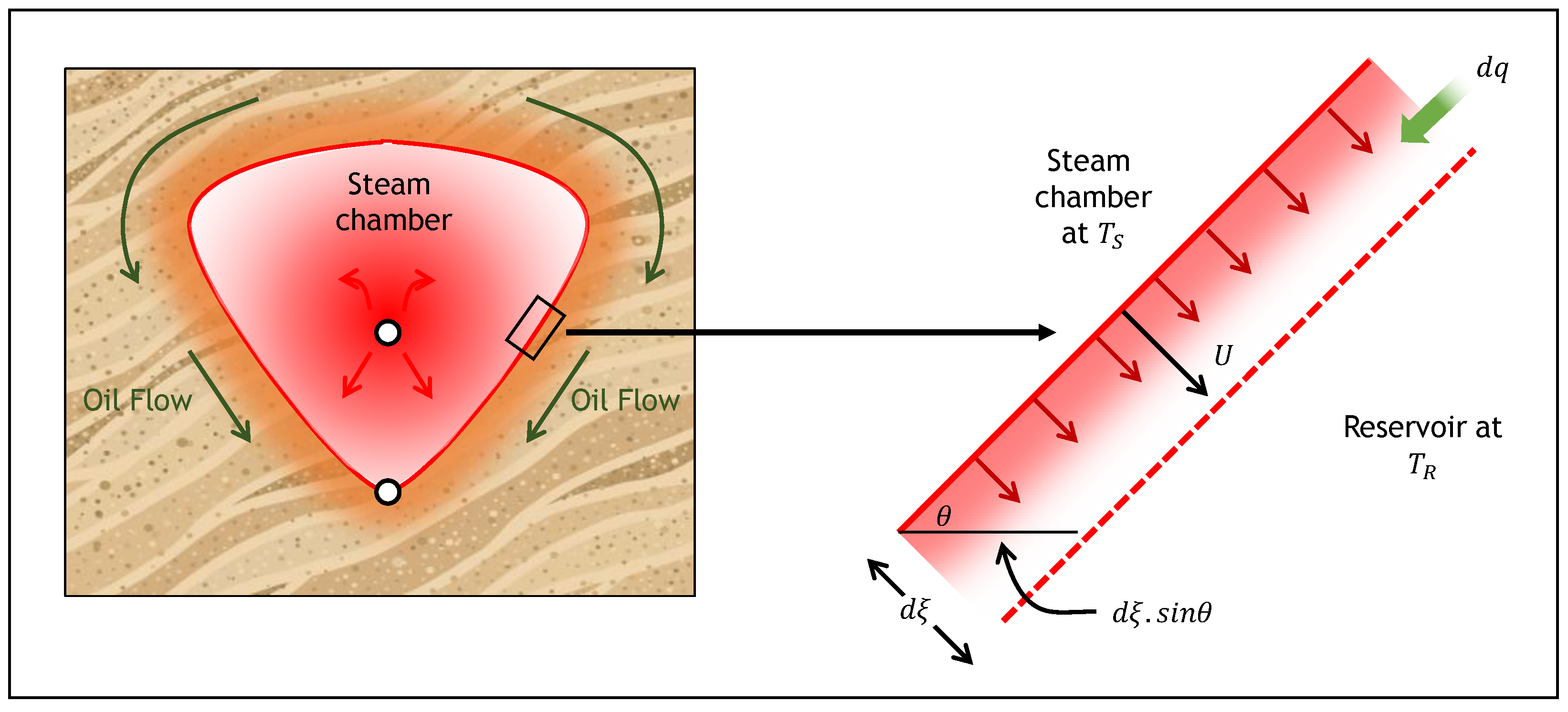
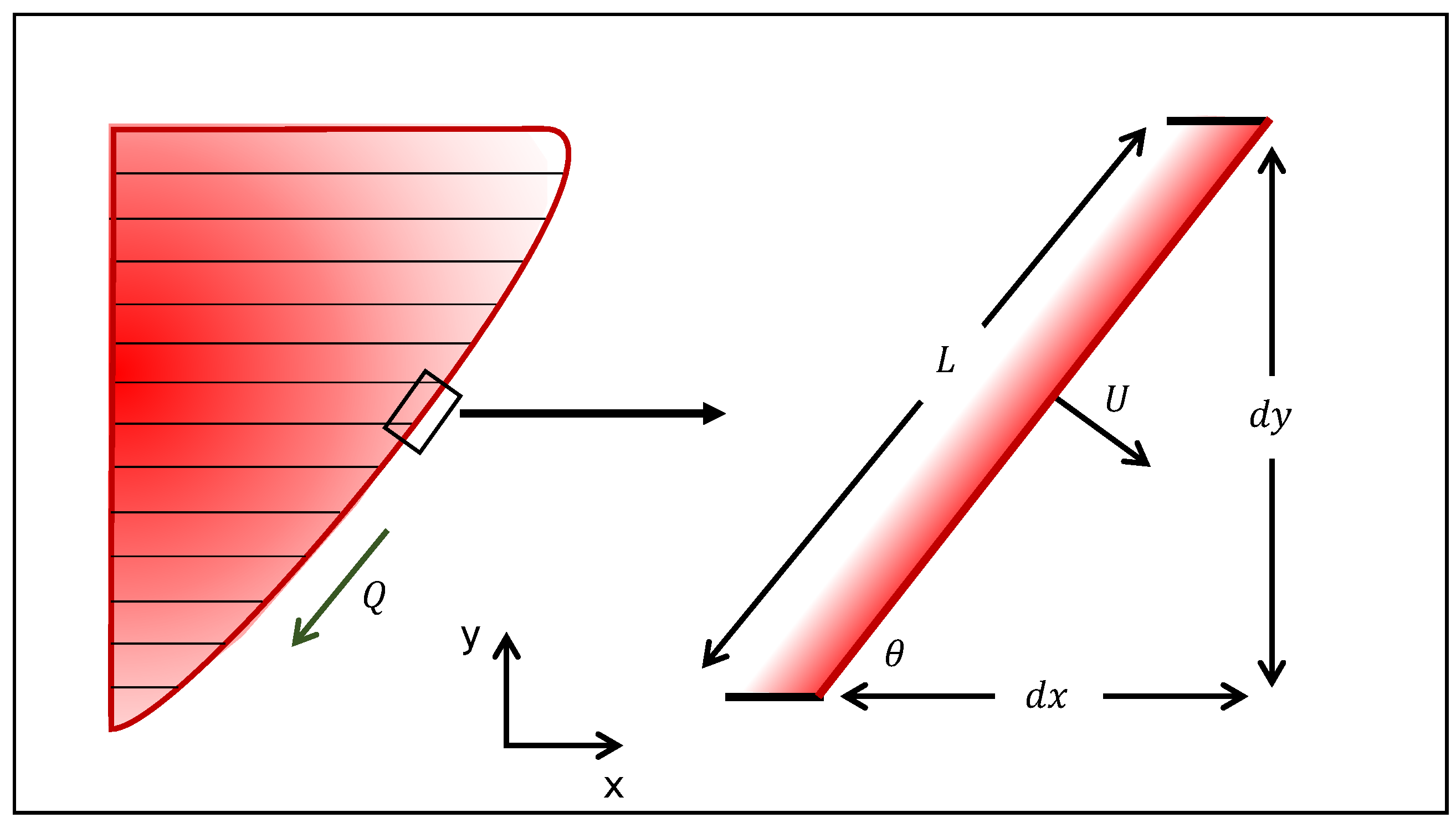
2.1. SAGD Analytical Model

In a SAGD process the temperature inside the steam chamber is assumed to be equal to the temperature of the steam ( T S ) that is being injected. This will generate a temperature gradient that goes from steam temperature at the interface until reservoir temperature ( T R ) at a particular distance from the interface. If this temperature is known, then it is possible to estimate the change in oil viscosity due to the change in temperature. In his studies [2,31], Butler showed that the change in temperature for a moving steam chamber interface can be modeled with Equation (1) which takes into account the time and distance from the interface.
T D = T T R T S T R = e U . ξ α .
The main goal of Butler’s SAGD analytical model was to describe the spreading steam chamber and to find an expression for the oil rate. Figure 2 shows a small cross section of a reservoir and the steam chamber interface at a given instant during the SAGD process. It is assumed that at that moment, the steam chamber has not spread completely in the reservoir and there is a significant volume of the reservoir that has not been heated by the steam. The steam chamber interface is moving at a velocity U. The temperature at the chamber is considered to be the steam temperature, T S , whereas the temperature at some distance from the chamber interface is equal to the original reservoir temperature, T R . The angle θ is measured with respect to the horizontal and represents the interface angle that is changing according to the interface movement. At a distance ξ, measured normal to the chamber interface towards the reservoir, the oil has a kinematic viscosity of ν. This viscosity decreases with ξ; the closer to the interface, the higher the temperature and the lower the viscosity.
In order to model the oil drainage rate and the movement of interface, Butler [2] divided the steam chamber into multiple horizontal elements, as shown in Figure 3. These elements can increase or decrease in length and in this form the movement of the steam chamber interface is approximated. The growth behaviour of the steam chamber and its interface consequently advance, in the model; these factors also affect the oil drainage rate behavior. In Butler’s SAGD model [2], the dimensionless oil drainage rate is calculated using the following equation:
q o , D = γ T . B 3 . s i n θ ,  
where γ T represents the dimensionless heat penetration depth, θ is the angle between the segment of the interface at each element and a horizontal line, and B 3 is a dimensionless number that takes into account the reservoir and fluid properties and is defined as
B 3 = k . g . H α . ϕ . Δ S o . m . ν S   .
In the calculation of B 3 , k is the reservoir permeability, g is the acceleration of the gravity force, H is the reservoir height measured from the production well to the top of the reservoir, α is the reservoir thermal diffusivity, ϕ is the reservoir porosity, Δ S o is the initial oil saturation, m is a coefficient that depends on the oil properties, and ν S is the kinematic oil viscosity at the steam temperature.
The use of the heat penetration depth allowed for the assumption of a non-steady temperature distribution ahead of the steam chamber interface, which was one of the limitations of Butler’s previous models [2]. The heat penetration depth was computed according to the following equation:
d γ T d t = 2 π ( α γ T U )   .
In the above analytical model, Equations (2)–(4) were solved for q O , D using an explicit iterative procedure with small time steps. During the iterative procedure, the thermal penetration depth at the previous time step is used as an initial guess for the penetration depth at the current time step. This procedure starts with the division of the total height of the model into a finite number of elements, as is shown in Figure 3. This procedure allows one to calculate the oil rate, cumulative production, and the movement of the interface.
The elements in which the steam chamber is divided are constantly expanding as the process proceeds. The upper elements will move faster than the lower ones and eventually, the element at the uppermost element will reach the model boundary. This situation may represent the moment where the steam chamber reaches the reservoir boundaries, or it may be due to the steam chamber coming into contact with the steam chamber from an adjacent well pair. This situation is represented by an additional step in the calculation in which the model is divided into equally spaced elements in the horizontal direction once the top element has reached the boundaries as it is shown in Figure 4. Depending on the direction of the movement, the elements’ location is calculated using Equations (5) and (6) as explained by Butler [2].
( q o , D y D ) = ( x D t D )
( q o , D x D ) = ( y D t D )

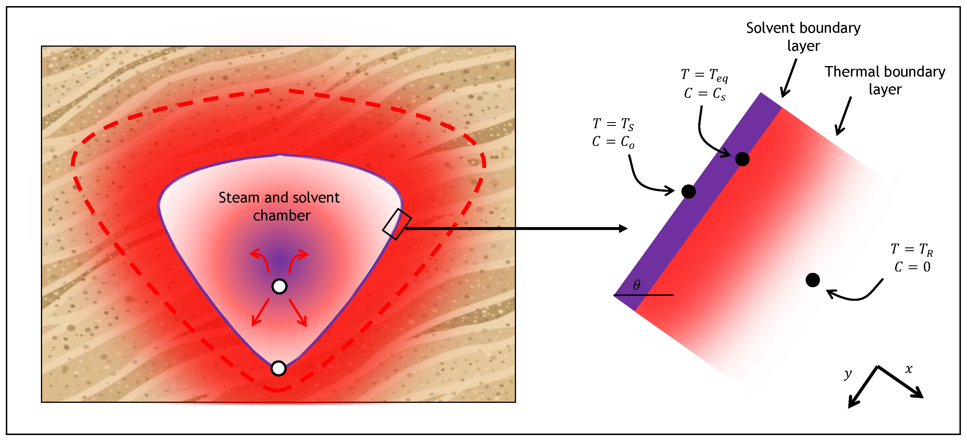
2.2. ES-SAGD Analytical Model

In an ES-SAGD process, the steam temperature and concentration of the co-injected solvent affects the behavior of the steam chamber and its interface, and it has been shown that the temperature at the interface is in turn influenced by the steam–solvent azeotropic behavior [23]. The addition of solvent in the injected stream will lower the saturation temperature of the mixture which consequently will also reduce the temperature of the steam chamber. Thus, in an ES-SAGD process, this temperature cannot be assumed to be equal to the interface temperature as it is in SAGD.
As the steam starts to condense in zones that are distant from the injection point, the concentration of steam in the injected mixture will start to decrease while the solvent mole fraction, in the vapor phase, increases. This process will continue until an equilibrium point is reached in which the temperature of the mixture is the lowest possible at which a vapor phase can exist at the injection pressure. This point also represents the lowest possible steam concentration in order to keep the mixture in the vapor phase. Thus, for a given injection pressure, the temperature at the interface in an ES-SAGD process will be lower than the interface temperature in a SAGD process. Additionally, in an ES-SAGD process, the solvent concentration at the interface will be higher than the concentration at the injection point. This situation affects the drainage rate and the thermal efficiency of the process.
As heat is transferred from the injected fluid to the reservoir, the steam temperature begins to decrease, and condensation occurs. This will in turn increase the solvent mole fraction in the mixture until it reaches a saturation temperature below which only two liquids phases (solvent and water) are at equilibrium. Figure 5 shows the phase boundary for mixtures of water and hexane, pentane, and butane at 2.5 MPa. It can be seen that these temperatures can differ considerably. For example, in a steam–pentane mixture in which the concentration of pentane is 10% mole, the dew point temperature at 2500 kPa is 217.6 °C. This temperature is less than the dew point temperature of pure steam at the same pressure: 223.6 °C. However, as the solvent concentration increases, at a constant pressure of 2500 kPa, the temperature can fall as low as 158.3 °C. In addition to this, the solvent concentration at the interface is also changing during the cycles. Thus, for the same steam–pentane mixture the pentane mole fraction and temperature at the interface are 0.803 and 158.3 °C, respectively. If the temperature at the interface subsequently starts to increase during the steam cycle, then this solvent concentration will be reduced accordingly.
Similar to Butler [2], Rabiei [24] developed a semi-analytical model of the ES-SAGD process using an unsteady-state temperature and solvent concentration distribution. The calculation procedure of this model predicts the oil flow rates and interface profile in an iterative fashion, similar to the SAGD model that was previously derived by Butler [2]. For the temperature distribution ahead of the interface, Rabiei [24] used the same model that was defined by Butler, but derived an expression for the concentration distribution using the heat integral method (HIM). The final expression for the oil drainage rate has a similar form to Butler’s but contains an additional variable, which depends on the solvent properties.
To describe the solvent concentration, Rabiei [24] applied Fick’s law in the x-direction in a small element of the interface, as shown in Figure 6. The result was
x [ ( D + κ t U ) C x ] = C t .
In the previous equation, D represents the effective solvent–bitumen molecular diffusion coefficient, C is the solvent concentration in the bitumen, and κ t is the transverse dispersivity factor. Before reaching the interface, the concentration increases starting from its initial value at the injection point, C o . Subsequently, in Equation (7), it is assumed that the solvent concentration changes from a maximum value at the interface, C s , to zero at some distance ahead in the reservoir. As seen in Figure 5, the maximum concentration value is associated with an equilibrium temperature, T e q and depends on the type of solvent and its initial concentration in the injected mixture. It is important to note that in the model of Rabiei [24], the value of C s is deduced from the steam–solvent phase equilibrium; it is subsequently used to model the maximum solvent concentration in the bitumen. The assumption that the maximum solvent concentration in the bitumen is equal to the maximum solvent concentration in the steam is only applicable in the interface [24].
Rabiei [24] developed the following approximation for the un-steady state solvent distribution in a moving boundary:
C D = e x p ( ξ D γ C , D ) ,
where C D is the dimensionless concentration, defined with respect to the concentration at the interface: C D = C / C s , and γ C , D   is the dimensionless solvent penetration depth normalized with the height of the reservoir: γ C , D = γ C / H . This value is calculated through the following ordinary differential equation:
γ C , D t D = 1 γ C , D ( 1 L e . B 3 + κ t , D . P e ) P e .  
In this expression, L e represents the Lewis number which is a dimensionless value that is defined as the ratio of thermal diffusivity to mass diffusivity:   L e = α / D . The parameter κ t , D represents the dimensionless transverse dispersivity factor normalized with the height of the reservoir, i.e., κ t , D = κ t / H . In Equation (9), the initial condition is γ c , D = 0 at t D 0 . This equation is solved numerically at each time step to determine the solvent penetration depth.
To model the change in viscosity due to the combined effect of heat and solvent concentration, Rabiei [24] derived an expression that combines Butler’s [2] correlation for temperature-dependent viscosity and Shu’s [33] correlation for solvent concentration-dependent viscosity:
ν m i x ν o   a t   T S = ( ν s   a t   T S ν o   a t   T S ) x s T D m .
This expression takes into account the oil and solvent kinematic viscosities at steam temperature, ν o   a t   T S and ν s   a t   T S and an exponent x s that is calculated through:
m = x s m s + x o m o .
In this equation, m o and m s are the viscosity exponents for the oil and solvent, respectively, while x s and x o are calculated in a similar way as was defined by Shu [33]:
x s = C s C D α s + ( 1 α s ) C s C D .
x o = 1 x s ,
where α s is a parameter defined by Shu that depends on the specific gravities and viscosities of the two fluids in the mixture.
Taking into account the change in the oil rate due to the combined effect of the heat and mass transfer, Rabiei [24] proposed the following expression to describe the oil rate in an ES-SAGD process:
q o , D = B 3 . s i n θ . γ T , D . q R   .
The previous equation is similar to the one derived by Butler [2] save for the factor q R , which is calculated using the following expression:
q R = m o 0 1 ( ν o ν s ) x s T D m 1 [ 1 C s . T D ( γ T , D γ C , D ) ] d T D .
where T D is the dimensionless temperature and γ T , D and γ C , D are the dimensionless heat and solvent penetration depths. This integral was evaluated using numerical quadrature.

2.3. Cyclic ES-SAGD Analytical Model Description

The cyclic ES-SAGD process is modelled by considering it to be a combination of SAGD and ES-SAGD. During the steam injection cycles the temperature at the interface corresponds to the steam temperature at saturated condition while, during a solvent–steam cycle, the interface temperature is lower since it corresponds to the equilibrium temperature between the steam and the solvent at the maximum solvent concentration.
The first stage of the Cyclic ES-SAGD model behaves as either pure SAGD or pure ES-SAGD, depending on the injection sequence. After this first cycle, an additional step is included in the process in which the interface temperature is computed for each element, at each time step. This computation will directly affect the subsequent oil drainage rate of the process. The change of temperature at the interface will depend on the time that has elapsed since the steam or steam–solvent cycle started and the distance between the interface and the injection wells. To estimate a value for the temperature change at the interface, Equation (16) was applied after the change in cycles. This equation represents an unsteady-state temperature distribution for a semi-infinite one-dimensional element with a known temperature imposed in one of its sides that generates a temperature gradient which changes over distance and time [34]. In addition, Equation (16) assumes that the thermal diffusivity (α) is constant and that the vertical dimension in each element is negligible in comparison to the horizontal dimension. This is a reasonable assumption taking into account the shape of the elements in which the steam chamber is divided.
T D = e r f c ( x 2 α t )   .
For the cycles which consist solely of steam injection, the temperature at the interface will affect the viscosity of the oil and its drainage rate. To compute the oil rate, Equation (2) was modified using the new oil viscosity at the steam temperature as shown in Equation (17). In this expression, ν T s is the kinematic oil viscosity at the steam temperature which was used to calculate the constant B 3 and ν T i n t e r f is the kinematic oil viscosity at the interface. This equation is substituting the previous viscosity value with the new viscosity that is considering the temperature change in the interface. The oil drainage rate is directly proportional to the ratio of these viscosities. Initially, the low interface temperature in the steam + solvent cycles will reduce the rate but as the temperature increases the rate will increase until it reaches the value it would have had if the steam injection would not have been preceded by a solvent–steam injection.
q D = q D ν T s ν T i n t e r f   .
For the steam–solvent cycles, the change in the interface temperature will affect the calculation of q R . According to Equation (15), q R depends on the oil and solvent viscosity at steam temperature. These viscosities are calculated for each element depending on the interface temperature. Additionally, the equilibrium solvent concentration at the interface, C s , also changes with the temperature. In this study, the value of C s was computed with the aid of Winprop [32], which used the Peng–Robinson equation of state.
The Cyclic ES-SAGD model consists of the calculation of the oil rate and interface movements during each steam and solvent–steam cycle using the equations from the Butler’s [2] and Rabiei’s [24] models and, additionally, the calculation of the temperature and concentration change at the interface at the end of each cycle. Performing the aforementioned calculations, it is possible to analytically describe the cyclic ES-SAGD process for different solvents, concentrations and cycle lengths.

3. Results

3.1. Computational Procedure

Similar to the SAGD and ES-SAGD analytical models, the number of equations that must be solved simultaneously necessitates the use of an iterative procedure with small time steps in which the calculations are performed for all the elements at each time step. The size of these time steps must be determined in such a way that it is possible to run the routine stably. MATLAB® was used to perform the calculation procedure. Figure 7 shows a flow diagram of the computational procedure, for cases in which the first cycle corresponds to the injection of steam plus solvent. In cases where the first cycle involves only steam the solvent mole fraction, in Figure 7, can be set equal to zero. This figure will be used as a reference to what will be explained in the following paragraphs.

3.1.1. Input Data

Prior to beginning the computation, the following must be specified:
  • Reservoir properties: porosity, permeability, thermal diffusivity, and initial oil saturation.
  • Height of the model, H, measured from the production well to the top of the model.
  • Width of the model normalized with respect to the height, W D = W / L . The width of the model is considered to be half of the complete model. As it was done with the previous analytical models, the computations are performed for half of the steam chamber.
  • Total duration of the proposed cyclic ES-SAGD procedures, t e n d .
  • Duration of each injection cycle, t c y c l e .
  • Injection pressure, mole fraction, and the type of solvent that is used.
  • Start mode: this variable tells the algorithm if the initial cycle would be a steam or a steam–solvent cycle.
  • Time step size ( s t e p ).

3.1.2. Initialization

In this section, the input data was used to calculate the constant B 3 (Equation (3)). Additionally, the following parameters are defined:
  • Total number of steps ( n = t e n d / s t e p ): it depends on the step size and the length of the calculation. This variable is used as a stopping criterion for the whole procedure.
  • Steps for each cycle ( i c y c l e = t c y c l e / s t e p ): this is the number of time steps that each cycle will take.
  • Iteration counter ( i ): this variable count each of the steps that are taken in the calculation. The procedure stops when i is equal to n .
  • Initial heat (Equation (4)) and concentration (Equation (9)) penetration depths: both SAGD and ES-SAGD previous analytical models use an initial penetration depth in order to start the algorithm. In this case, both penetration depths were set to 0.01. This number was assigned after running multiple cases taking into account the convergence of the equations.

3.1.3. First Cycle

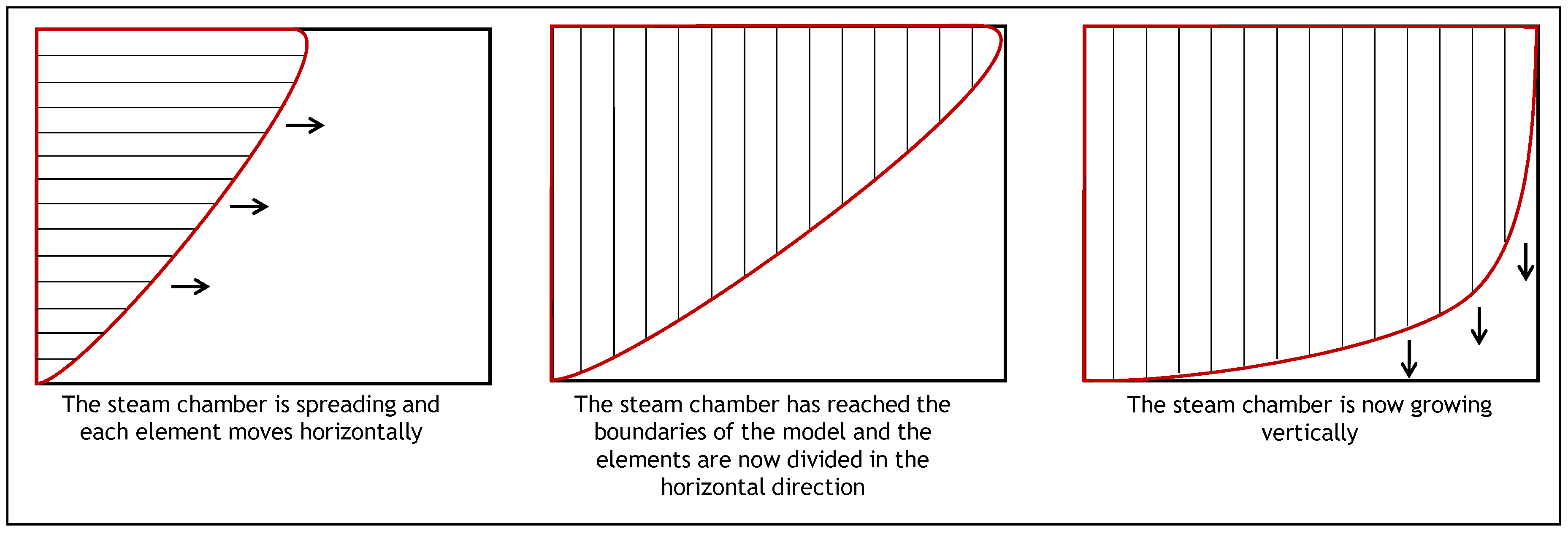
  • This part of the procedure corresponds to the calculations that are performed for the first cycle. These calculations are repeated for the number of steps of the cycles ( i c y c l e ). During this part, each element is considered for the calculation of the oil drainage rate, the movement in the horizontal direction, the angle, the velocity, and the dimensionless penetration depths. Depending on the type of injection scheme (steam or steam + solvent), the appropriate expression from Section 2 is used to calculate the rate changes.
  • At the end of each time step, the variable t stores the time at which the rest of the variables were calculated, i increases with each iteration and it represents the current step, and the variable t c h a n g e 1 stores the time at which the change of cycle will occur. This variable is used afterwards to calculate the temperature at the interface.

3.1.4. Recurrent Steam and Solvent Cycles

  • After the initial period of injection, a new cycle begins in which there is an alternate calculation of different injection schemes. The order of these calculations depends on the initial cycle. For the steam injection periods, the first step is to calculate the temperature at the interface ( T i n t e r f ). This temperature will depend on the time that has elapsed since the last cycle ( t c h a n g e 1 ) and the position of each element ( x D ). After that, the calculation is similar to what was explained previously; the rates are calculated taking into account the viscosity at the interface temperature using Equation (17) and then the rest of the variables are calculated considering the position of the top element.
  • For the steam–solvent injection periods, the temperature at the interface ( T i n t e r f ) is also the first variable that is calculated using Equation (16). Subsequently, the rates are calculated considering the oil and solvent viscosity at the interface temperature and then, the remaining variables are determined in the same way that was previously explained. It is important to point out that in this cycle the temperature at the interface is calculated considering t c h a n g e 2 , which is the time at which the previous injection period ended.
  • For each iteration that is performed, the counter i increases by one unit until it reaches n , and then the process comes to a stop. The change in the dimensionless oil drainage rate over time for the element at the bottom represents the dimensionless oil rate of the Cyclic ES-SAGD process.
The dimensionless oil rate and dimensionless time can be converted into the oil rate and time respectively through Equations (18) and (19) [2]. Additionally, the cumulative oil production can be calculated through the integration of the oil rate, as it is shown in Equation (20), while the interface movement in the horizontal and vertical direction is calculated as explained by Butler [2].
q o = q o , D . α . ϕ . S o . B 3
t = t D . H 2 B 3 . α
N p = 0 t D Q o , D d t D . H 2 . ϕ . S o
It is worthwhile to re-emphasizing that the type of solvent and its initial concentration in the steam will modify the viscosity of the mixture and the final oil rate. In addition, each solvent had a different concentration at the equilibrium temperature with the steam ( C s ) which also modifies the calculation of the oil rate. This concentration was also altered by the pressure at which the solvent was being injected which also affects the saturated temperature of the steam. From the pressure, the saturated temperature of pure steam was estimated using CMG-WinProp [32]. Knowing the pressure, the type of solvent and its concentration it was possible to calculate the equilibrium temperature with the steam ( T e q ) and the maximum solvent concentration ( C s ) through flash calculation. In this work, thermodynamic properties were computed through CMG-WinProp [32] applying the Peng–Robinson equation of state.

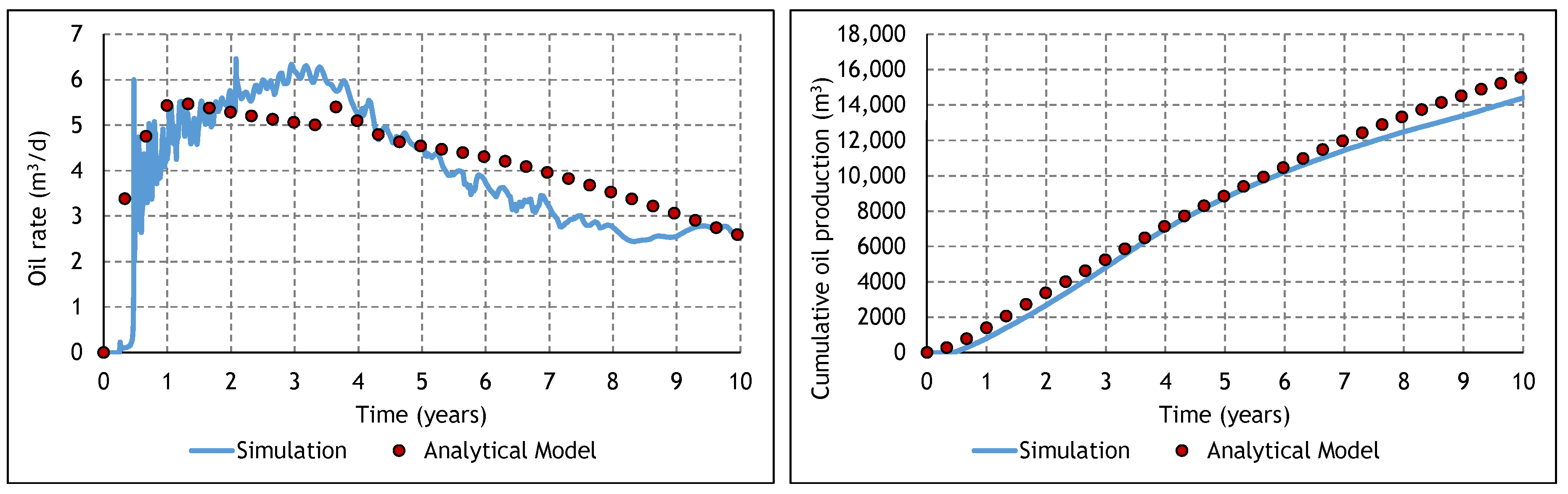
3.2. Analysis of the Constituent SAGD and ES-SAGD Models’ Performance

In the following sections, the performance of the cyclic ES-SAGD analytical model was compared to rigorous numerical simulation results. As the cyclic ES-SAGD model was a combination of existing models for SAGD [2] and ES-SAGD [24], these models’ performances are first reviewed. The purpose of including this material is to provide points of comparison for the cyclic ES-SAGD model. Readers who are already familiar with the qualitative behaviour of Butler’s model [2] and Rabiei’s model [3], can skip to Section 3.3 without loss of continuity. Finally, before presenting the numerical comparisons, it should be noted that the models of Butler [2] and Rabiei [24] have both been compared with relevant experimental data and both models were able to correlate the laboratory data [2,24].
The model in the numerical study was a representation of half steam chamber in a solvent–steam injection process and it contained two wells: an injection well with a constraint of maximum bottom hole pressure of 2500 kPa where steam with a quality of 0.8 and a production well with a constraint of a maximum steam rate of 1 m3/day. The steam temperature is used to estimate the oil viscosity at that condition which is part of the input data in Equation (3).
Table 1 shows the model parameters of the reservoir model. The reservoir was assumed to be homogeneous; hence, all the properties were assigned as a constant value to all cells. There are no aquifers or any gas cap in the model. The values that are shown in Table 1 were taken from previous numerical studies in the Athabasca region: the permeabilities, porosity, and initial oil saturation were taken from Shin and Polikar [35], the initial reservoir pressure and the thermal properties were the ones used by Rabiei [24], while the endpoints for the relative permeability curves were taken from Gates [18]. These endpoints were used in the Stone’s three phase relative permeability model that was included in the simulator that was used: CMG STARS [36].
The fluid properties, in the numerical simulator, were modeled as a live oil via the Peng–Robinson equation of state using two pseudo-components: methane with 4 mol% in the mixture and a heavy pseudo-component, which represented bitumen. The oil molecular weight was 590 g/mol, the density, 1012 kg/m3, and the saturation pressure, 3200 kPa. These values were taken from the research done by Strausz and Lown [37]. According to these authors, the previous number represent typical values for the oil that is contained in Athabasca reservoirs.
To compare the models, the input data of the analytical model related to the size of the reservoir and its properties was set to the same values as the ones used in the simulator model. A factor of 0.45 was used to represent the oil relative permeability in the analytical model. In addition, the m s and α s parameters were modified in order to match the mixture viscosity that the simulator was using and the time frame was shifted to account for the pre-heating and chamber raising periods as it was mentioned by Rabiei [24]. In the case of a pure SAGD case, the analytical model of Section 2.3 reduces to Butler’s model [2], while the case of continuous ES-SAGD the model of Section 2.3 reduces to Rabiei’s model [24].
Figure 8 shows the oil rate and cumulative oil production for a SAGD case, while Figure 9 shows the same for a case in which 10% mole hexane was continuously co-injected with steam. The initial spike in the SAGD and in the ES-SAGD cases were also observed in the simulations performed by Rabiei [24]; however, no explanation was presented. For both the SAGD and the ES-SAGD case, the oil rates predicted from the analytical model follow the same trend as the results from the numerical simulation. However, the analytical model slightly over estimates the cumulative oil production. Additionally, the analytical model over-estimates the oil production, particularly during the final years when the simulation results are showing that the steam chamber had covered most of the reservoir and the oil rate had started to decrease. The differences in the oil rate at the beginning of the process are related with the size of the timesteps that are used by the numerical simulator and the analytical model; the numerical uses an adaptive time step, whereas the analytical uses a constant time step. Additionally, the numerical and the analytical use different fluid property packages.
The discrepancies in the results shown in Figure 9, particularly for the later period, are related to the way in which the steam chamber interface moves in both scenarios; in the analytical model the steam chamber grows horizontally until it reaches the boundaries and then starts to move vertically, which is different than the interface movement in a numerical simulator. In addition to this, the analytical model and the numerical simulation have different ways of modeling the change in oil viscosity by the effect of temperature. In order to find a decent match between the analytical model and the numerical simulation is necessary to adjust the m s and α s parameters that control the oil viscosity and to match them against the results from the numerical simulation. A similar process can be used if there is experimental data available, as in the study presented by Rabiei [24].

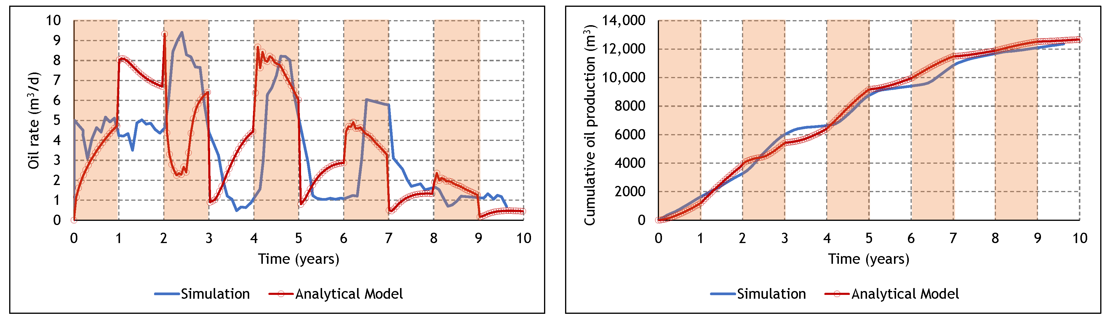
3.3. Analysis of the Cyclic ES-SAGD Model’s Performance

In this section, the cyclic ES-SAGD model is applied to the same reservoir as described in the previous section. Figure 10, Figure 11 and Figure 12 show a comparison between the numerical simulation and the analytical modeling of the cyclic ES-SAGD process, using three different solvents: hexane, pentane, and butane. In these cases, the cycles had a duration of one year and the initial cycle corresponded to a steam–solvent injection. The areas highlighted in yellow represent the periods where the steam–solvent injection took place. In all three cases, there are number of noteworthy characteristics. Firstly, upon changing between steam and steam plus solvent, the analytical model predicts a much more rapid change in the oil rate than what is predicted by the numerical simulator.
The analytical model does not account for convective heat and mass transfer or for changes in the steam quality. Additionally, Butler’s model for the SAGD cycles does not account for the presence of residual solvent in the reservoir and as a result, when the cycle changes from steam + solvent to pure steam, the analytical model implies a step change to zero solvent concentration throughout the reservoir. Thus, upon changing between steam and steam plus solvent the analytical model will predict a much more rapid change in temperature throughout the reservoir. Hence, as previously noted, the analytical model can be thought of as representing a limiting case.
A second noteworthy feature can be seen upon examination of the magnitude and direction of the change in flow rate upon switching from steam plus solvent to steam, at year 1. In Figure 10, the oil rate falls and then gradually rises, whereas in Figure 11 and Figure 12, the oil rate spikes and then slowly declines. Additionally, the spike in oil rate is greater for butane than for pentane. This behaviour can be explained by examining the oil–solvent PVT behaviour, as shown in Figure 5. At the end of the steam plus solvent cycle, the temperature in the reservoir is at or near the azeotrope temperature. Upon switching to straight steam, the temperature subsequently rises to the saturation temperature of steam, at the injection pressure. This temperature rise is roughly 50 °C when hexane is the solvent, 70 °C when pentane is the solvent, and it is almost 100 °C when butane is the solvent. This temperature difference will subsequently affect the rate of heat conduction and hence, the differences in the production profiles.
A final common feature is that the agreement of the cumulative oil production predictions is very good, although the analytical model slightly overpredicts the cumulative oil production for most of the process. Given the previous notes regarding the rate of heat transfer in the analytical model versus the numerical simulator as well as the SAGD portion of the model not accounting for residual solvent, this overprediction is expected.
To quantify the differences between the results obtained by the numerical simulation and the analytical model, both the oil rate and the cumulative oil production curves were interpolated at the same time values and then the results from each method were compared. In terms of statistically comparing the analytical results to the numerical results, the absolute relative was computed over the ten-year process. The average absolute relative errors in the cumulative oil production, expressed in percentages, were 9.5%, 8.7%, and 9.4% for the hexane, pentane, and butane, respectively. Regarding the oil rate, the maximum absolute deviation between the numerical and analytical model was 37%, 28%, and 25% for the cases of hexane, pentane, and butane respectively.
Additional insight into the proposed model’s performance can be gained by examining the predicted shape of the steam chamber. Figure 13 compares the interface position as predicted by the cyclic ES-SAGD model (black dashed lines) with that of the numerical simulation result. Figure 13a shows the steam chamber location at the instant that the analytical model reaches the boundary whereas Figure 13b shows the steam chamber at a later time point in the simulation. As was also observed in the model of Butler [2] and Rabiei [24] the shape of steam chamber predicted by the analytical model is different from the numerical results at early times in the simulation, whereas at later times the two profiles are much more similar in shape and location. Rabiei [24] attributed this difference to “an extensive horizontal expansion of the chamber as result of enhanced flow rate by solvent addition; therefore, as the chamber reaches the top of the formation, the higher flow potential is used to drain oil along the elongated interface towards the production well.” [24]. The authors of the current study, however, believe that the difference in the shape of the steam chamber at early times in the simulation is an indication that convective heat transfer is prominent during the initial stages of the simulation. The importance of convection, in ES-SAGD processes, was also noted by Keshavarz [38], who observed that “From an analytical modeling perspective, however, neglecting the contribution from convection to the mixing process at medium to high temperatures will require diffusion and/or dispersion coefficients that are orders of magnitude larger than the experimentally measured values in order to obtain comparable drainage rates”.

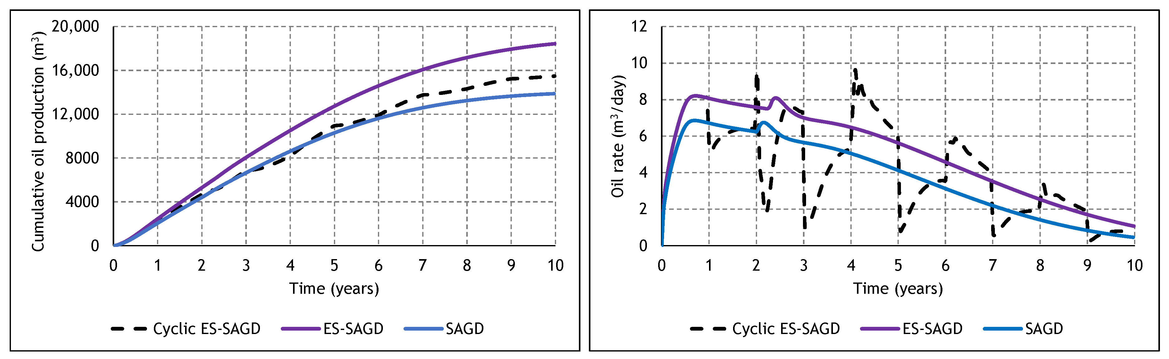
3.4. The Effect of Cycle Length and Starting Mode

In the previous section, the analytical model’s performance was assessed with three different solvents. In this section, a more detailed comparison of cyclic ES-SAGD with SAGD and ES-SAGD will be presented. Additionally, the effect of cycle length and starting mode are examined. The results in this section are limited to processes that use hexane as a solvent; in the previous numerical simulations, Manfre Jaimes et al. [29] determined that hexane was the optimal solvent. Hexane is also the solvent that most closely approximates the properties of the diluent that is used to transport the bitumen through pipelines [18]. Table 2 summarizes the parameters that were used in this calculation, which was performed dividing the steam chamber in 20 elements. The diffusion coefficient for hexane in oil was taken from the experiments performed by Salama and Kantzas [39].
Figure 14 compares the performance of a cyclic ES-SAGD process, in which hexane was being co-injected with steam at 2500 kPa and 10% mole fraction to that of SAGD and ES-SAGD, at the same conditions. In Figure 14, it can be observed that during the last year, the oil rate from the ES-SAGD process was almost always higher than the one that was obtained from a cyclic ES-SAGD process. This difference is related to the amount of oil that was left in the reservoir at that moment due to the previous oil rates. During the first four years, the oil rate for ES-SAGD was higher than the one in cyclic ES-SAGD. This is also reflected in the cumulative oil produced during that period. At the fourth year, the steam chamber in ES-SAGD had already covered an important portion of the reservoir, whereas in cyclic ES-SAGD there were still some areas that had not been affected by the process. When the steam–solvent injection started at the fourth year for the cyclic ES-SAGD process, the oil that was left was contacted by the steam–solvent mixture, and the oil rate increased. This is an indication of the effect that the timing of the steam–solvent injection periods had on the final results as it was shown by Manfre Jaimes et al. [29].
Regarding the cumulative production, it can be seen how each cycle was affecting the slope of the curve, which was clearly related to the oil rate increments and decreases. The cyclic ES-SAGD final cumulative production at the end of the process was higher than the one obtained with SAGD, but less than the one that came from any of the ES-SAGD cases. Ultimately, the costs of steam and solvent plus the price of oil would dictate which of these three processes is preferable, at any given moment in time.
Figure 15 shows the position of the steam chamber after 1, 2.5, and 5 years for the (a) SAGD case, (b) the ES-SAGD case with 10% mole hexane injected at 2500 kPa, and (c) the cyclic ES-SAGD case with the same solvent configuration and yearly cycles, respectively. In all plots, both axes represent the dimensionless distance in the vertical and horizontal direction. As expected, it can be seen that the interface reaches the model boundary at different times for each of the three scenarios. After one year the solvent cases were significantly closer to the boundary than the SAGD case in which the boundary was reached at 2.5 years approximately. At this time, the shapes of the curves in the ES-SAGD and Cyclic ES-SAGD were considerably different because the cyclic case had gone through one year of steam injection and half a year of solvent–steam injection after the initial cycle. The lower part of the interface seemed to behave more like the ES-SAGD curve while the rest of the interface was more similar to the SAGD case. At 2.5 years the continuous solvent case curve started to flatten, which was the same effect that the cyclic case curve had at the lower part of the chamber. This effect was related to differences in the interface temperature. As mentioned previously, this difference is more pronounced at the bottom of the interface where the proximity between the interface and the injected steam leads to sharper changes in temperature and concentration. Regarding the curve which represents the interface after five years, the ES-SAGD case showed a chamber that covered almost all the model, while the SAGD case still had half of the initial area to cover. This was reflected in the oil rate and cumulative production graphs presented previously. What Figure 15 shows, agrees with the oil rate behaviour shown previously in Figure 14. The continuous steam–solvent injection in ES-SAGD led to a higher cumulative oil production at the end of the process because the steam chamber was able to cover a bigger area of the reservoir. The steam chamber in a SAGD process will eventually cover a similar area to the one that the ES-SAGD steam chamber is covering. However, it will take a longer time since the oil viscosity reduction, due to effect of the steam, is less than the reduction due to the combined effect of solvent and steam. The reduction in the oil viscosity will affect the speed in which the oil moves in the interface, and hence the speed at which the interface advances in the reservoir.
The length of each cycle as well as the starting mode are also important in assessing the performance of the cyclic ES-SAGD process. As it was previously noted, the time that elapses between one cycle and the other will affect the increase or decrease in the interface temperature that has a direct impact on the rate. Figure 16 shows the oil production rate and cumulative production for a cyclic steam–solvent injection of hexane at 10% mole using cycles of half a year, one year, and two years. There are considerable differences among the results even though the total amount of time in which the solvent was co-injected is the same for two of the cases (1-year cycle and 0.5-years cycles) and varies for the other case in a year. These differences were also observed in the numerical simulation study performed by Manfre Jaimes et al. [29]. This means that the order in which each cycle takes place has a significant impact on the performance of the process, and hence the final oil production.
Figure 17 compares the effect of the starting mode for the cyclic ES-SAGD process (i.e., steam + solvent or pure steam). Although both cyclic cases result in a cumulative production that is less than the continuous solvent case, their differences illustrate how the moment in which each cycle takes place affects the result. If it is desired to reduce the amount of solvent that is being used even though it means affecting the final oil production, then it is important to consider not only how much solvent is going to be injected but also when this solvent is going to be injected. As was shown in Figure 15, the shape of the steam chamber depends on the type of injection that is taking place. Starting with steam or steam–solvent injection will change the shape of the steam chamber at the beginning of the process which will in turn alter the way in which this steam chamber keeps growing during the whole injection period.

4. Conclusions

As a first attempt at creating an analytical model for cyclic ES-SAGD processes, the existing analytical models of Butler [2] and Rabiei [24] for SAGD and ES-SAGD were directly combined. The proposed model takes into account the heat and mass transfer from the steam and solvent into the oil, as well as the change in temperature and concentration at the steam chamber interface at each cycle. The cyclic ES-SAGD model was compared against the results obtained from a numerical simulation that was previously performed by Manfre Jaimes et al. [29]. The performance of the analytical model was evaluated with three different solvents (hexane, pentane, and butane) with varying injection cycle lengths and starting modes. In all cases, the analytical model and the numerical simulations were in reasonably good agreement with respect to the cumulative oil production; however, the analytical model did not perform as well with matching the instantaneous oil flow rates. Upon a change between steam plus solvent and pure steam, the analytical model predicted a much more rapid change in the oil flow rates than that which was predicted by the numerical simulations. Furthermore, in the early stages of production, the numerical simulations predicted a more rapid horizontal spreading of the steam chamber than that predicted by the analytical model. These qualitative observations were seen with all three of the tested solvents and it was attributed to the analytical model not accounting for convective heat and mass transfer or for the presence of residual solvent. Thus, while the simplified approach investigated was only able to accurately predict the cumulative oil production of a cyclic ES-SAGD process, it can none the less serve as a foundation for future studies. In particular, it is recommended that subsequent studies will need to include the effects of convective heat transfer and the presence of residual solvent in order fully capture the nature of the process.

Author Contributions

Formal analysis, D.M.J. and M.C.; investigation, D.M.J.; methodology, M.C.; software, D.M.J.; supervision, M.C.; visualization, D.M.J.; writing—original draft, D.M.J.; and writing—review and editing, M.C. Both authors have read and agreed to the published version of the manuscript.

Funding

This research received no external funding.

Conflicts of Interest

The authors declare no conflict of interest.

Nomenclature

Symbols
C D Dimensionless concentration
C s Maximum solvent concentration in the steam
ES-SAGDExpanding Solvent Steam Assisted Gravity Drainage
K Permeability (md)
PPressure (kPa)
q o , D Dimensionless oil rate
SAGDSteam Assisted Gravity Drainage
S o r w Residual oil saturation to water
S w c Irreducible water saturation
S o r g Residual oil saturation to gas
S g c Critical gas saturation
k r w r o Relative permeability of water at the residual oil saturation
k r o c w Relative permeability of oil at the irreducible water saturation
k r o g c Relative permeability of oil at the critical gas saturation
k r g ( S o r g ) Relative permeability of gas at the residual oil saturation
t Time (s)
TSSteam temperature (°C)
TRReservoir temperature (°C)
TeqEquilibrium temperature (°C)
VAPEXVapor Extraction
Greek letters
α Thermal diffusivity (m2/s)
γ C , D Dimensionless solvent penetration depth
γ T , D Dimensionless heat penetration depth
ρ Density (kg/m3)
μ Dynamic Viscosity (mPa.s)
ν Kinematic Viscosity (mm2/s)
ξ Distance (m)
ϕPorosity

References

  1. Butler, R.; McNab, G.; Lo, H. Theoretical Studies on the Gravity Drainage of Heavy Oil during in-Situ Steam Heating. Can. J. Chem. Eng. 1981, 59, 455–640. [Google Scholar] [CrossRef]
  2. Butler, R. A new approach to the modelling of steam-assisted gravity drainage. J. Can. Pet. Technol. 1985, 3, 42–51. [Google Scholar] [CrossRef]
  3. Butler, R.; Mokrys, I. A New Process (VAPEX) for Recovering Heavy Oils Using Hot Water and Hydrocarbon Vapour. J. Can. Pet. Technol. 1991, 30, 97–106. [Google Scholar] [CrossRef]
  4. Li, W.; Mamora, D. Phase behavior of steam with solvent Co-injection under steam Assisted gravity drainage (SAGD) process. In Proceedings of the SPE EUROPEC/EAGE Annual Conference and Exhibition SPE 130807, Barcelona, Spain, 14–17 June 2010. [Google Scholar]
  5. Ivory, J.; Zheng, R.; Nasr, T.; Deng, X.; Beaulieu, G.; Heck, G. Investigation of low-pressure ES-SAGD. In Proceedings of the International Thermal Operations and Heavy Oil Symposium, Calgary, AB, Canada, 20–23 October 2008. [Google Scholar]
  6. Yazdani, A.; Alvestad, J.; Kjoensvik, D.; Gilje, E.; Kowalewski, E. A Parametric Simulation Study for Solvent-Coinjection Process in Bitumen Deposits. J. Can. Pet. Technol. 2012, 51, 244–255. [Google Scholar] [CrossRef]
  7. Orr, B. ES-SAGD: Past, Present and Future. In Proceedings of the SPE Annual Technical Conference and Exhibition, SPE-129518, New Orleans, LA, USA, 4–7 October 2009. [Google Scholar]
  8. Li, W.; Mamora, D.; Li, Y. Light- and Heavy-Solvent Impacts on Solvent-Aided-SAGD Process: A Low-Pressure Experimental Study. J. Can. Pet. Technol. 2011, 50, 19–30. [Google Scholar] [CrossRef]
  9. Butler, R.M.; Mokrys, I. Recovery of Heavy Oils Using Vaporized Hydrocarbon Solvents: Further Development of the Vapex Process. J. Can. Pet. Technol. 1993, 32. [Google Scholar] [CrossRef]
  10. Das, S.K.; Butler, R.M. Investigation of Vapex Process in a Packed Cell Using Butane as a Solvent. In Proceedings of the International Conference on Recent Advances in Horizontal Well Applications, Calgary, AB, Canada, 20–23 March 1994. [Google Scholar]
  11. Boustani, A.; Maini, B. The Role of Diffusion and Convective Dispersion in Vapor Extraction Process. J. Can. Pet. Technol. 2001, 40. [Google Scholar] [CrossRef]
  12. Haghighat, P.; Maini, B. Effect of Temperature on VAPEX Performance. J. Can. Pet. Technol. 2013, 52. [Google Scholar] [CrossRef]
  13. Torabi, F.; Jamaloei, B.Y.; Stengler, B.M.; Jackson, D.E. The evaluation of CO2-based vapour extraction (VAPEX) process for heavy-oil recovery. J. Pet. Explor. Prod. Technol. 2012, 2, 93–105. [Google Scholar] [CrossRef] [Green Version]
  14. Shu, W.; Hartman, K. Effect of Solvent on Steam Recovery of Heavy Oil. SPE Reserv. Eng. 1988, 3, 457–465. [Google Scholar] [CrossRef]
  15. Zhao, L. Steam Alternating Solvent Process. SPE Reserv. Eval. Eng. 2007, 185–190. [Google Scholar] [CrossRef]
  16. Nasr, T.; Beaulieu, G.; Golbeck, H.; Heck, G. Novel Expanding Solvent-SAGD Process ES-SAGD. J. Can. Pet. Technol. 2003, 13–16. [Google Scholar] [CrossRef]
  17. Perlau, D.; Jaafar, A.E.; Boone, T.; Dittaro, L.; Yerian, J.; Dickson, J.; Wattenbarger, C. Findings from a Solvent-Assisted SAGD Pilot at Cold Lake. In Proceedings of the SPE Heavy Oil Conference, Calgary, AB, Canada, 11–13 June 2013. [Google Scholar]
  18. Gates, I. Oil phase viscosity behaviour in Expanding-Solvent Steam-Assisted Gravity Drainage. J. Pet. Sci. Eng. 2007, 59, 123–134. [Google Scholar] [CrossRef]
  19. Gibbs, J. On the equilibrium of heterogeneous substances. Am. J. Sci. 1878, 16, 441–458. [Google Scholar] [CrossRef]
  20. Govind, P.; Das, S.; Srinivasan, S.; Wheeler, T. Expanding solvent SAGD in Heavy Oil Reservoirs. In Proceedings of the International Thermal Operations and Heavy Oil Symposium, Calgary, AB, Canada, 20–23 October 2008. [Google Scholar]
  21. Sharma, J.; Moore, R.; Mehta, R. Effect of Methane Co-Injection in SAGD—Analytical and Simulation Study. In Proceedings of the Canadian Unconventional Resources Conference, Calgary, AB, Canada, 15–17 November 2011. [Google Scholar]
  22. Edmunds, N. Observations on the Mechanisms of Solvent-Additive SAGD Processes. In Proceedings of the SPE Heavy Oil Conference, Calgary, AB, Canada, 11–13 June 2013. [Google Scholar]
  23. Khaledi, R.; Boone, T.; Motahhari, H.R.; Subramanian, G. Optimized solvent for Solvent Assisted-Steam Assisted Gravity Drainage (SA-SAGD) Recovery Process. Soc. Pet. Eng. 2015. [Google Scholar] [CrossRef]
  24. Rabiei Faradonbeh, M. Mathematical Modeling of Steam-Solvent Gravity Drainage of Heavy Oil and Bitumen in Porous Media. Ph.D. Thesis, University of Calgary, Calgary, AB, Canada, 2013. [Google Scholar]
  25. Venkatramani, A.V.; Okuno, R. Mechanistic simulation study of expanding-solvent steam-assisted gravity drainage under reservoir heterogeneity. J. Pet. Sci. Eng. 2018, 169, 146–156. [Google Scholar] [CrossRef]
  26. Eghbali, S.; Dehghanpour, H. A Simulation Study on Solvent-Aided Process using C3 and C4 in Clearwater Oil-Sand Formation. J. Pet. Sci. Eng. 2020, 184, 106267. [Google Scholar] [CrossRef]
  27. Gupta, S.; Gittins, S.; Picherack, P. Field Implementation of Solvent Aided Process. In Proceedings of the 53rd Canadian International Petroleum Conference, Calgary, AB, Canada, 11–13 June 2002. [Google Scholar]
  28. Gates, I.; Larter, S. Energy efficiciency and emissions intensity of SAGD. Fuel 2014, 115, 706–713. [Google Scholar] [CrossRef]
  29. Manfre Jaimes, D.; Gates, I.D.; Clarke, M. Reducing the Energy and Steam Consumption of SAGD through Cyclic Solvent Co-Injection. Energies 2019, 12, 3860. [Google Scholar] [CrossRef] [Green Version]
  30. Gates, I.; Chakrabarty, N. Design of the Steam and Solvent Injection Strategy in Expanding Solvent Steam-Assisted Gravity Drainage. J. Can. Pet. Technol. 2008, 47, 12–20. [Google Scholar] [CrossRef]
  31. Butler, R. Thermal Recovery of Oil and Bitumen; Prentice Hall: Upper Saddle River, NJ, USA, 1991. [Google Scholar]
  32. CMG. Winprop User Manual; Computer Modelling Group: Calgary, AB, Canada, 2017. [Google Scholar]
  33. Shu, W. A viscosity correlation for mixtures of heavy oil, bitumen, and petroleum fractions. Soc. Pet. Eng. 1984, 24, 277–282. [Google Scholar] [CrossRef]
  34. Bergman, T.; Incropera, F.; DeWitt, D.; Lavine, A. Fundamentals of Heat and Mass Transfer; John Wiley & Sons: Hoboken, NJ, USA, 2011. [Google Scholar]
  35. Shin, H.; Polikar, M. Fast-SAGD application in the Alberta Oil Sands Area. J. Can. Pet. Technol. 2006, 45, 46–53. [Google Scholar] [CrossRef]
  36. CMG. STARS User Manual; Computer Modelling Group: Calgary, AB, Canada, 2017. [Google Scholar]
  37. Strausz, O.; Lown, E. The Chemistry of Alberta Oil Sands, Bitumens and Heavy Oils; Alberta Energy Research Institute: Calgary, AB, Canada, 2003. [Google Scholar]
  38. Keshavarz, M. Analytical Modeling of Steam Injection and Steam-Solvent Co-Injection for Bitumen and Heavy Oil Recovery with Parallel Horizontal Wells. Ph.D. Thesis, University of Calgary, Calgary, AB, Canada, 2019. [Google Scholar]
  39. Salama, D.; Kantzas, A. Monitoring of Diffusion of Heavy Oils with Hydrocarbon Solvents in the Presence of Sand. In Proceedings of the SPE International Thermal Operations and Heavy Oil Symposium, Calgary, AB, Canada, 1–3 November 2005. [Google Scholar]
Figure 1. Steam Assisted Gravity Drainage process.
Energies 13 04243 g001
Figure 2. Calculation of dq at the steam chamber interface. Adapted from Butler [2].
Energies 13 04243 g002
Figure 3. Element divisions in steam assisted gravity drainage (SAGD) analytical model.
Energies 13 04243 g003
Figure 4. Change in the direction of the elements in SAGD analytical model.
Energies 13 04243 g004
Figure 5. Saturation temperatures depending on solvent concentration for various mixtures of steam and solvent at 2500 kPa (generated by using CMG-WinProp [32]).
Energies 13 04243 g005
Figure 6. Small section of the interface in an expanding-solvent (ES)-SAGD steam chamber. Adapted from Rabiei [24].
Energies 13 04243 g006
Figure 7. Cyclic ES-SAGD analytical model algorithm.
Energies 13 04243 g007
Figure 8. Comparison between the estimation of oil rate and cumulative oil production using numerical simulation and analytical modeling for a SAGD case with an injection pressure of 2500 kPa.
Energies 13 04243 g008
Figure 9. Comparison between the estimation of oil rate and cumulative oil production using numerical simulation and analytical modeling for an ES-SAGD case with hexane at 10% mole and injection pressure of 2500 kPa.
Energies 13 04243 g009
Figure 10. Comparison between the estimation of oil rate and cumulative oil production using numerical simulation and analytical modeling for a Cyclic ES-SAGD case with hexane at 10% mole and 1-year cycles with a pressure of 2500 kPa.
Energies 13 04243 g010
Figure 11. Comparison between the estimation of oil rate and cumulative oil production using numerical simulation and analytical modeling for a Cyclic ES-SAGD case with pentane at 10% mole and 1-year cycles with a pressure of 2500 kPa.
Energies 13 04243 g011
Figure 12. Comparison between the estimation of oil rate and cumulative oil production using numerical simulation and analytical modeling for a Cyclic ES-SAGD case with butane at 10% mole and 1-year cycles with a pressure of 2500 kPa.
Energies 13 04243 g012
Figure 13. Comparison between the steam chamber shapes for the Cyclic ES-SAGD model and the numerical simulation at (a) an early time and at (b) a later time in the simulation.
Energies 13 04243 g013
Figure 14. Oil rate and cumulative production for SAGD, ES-SAGD, and Cyclic ES-SAGD (1-year cycles) using hexane at 10% mole injected at a pressure of 2500 kPa.
Energies 13 04243 g014
Figure 15. Position of the interface at 1, 2.5, and 5 years for a SAGD (a), ES-SAGD (b), and Cyclic ES-SAGD (c) case using hexane at 10% mole injected at a pressure of 2500 kPa.
Energies 13 04243 g015
Figure 16. Oil rate and cumulative production for ES-SAGD and Cyclic ES-SAGD using cycle lengths of 0.5, 1, and 2 years. All cases contain hexane at 10% mole injected at a pressure of 2500 kPa.
Energies 13 04243 g016
Figure 17. Oil rate and cumulative production for Cyclic ES-SAGD cases with 1-year cycles and different start modes. All cases contain hexane co-injection at 10% mole with 1-year cycles and pressure of 2500 kPa.
Energies 13 04243 g017
Table 1. Simulation model characteristics.
ParameterValue
Grid dimensions30 × 50 m
Cell dimensions1 × 1 m
Porosity ( ϕ )30%
Permeability ( K h )5000 md
Permeability ratio ( K v / K h )0.5
Initial temperature12 °C
Initial pressure1800 kPa
Initial oil saturation ( Δ S o )0.8
Initial water saturation ( Δ S w )0.2
Rock compressibility1 × 10−6 1/kPa
Rock heat capacity2.6 × 106 J/(m3∙C)
Rock thermal conductivity2.7 × 105 J/(m∙day∙C)
Oil thermal conductivity1.2 × 104 J/(m∙day∙C)
Water thermal conductivity5.4 × 104 J/(m∙day∙C)
Gas thermal conductivity0.4 × 104 J/(m∙day∙C)
Overburden Heat Capacity2.3 × 106 J/(m3∙C)
Overburden thermal conductivity1.5 × 105 J/(m∙day∙C)
S o r w 0.2
S w c 0.15
S o r g 0.005
S g c 0.05
k r w r o 0.1
k r o c w 0.992
k r o g c 0.834
k r g ( S o r g ) 1
Table 2. Main parameters used as input data in the analytical model.
ParameterValue
B 3 9.7
H 28 m
α 5 × 10⁻⁷ m2/s
W D 1.75
D 4.32 × 10⁻⁵ m2/day

