Economic Feasibility of Semi-Underground Pumped Storage Hydropower Plants in Open-Pit Mines


Abstract
1. Introduction
2. Pumped Hydro Storage
2.1. Principles of PHS and Situation in Germany
2.2. Markets for Large-Scale Storage Operation
2.3. Concept for an Open-Pit Mine Semi-Underground Pumped Hydro Storage Power Plant
2.4. Energy Storage and Conversion
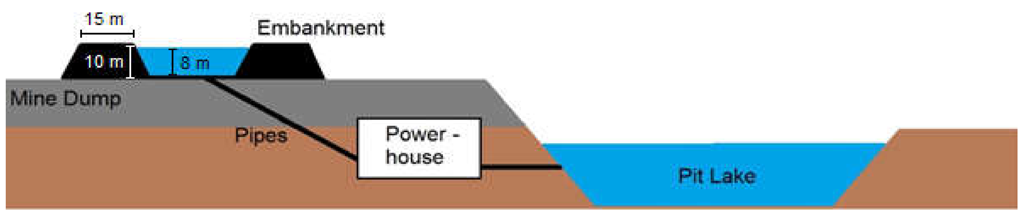
2.5. Technical Concept
2.6. Cost Analysis
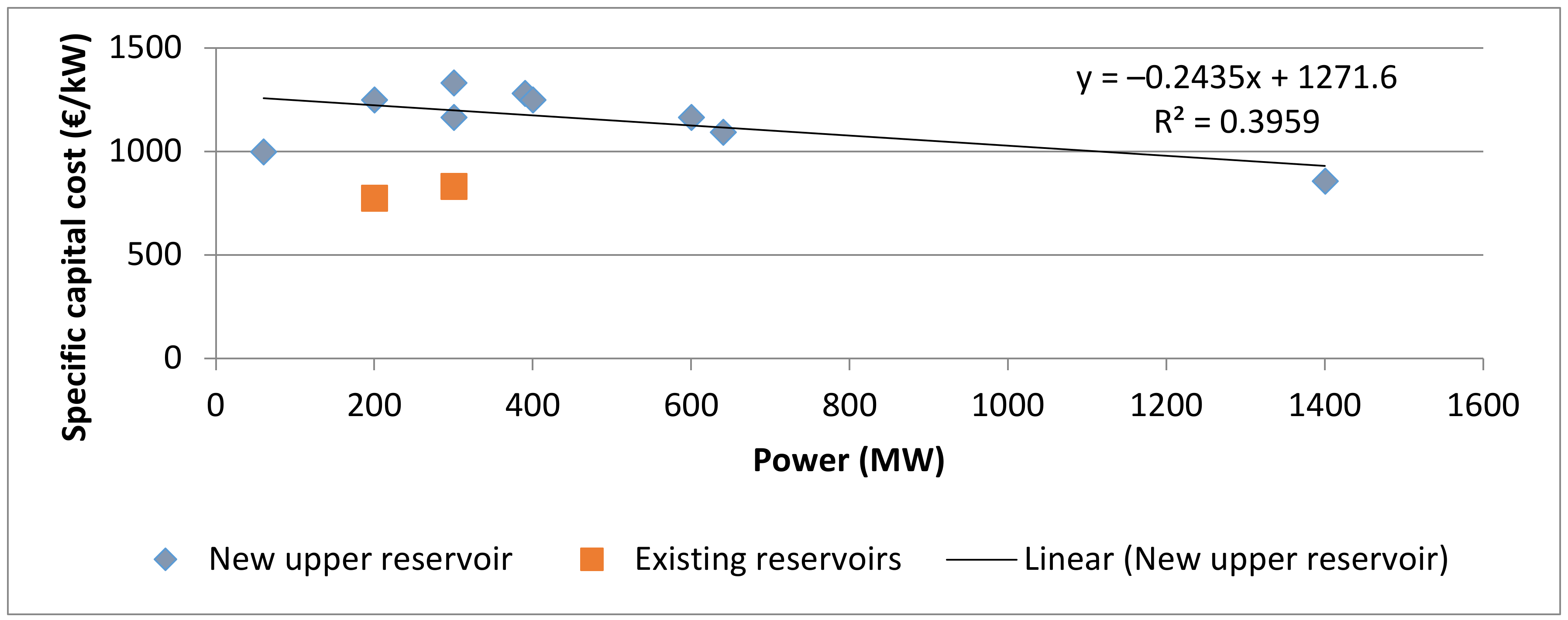
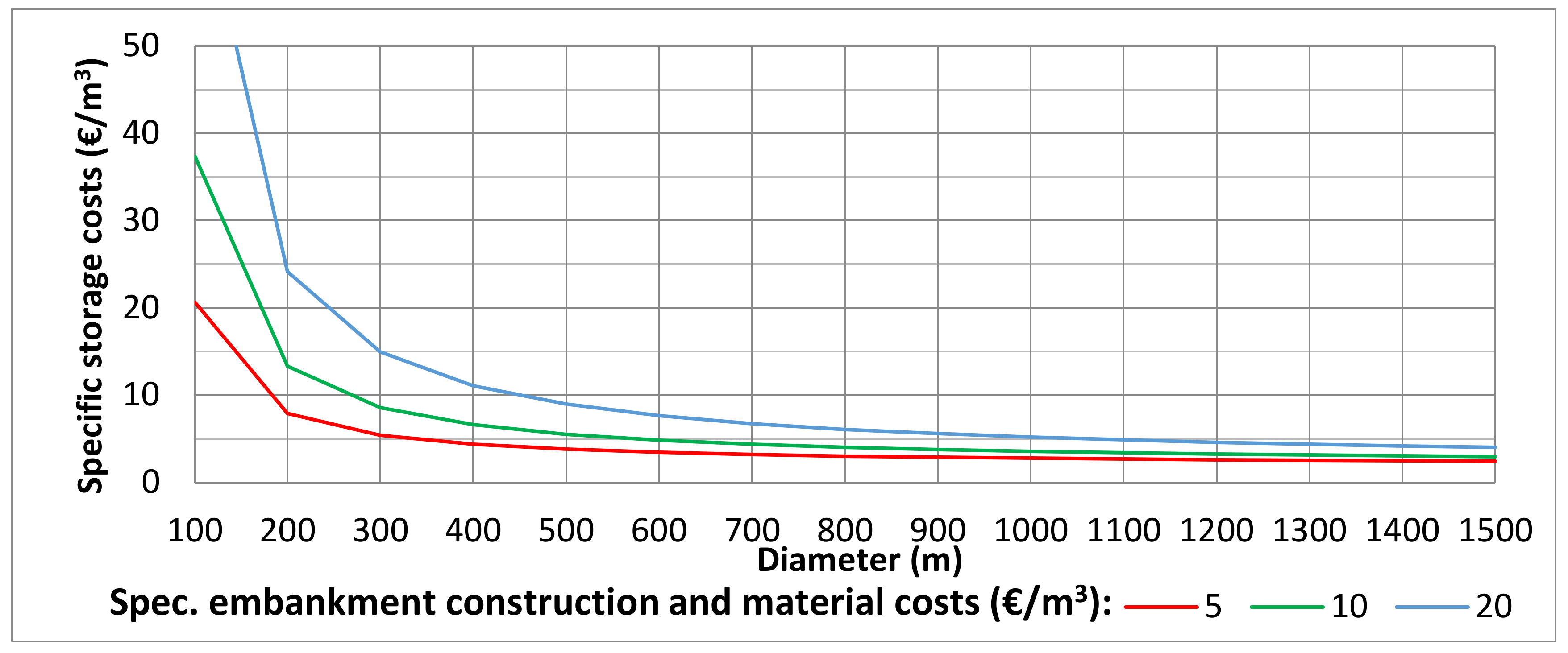
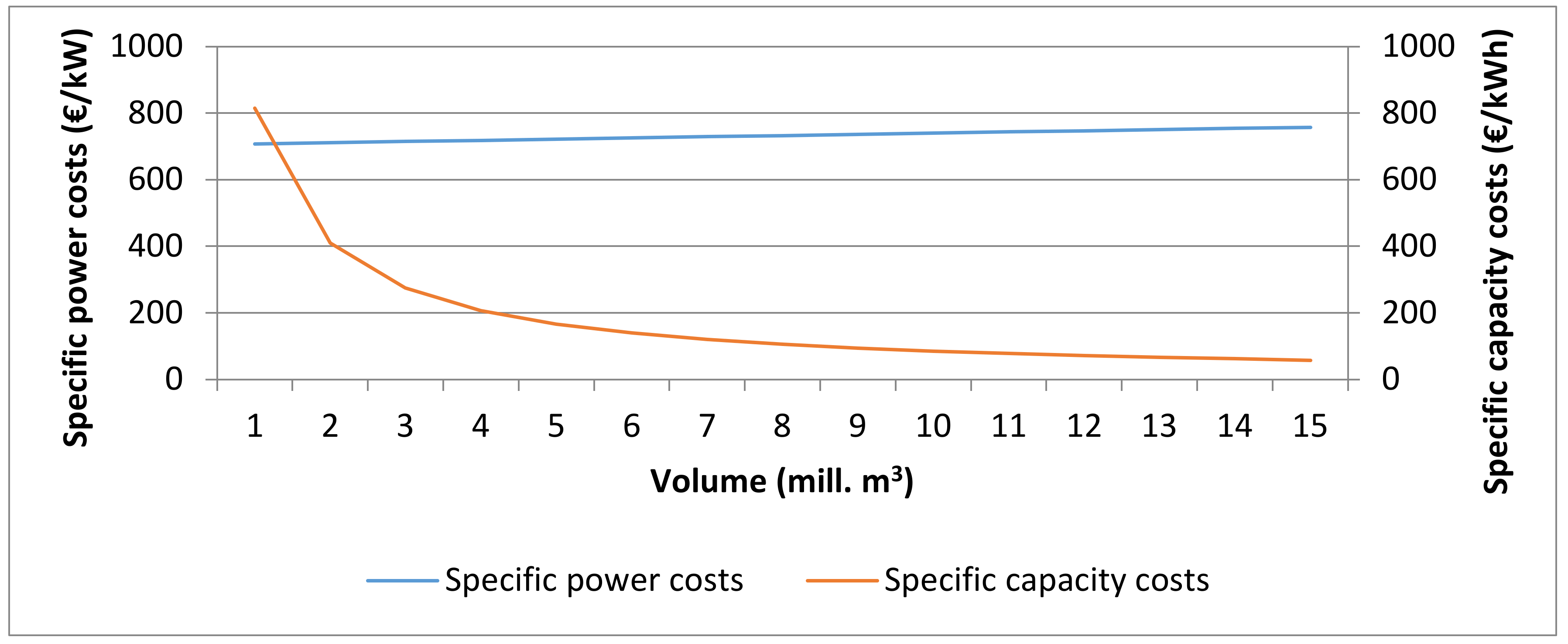
2.6.1. Capital Expenditures (Capex)
2.6.2. Operational Expenditures (Opex)
2.7. Flooding of Pit Lake
2.8. Fees and Regulations
2.8.1. Grid-Use Fees
2.8.2. EEG Levy
2.8.3. Water Extraction Fees
3. Methodology
3.1. Economic Model and Input Description
3.2. Economic Evaluation
3.3. Integration of Cash Flow
3.4. Monte Carlo Simulation
3.4.1. Statistical Testing
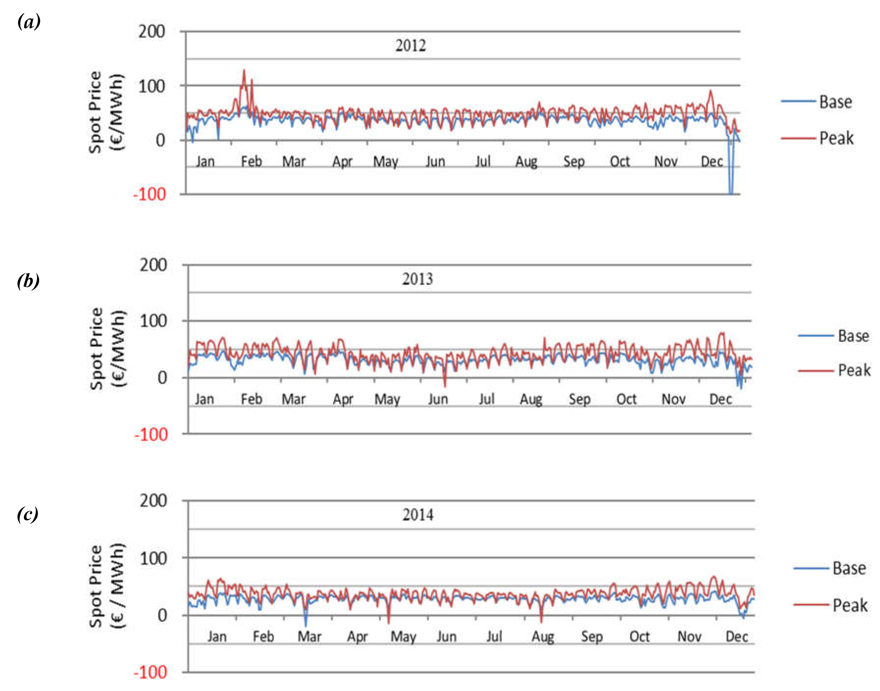
3.4.2. Empirical Analysis of Historical Spot Prices
3.4.3. Simulation of Spot Prices
3.4.4. Retrieval of Secondary Reserve Capacity
3.5. Sensitivity Analysis
4. Results
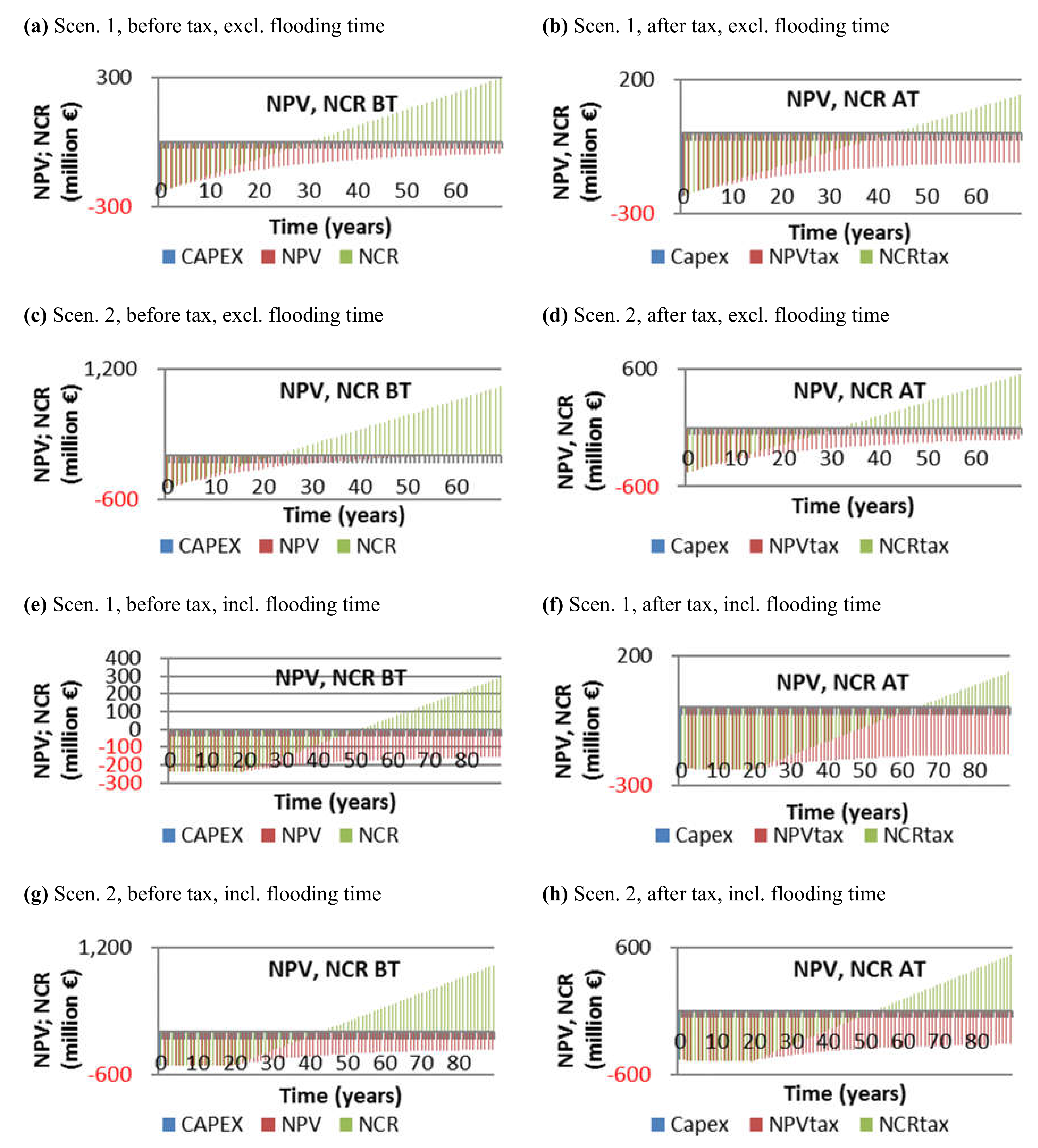
4.1. Economic Evaluation
4.1.1. Excluding Flooding Time
4.1.2. Including Flooding Time
4.2. Sensitivity Analysis
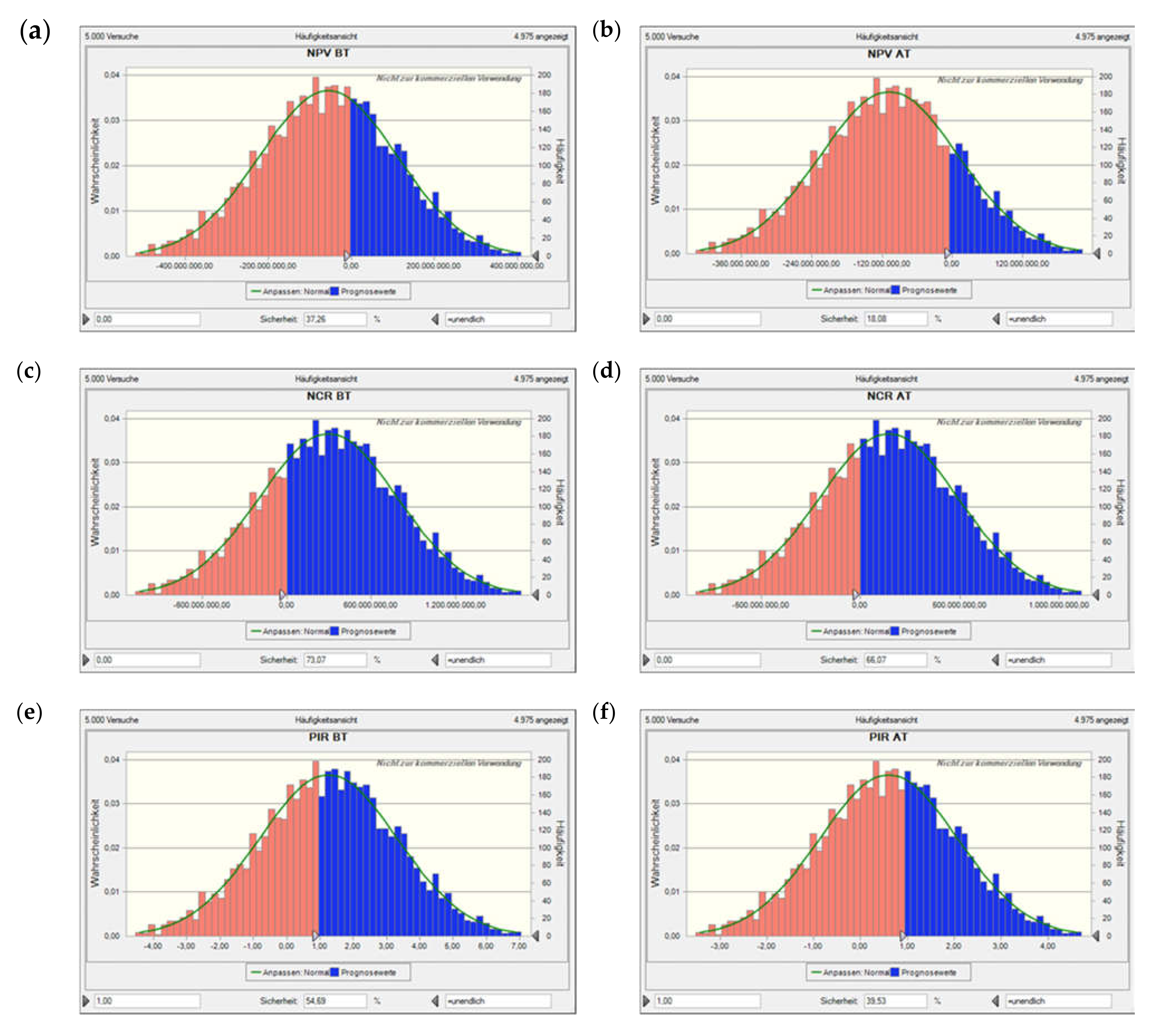
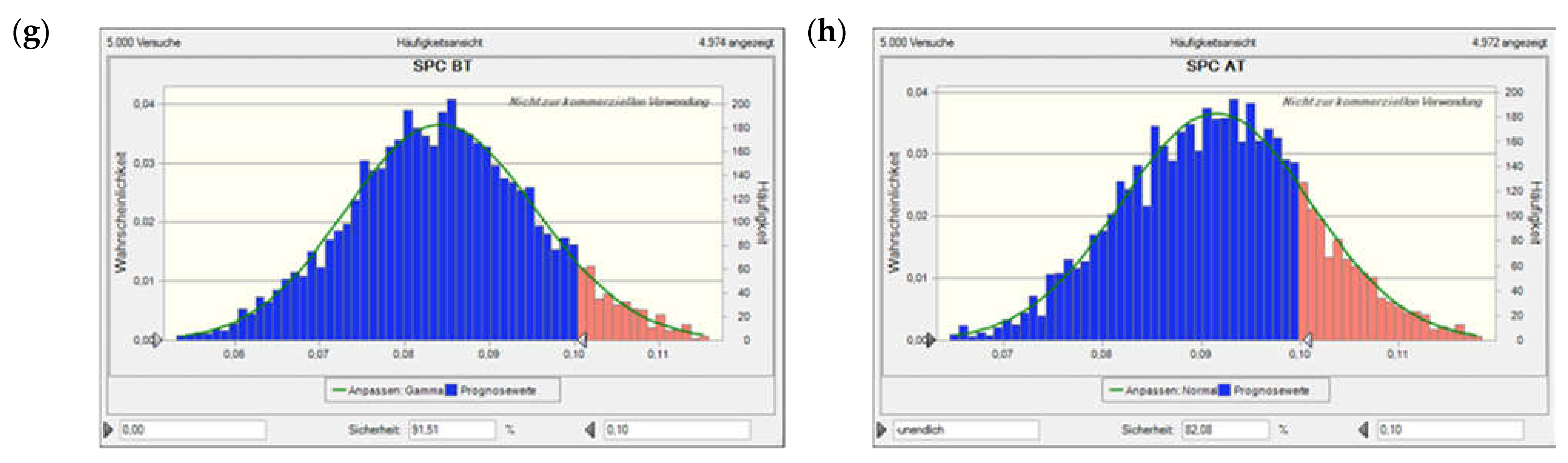
4.3. Value-at-Risk
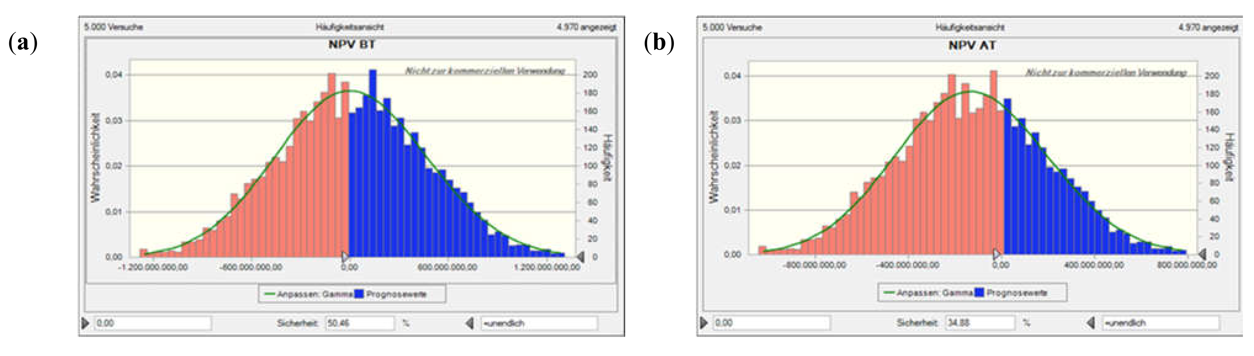
4.3.1. Excluding Flooding Time
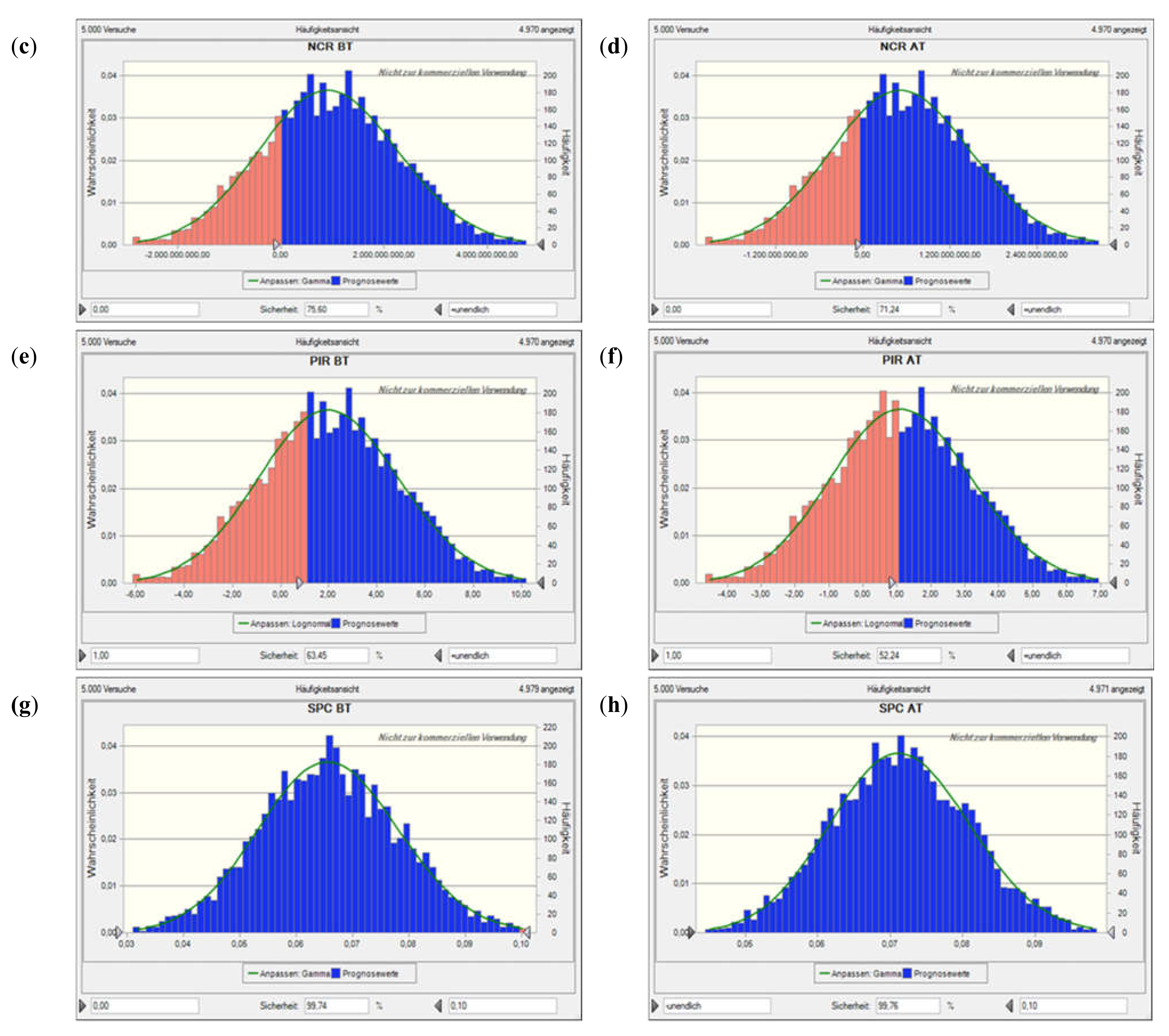
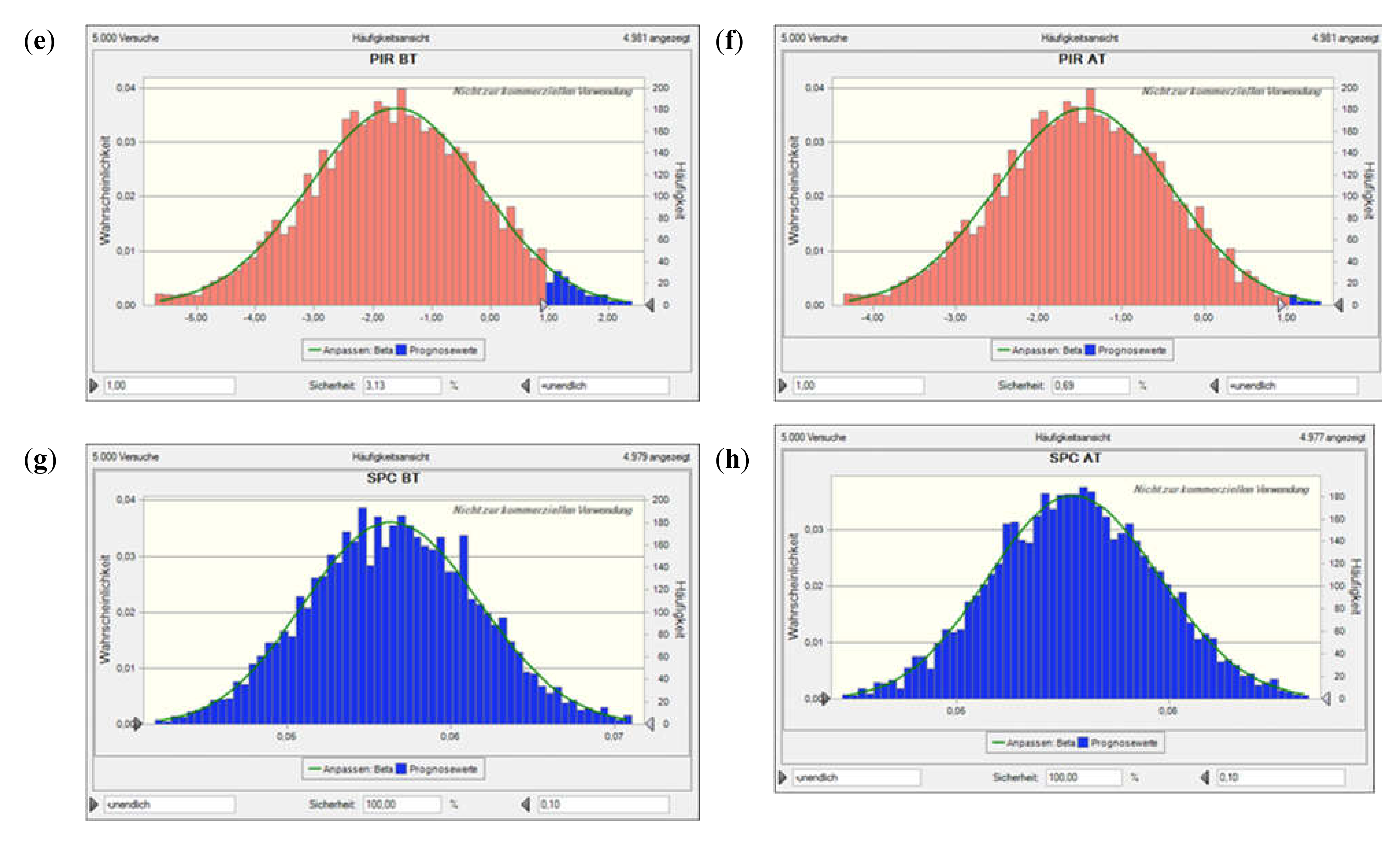
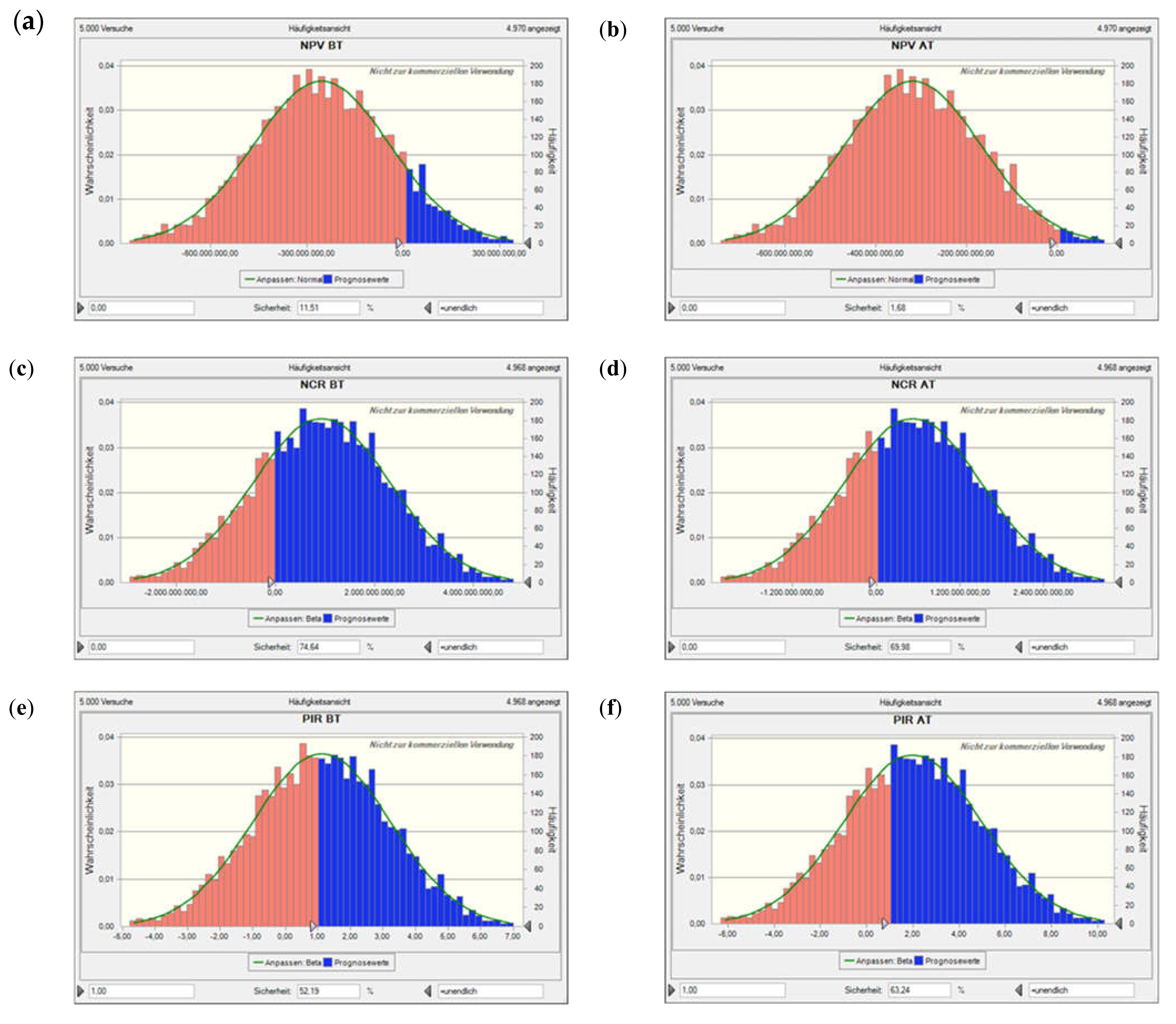
4.3.2. Including Flooding Time
5. Conclusions
Author Contributions
Funding
Acknowledgments
Conflicts of Interest
Abbreviations
| AC | Accruals | LLV | Lake level variation |
| ALR | Area lower reservoir | NC | Network charges |
| AMD | Acid mine drainage | NCR | Net cash recovery |
| AN | Annuity | NPV | Net present value |
| AT | After tax | η | Efficiency |
| ACUR | Area costs upper reservoir | ηd | Efficiency deload |
| AUR | Area upper reservoir | ηl | Efficiency load |
| α | Inclination | om | Operation & maintenance costs |
| BT | Before tax | Opex | Operational expenditures |
| Capex | Capital expenditures | PHS | Pumped hydro storage |
| cd | Capacity deload | PIR | Profit to investment ratio |
| cfix | Opex, fixed | Pl | Power load |
| cl | Capacity load | Pd | Power deload |
| cpower | Spot price per MW bought electricity | ppower | Spot price per MW sold electricity |
| PT | (Dynamic) Payback time | ||
| cvar | Opex, variable | PSR | Electric load for second. reserve market |
| δ | Depreciation rate | ρ | Density of water |
| DRneg | Demand rate secondary reserve, negative base | q | Discounting factor |
| DRpos | Demand rate secondary reserve, positive peak | Qd | Flow rate per turbine deload |
| DUR | Diameter upper reservoir | Ql | Flow rate per turbine load |
| EEG | German Renewable Energy Sources Act (Erneuerbare Energien Gesetz) | r | Inflation |
| EEX | European Energy Exchange | R | Revenues |
| EmbUR | Embankment costs | S | Number of full cycles per year |
| EnWG | German Energy Industry Act (Energiewirtschaftsgesetz) | SealUR | Sealing costs, upper reservoir |
| ERneg | Energy rate secondary reserve, negative base | SPC | Specific production costs |
| ERpos | Energy rate secondary reserve, positive peak | T | Lifetime |
| g | Gravitational constant | T# | Number of machine units |
| h | Height difference | td | Discharge time |
| hd | Full load hours deload per day | tax | Tax rate |
| hl | Full load hours load per day | TSO | Transmission system operator |
| HPFC | Hourly price forward curve | TWh | Terawatt hour |
| HUR | Height upper reservoir | V | Utilizable volume |
| i | Interest rate | vard | Var. costs of deloading per start of unit |
| IPHS | Total Capex | varl | Var. costs of loading per start of unit |
| IPHSp | Capex power-related | varo | Other variable costs |
| IUR | Capex upper reservoir | VLR | Volume lower reservoir |
Appendix A. Spot Market Contracts and Price Data, Water Extraction Fees in Germany

| Contract 1) | Volume of Contract |
|---|---|
| Baseload contract, Block contract for every day, Mon–Sun | 1 MW × 24 h = 24 MWh |
| Peakload contract, Block contract for Mon–Fri, 08:00–20:00 h | 1 MW × 12 h = 12 MWh |
| Weekend baseload contract Block contract Sat 00:00–Sun 24:00 h | 1 MW × 48 h = 48 MWh |
| Hourly contract for every hour of a day | 0.1 MW × 1 h = 0.1 MWh |
| Combination of hourly contracts to hourly blocks | 0.1 MW × number of h |
| EEX – night, 00:00–06:00 h | 0.1 MW × 6 h = 0.6 MWh |
| EEX – morning, 06:00–10:00 h | 0.1 MW × 4 h = 0.4 MWh |
| EEX – business, 08:00–16:00 h | 0.1 MW × 8 h = 0.8 MWh |
| 7 other combinations 2) |
| Federal State | Groundwater | Surface Water | Hydropower |
|---|---|---|---|
| Baden–Wuerttemberg | 5.1 | 1 | 1 |
| Berlin | 31 | - | - |
| Brandenburg | 10 | 2 | 2 |
| Bremen | 2.5 | 0.3 | - |
| Hamburg | 13 | - | - |
| Mecklenburg–Western Pomerania | 5 | 2 | - |
| Lower Saxony | 2.556 | 2.045 | 2.045 |
| North Rhine–Westphalia | 5 | 5 | - |
| Rhineland–Palatinate | 6 | 2.4 | - |
| Saarland | 8 | - | - |
| Saxony | 1.5 | 2 | 0.01 |
| Saxony–Anhalt | 7 | 4 | 4 |
| Schleswig–Holstein | 7 | 0.77 | 0.077 |
| Bavaria | - | - | - |
| Hesse | - | - | - |
| Thuringia | - | - | - |

Appendix B. Statistical Testing
Appendix C. Additional Results


References
- Hohmeyer, O.; Bohm, S. Trends toward 100% renewable electricity supply in Germany and Europe: A paradigm shift in energy policies. Wiley Interdiscip. Rev. Energy Environ. 2015, 4, 74–97. [Google Scholar] [CrossRef]
- Droste-Franke, B. Review of the Need for Storage Capacity Depending on the Share of Renewable Energies. In Electrochemical Energy Storage for Renewable Sources and Grid Balancing; Elsevier: Amsterdam, The Netherlands, 2015; pp. 61–86. [Google Scholar]
- Kapsali, M.; Kaldellis, J. Combining hydro and variable wind power generation by means of pumped-storage under economically viable terms. Appl. Energy 2010, 87, 3475–3485. [Google Scholar] [CrossRef]
- Madlener, R.; Specht, J.M. An Exploratory Economic Analysis of Underground Pumped-Storage Hydro Power Plants in Abandoned Coal Mines. In FCN Working Paper No. 2/2013; Institute for Future Energy Consumer Needs and Behavior, RWTH Aachen University: Aachen, Germany, 2013; (Revised June 2020). [Google Scholar]
- Menéndez, J.; Loredo, J. Use of closured open pit and underground coal mines for energy generation: Application to the Asturias Central Coal Basin (Spain). E3S Web Conf. 2019, 80. [Google Scholar] [CrossRef]
- Menéndez, J.; Loredo, J.; Fernandez, J.M.; Galdo, M. Underground pumped storage hydro power plants with mine water in abandoned coal mines. In Proceedings of the IMWA 2017 (Mine Water and Circular Economy), Lappenranta, Finland, 25–30 June 2017. [Google Scholar]
- Palomino, A.E.C.; Linhares Ferreira, F.C.; Barros, G.P.S.; Silva, L.; Porto, M.P. Conceptual design of a pumped hydro energy storage system for the Aguas Claras open pit mine. In Proceedings of the 23rd ABCM International Congress of Mechanical Engineering, Rio de Janeiro, Brazil, 6–11 December 2015. [Google Scholar]
- Pujades, E.; Orban, P.; Bodeux, S.; Archambeau, P.; Erpicum, S.; Dassargues, A. Underground pumped storage hydropower plants using open pit mines: How do groundwater exchanges influence the efficiency? Appl. Energy 2017, 190, 135–146. [Google Scholar] [CrossRef]
- Pujades, E.; Willems, T.; Bodeux, S.; Orban, P.; Dassargues, A. Underground pumped storage hydroelectricity using abandoned works (deep mines or open pits) and the impact on groundwater flow. Hydrogeol. J. 2016, 24, 1531–1546. [Google Scholar] [CrossRef]
- Northey, S.A.; Mudd, G.M.; Saarivuori, E.; Wessman-Jääskeläinen, H.; Haque, N. Water footprinting and mining: Where are the limitations and opportunities? J. Clean. Prod. 2016, 135, 1098–1116. [Google Scholar] [CrossRef]
- McCullough, C.D.; Marchand, G.; Unseld, J. Mine closure of pit lakes as terminal sinks: Best available practice when options are limited? Mine Water Environ. 2013, 32, 302–313. [Google Scholar] [CrossRef]
- Rehman, S.; Al-Hadhrami, L.; Alam, M. Pumped hydro energy storage system: A technological review. Renew. Sustain. Energy Rev. 2015, 44, 586–598. [Google Scholar] [CrossRef]
- Dena. NNE—Pumpspeicher. Untersuchung der elektrizitätswirtschaftlichen und energiepolitischen Auswirkungen der Erhebung von Netznutzungsentgelten für den Speicherstrombezug von Pumpspeicherwerken. In Final Report Deutsche Energie-Agentur; Deutsche Energie-Agentur: Berlin, Germany, 2008; Available online: https://www.dena.de/fileadmin/dena/Dokumente/Pdf/9112_Pumpspeicherstudie.pdf (accessed on 15 June 2020).
- BVES. Speichertechnologien—Anwendungsbeispiel Pumpspeicherwerk (PSW) Goldisthal. 2016. Available online: https://www.bves.de/wp-content/uploads/2017/04/Pumpspeicherwek.pdf (accessed on 15 June 2020).
- Levron, Y.; Shmilovitz, D. Power systems’ optimal peak-shaving applying secondary storage. Electr. Power Syst. Res. 2012, 89, 80–84. [Google Scholar] [CrossRef]
- Transnet, B.W. Grid Development Plan 2030. 2019. Available online: https://www.netzentwicklungsplan.de/sites/default/files/paragraphs-files/Standard_presentation_GDP_2030_V2019_2nd_draft.pdf (accessed on 15 June 2020).
- IWES. Energiewirtschaftliche Bewertung von Pumpspeicherwerken und anderen Speichern im zukünftigen Stromversorgungssystem. In Final Report Fraunhofer Institut für Windenergie und Energiesystemtechnik (IWES); IWES: Kassel, Germany, 2010; p. 152. [Google Scholar]
- Sensfuß, F.; Ragwitz, M.; Genoese, M. The merit-order effect: A detailed analysis of the price effect of renewable electricity generation on spot market prices in Germany. Energy Policy 2008, 36, 3086–3094. [Google Scholar] [CrossRef]
- Osanloo, M.; Gholamnejad, J.; Karimi, B. Long-term open pit mine production planning: A review of models and algorithms. Int. J. Min. Reclam. Environ. 2008, 22, 3–35. [Google Scholar] [CrossRef]
- Trettin, R.; Glässer, W.; Lerche, I.; Seelig, U.; Treutler, H.-C. Flooding of lignite mines: Isotope variations and processes in a system influenced by saline groundwater. Isot. Environ. Health Stud. 2006, 42, 159–179. [Google Scholar] [CrossRef] [PubMed]
- Höök, M.; Zittel, W.; Schindler, J.; Aleklett, K. Global coal production outlooks based on a logistic model. Fuel 2010, 89, 3546–3558. [Google Scholar] [CrossRef]
- Korbmacher, J. Residual lakes in the Rhineland lignite area. Min. Rep. 2016, 152, 233–244. [Google Scholar]
- Ma, T.; Yang, H.; Lu, L.; Peng, J. Technical feasibility study on a standalone hybrid solar-wind system with pumped hydro storage for a remote island in Hong Kong. Renew. Energy 2014, 69, 7–15. [Google Scholar] [CrossRef]
- Giesecke, J.; Mosonyi, E.; Heimerl, S. Wasserkraftanlagen. Planung, Bau und Betrieb; Springer: Berlin, Germany, 2009. [Google Scholar]
- Popp, M. Nutzung natürlicher Höhenunterschiede; Ingenieurbüro Matthias Popp: Wunsiedel, Germany, 2015; Available online: http://ringwallspeicher.de/Ringwall-Nutzung_naturlicher_Hohenunterschiede.htm (accessed on 15 June 2020).
- Weibel, S.; Madlener, R. Cost-Effective Design of Ringwall Storage Hybrid Power Plants: A Real Options Analysis. Energy Convers. Manag. 2015, 103, 871–885. [Google Scholar] [CrossRef][Green Version]
- RWE. Rahmenbetriebsplan für die Fortführung des Tagebaus Hambach im Zeitraum 2020–2030. 2012. Available online: http://www.rwe.com/web/cms/mediablob/de/1232522/data/60012/2/rwe-power-ag/energietraeger/braunkohle/standorte/tagebau-hambach/Wesentliche-Inhalte.pdf (accessed on 15 June 2020).
- Deane, J.Ó.; Gallachóir, B.; McKeogh, E. Techno-economic review of existing and new pumped hydro energy storage plant. Renew. Sustain. Energy Rev. 2010, 14, 1293–1302. [Google Scholar] [CrossRef]
- Gatzen, C. The Economics of Power Storage: Theory and Empirical Analysis for Central Europe; Oldenburg Industrieverlag: München, Germany, 2008. [Google Scholar]
- B&V Black & Veatch Holding Company. Cost Report. Cost and performance data for power generation technologies. In Report Prepared for the National Renewable Energy Laboratory; National Renewable Energy Laboratory: Golden, CO, USA, 2012; p. 105. Available online: https://refman.energytransitionmodel.com/publications/1921 (accessed on 15 June 2020).
- Steffen, B. Prospects for pumped-hydro storage in Germany. Energy Policy 2012, 45, 420–429. [Google Scholar] [CrossRef]
- Hemm, M.; Nixdorf, B.; Schlundt, A.; Kapfer, M.; Krumbeck, H. Braunkohlentagebauseen in Deutschland. Gegenwärtiger Kenntnisstand über Wasserwirtschaftliche Belange von Braunkohletagebaurestlöchern; With Assistance of Federal Environmental Agency (Umweltbundesamt); Brandenburgische Technische Universität Cottbus: Cottbus, Germany, 2000. [Google Scholar]
- BMJ Federal Office for Justice. Gesetz über die Elektrizitäts- und Gasversorgung. 2005. Available online: https://www.gesetze-im-internet.de/enwg_2005/ (accessed on 15 June 2020).
- BMWiE Federal Ministry for Economic Affairs and Energy. Das Erneuerbare-Energien-Gesetz. 2020. Available online: https://www.erneuerbare-energien.de/EE/Redaktion/DE/Dossier/eeg.html?cms_docId=401818 (accessed on 15 June 2020).
- Netztransparenz.de (2020): EEG-Umlage. Available online: https://www.netztransparenz.de/EEG/EEG-Umlagen-Uebersicht (accessed on 15 June 2020).
- Nebel, A. Energiewirtschaftsrechtliche Einordnung von PSW in Deutschland, Österreich und der Schweiz. In Proceedings of the EFZN Conference, Göttingen, Germany, 21–22 November 2014; pp. 72–91. [Google Scholar]
- European Commission. Directive 2000/60/EC of the European Parliamanet and of the Council of 23 October 2000 on establishing a framework for community action in the field of water policy. Off. J. Eur. Communities 2000, 327, 1–73. [Google Scholar]
- Becker, J.; Mikalauskas, K.; Müller, T. Wasserentnahmeentgelte der Länder—Ein Vergleich. IHK Pfalz Report. 2013. Available online: https://www.ihk-siegen.de/fileadmin/user_upload/Infrastruktur_Planung_und_Verkehr/Broschuere_WEE_Wasserentnahmeentgelte_der_Laender.pdf (accessed on 15 June 2020).
- Bhattacharyya, S.C. Energy Economics; Springer: Berlin, Germany, 2011. [Google Scholar]
- Konstantin, P. Praxisbuch Energiewirtschaft; Springer: Berlin, Germany, 2013. [Google Scholar]
- Zweifel, P.; Praktiknjo, A.; Erdmann, G. Energy Economics. Theory and Applications; Springer: Berlin, Germany, 2017. [Google Scholar]
- Charnes, J. Financial Modeling with Crystal Ball® and Excel; Wiley Sons Inc.: Hoboken, NJ, USA, 2007. [Google Scholar]
- Borchert, J.; Schemm, R.; Korth, S. Stromhandel Institutionen, Marktmodelle, Pricing und Risikomanagement; Schäffer-Poeschel: Stuttgart, Germany, 2006. [Google Scholar]
- Regelleistung.net. Available online: https://www.regelleistung.net/ext/ (accessed on 2 March 2015).
- Greenwood, P.E.; Nikulin, M.S. A Guide to Chi-Squared Testing; John Wiley & Sons, Inc.: Toronto, ON, Canada, 1996. [Google Scholar]
- Hartung, J. Statistik: Lehr- und Handbuch der Angewandten Statistik; Oldenburg Industrieverlag: München, Germany, 2009. [Google Scholar]
- NIST. Anderson-Darling Test. 2020. Available online: https://www.itl.nist.gov/div898/handbook/eda/section3/eda35e.htm (accessed on 15 June 2020).
- RWE RAG. Energiepark Sundern. Available online: http://www.rwe.com/web/cms/mediablob/de/544002/data/0/2/Flyer-Halde-Sundern.pdf (accessed on 15 June 2020).


| Area (km2) | Volume (mill. m3) | Max. Depth (m) | End of Operation | |
|---|---|---|---|---|
| Scen. 1: Hambach | 38 | 5800 | 450 | 2040 |
| Scen. 2: Inden | 11.2 | 800 | 180 | 2030 |
| Country/German Fed. State | Head (m) | Power (MW) | Costs (mill. €) | Planned Completion (a) | Specific Costs (€/kW) | |
|---|---|---|---|---|---|---|
| Vianden M11 | Lux | 280 | 200 | 155 | 2013 | 775 |
| Waldeck 2plus | HE | 360 | 300 | 250 | 2017 | 833.33 |
| Blautal (Ulm) | BW | 170 | 60 | 60 | 2016 | 1000 |
| Schweich (Trier) | RP | 200 | 300 | 400 | 2018 | 1333.33 |
| Forbach | BW | 320-360 | 200 | 250 | 2018 | 1250 |
| Riedl | BY | 350 | 300 | 350 | 2019 | 1166.67 |
| Atdorf | BW | 600 | 1400 | 1200 | 2019 | 857.14 |
| Heimbach | RP | 500 | 600 | 700 | 2019 | 1166.67 |
| Nethe (Höxter) | NW | 220 | 390 | 500 | 2019 | 1282.05 |
| Schmalwasser | TH | 200-300 | 400 | 500 | 2019 | 1250 |
| Simmerath (cancelled) | NW | 240 | 640 | 700 | 2019 | 1093.75 |
| System | Parameter | Symbol | Value | Unit |
|---|---|---|---|---|
| PHS system | Gravity | g | 9.81 | (m/s2) |
| Utilizable volume | V | 10,000,000 | (m3) | |
| Height difference | h | 200 | (m) | |
| Number of turbines | T# | 4 | (-) | |
| Flow rate/Turbine load | Ql | 80 | (m3/s) | |
| Flow rate/Turbine deload | Qd | 100 | (m3/s) | |
| Efficiency load | ηl | 86 | (%) | |
| Efficiency deload | ηd | 88 | (%) | |
| Power load | Pl | 540 | (MW) | |
| Power deload | Pd | 630 | (MW) | |
| Capacity deload | cd | 4360 | (MWh) | |
| Density of water | ρ | 1000 | (kg/m3) | |
| Upper reservoir | Diameter | DUR | 1300 | (m) |
| Height | HUR | 10 | (m) | |
| Freeboard | - | 2 | (m) | |
| Inclination | α | 32 | (°) | |
| Volume | VUR | 10,000,000 | (m3) | |
| Area | AUR | 1.4 × 10⁶ | (m2) | |
| Lower reservoir | Volume | VLR | 5.8 × 10⁹ | (m3) |
| Area | ALR | 40 × 106 | (m2) | |
| Lake level variation | LLV | 0.25 | (m) |
| Parameter | Symbol | Value | Unit |
|---|---|---|---|
| Capex, power-related | IPHSp | 704 | (€/MW) |
| Capex, upper reservoir | IUR | 16 × 106 | (€) |
| Area costs | ACUR | 5 | (€/m2) |
| Embankment costs | EmbUR | 5 | (€/m3) |
| Sealing costs | SealUR | 10 | (€/m2) |
| Opex, fixed | cfix | - | (€/a) |
| Operation and maintenance | Om | 10,000 | (€/Mwa) |
| Opex, variable | cvar | - | (€/a) |
| Start loading | varl | 2 | (€/MW/start) |
| Start deloading | vard | 2 | (€/MW/start) |
| Other | varo | 1 | (€/MWh) |
| Parameter | Symbol | Value | Unit |
|---|---|---|---|
| Power market | - | - | (-) |
| Full cycles per year | S | 350 | (-) |
| Spot price per MW sold electricity | ppower | 43 | (€/MWh) |
| Spot price per MW bought electricity | cpower | 24 | (€/MWh) |
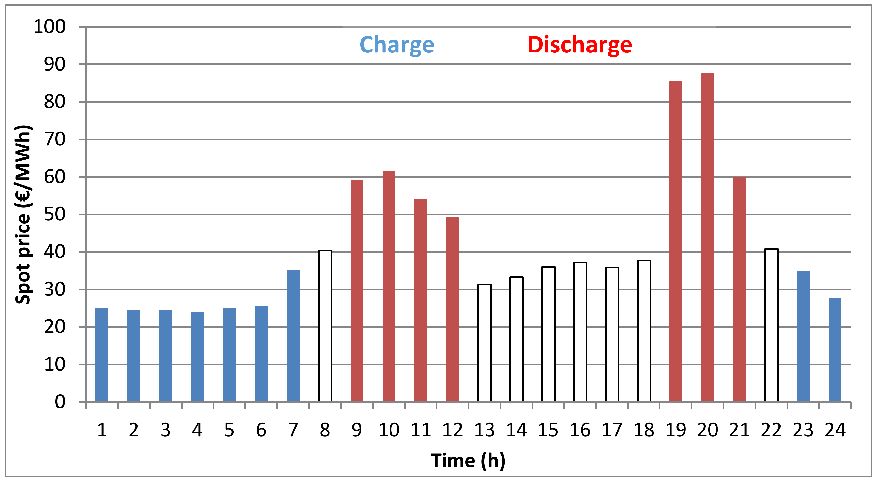
| Full-load hours load | hl | 9 | (h) |
| Full-load hours deload | hd | 7 | (h) |
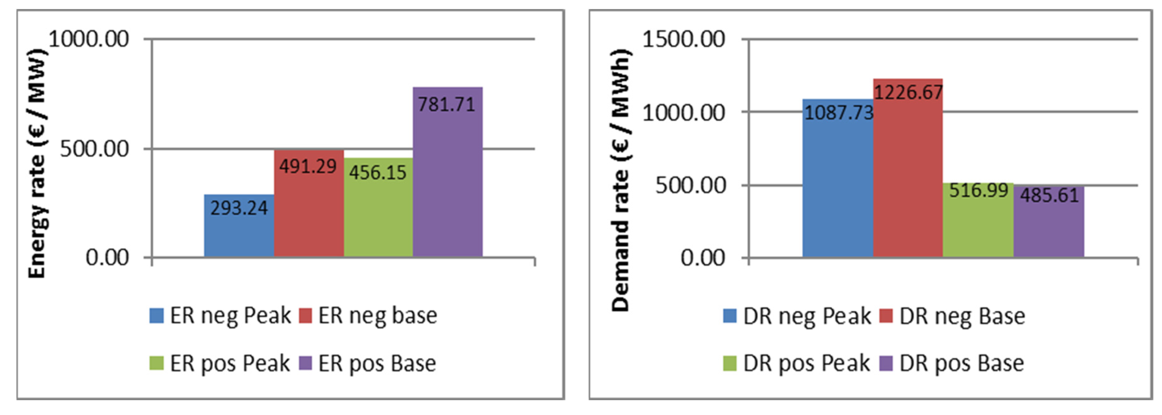
| Demand rate sec. res. market pos. peak | ERpos | 517 | (€/MWh/w) |
| Energy rate sec. res. market pos. peak | DRpos | 456 | (€/MW/w) |
| Demand rate sec. res. market neg. base | ERneg | 1227 | (€/MWh/w) |
| Energy rate sec. res. market neg. base | DRneg | 491 | (€/MW/w) |
| Electricity load for sec. res. market | PSR | 20 | (MW) |
| Parameter | Symbol | Value | Unit |
|---|---|---|---|
| Depreciation rate | δ | 10 | (%) |
| Accruals | AC | 10 | (%) |
| Interest rate | i | 6 | (%) |
| Inflation rate | r | 2 | (%) |
| Tax rate | tax | 29 | (%) |
| Discounting factor (nominal) | q | 1.06 | (-) |
| Lifetime | T | 70 | (a) |
| Variable | Symbol | Unit |
|---|---|---|
| Revenues | R | (€) |
| Capex | IPHS | (€) |
| Opex, fixed | cfix | (€) |
| Opex, variable | cvar | (€/MWh) |
| Specific production costs | SPC | (€/MW) |
| Annuity | AN | (€/MW) |
| Net cash recovery | NCR | (€) |
| Net present value | NPV | (€) |
| Profit to investment ratio | PIR | (-) |
| Payback time | PT | (a) |
| Distribution | Anderson–Darling | Kolmogorov–Smirnov | Chi-Square |
|---|---|---|---|
| Logistical | 7.0802 | 0.0340 | 392.2842 |
| Student t | 7.6012 | 0.0372 | 422.8631 |
| Normal | 19.7925 | 0.0594 | 427.6037 |
| Beta | 20.3815 | 0.0601 | 445.2282 |
| Gamma | 21.7549 | 0.0635 | 470.0104 |
| Lognormal | 25.0144 | 0.0689 | 463.6037 |
| Weibull | 105.8409 | 0.0971 | 1210.7093 |
| Min. extreme value | 106.4567 | 0.0974 | 1218.9935 |
| Max. extreme value | 348.3581 | 0.1848 | 2505.8175 |
| Beta PERT | 586.6824 | 0.2649 | 4767.9974 |
| Triangular | 945.5238 | 0.3793 | 5482.0130 |
| Uniform | 1545.4198 | 0.4844 | 13,001.1786 |
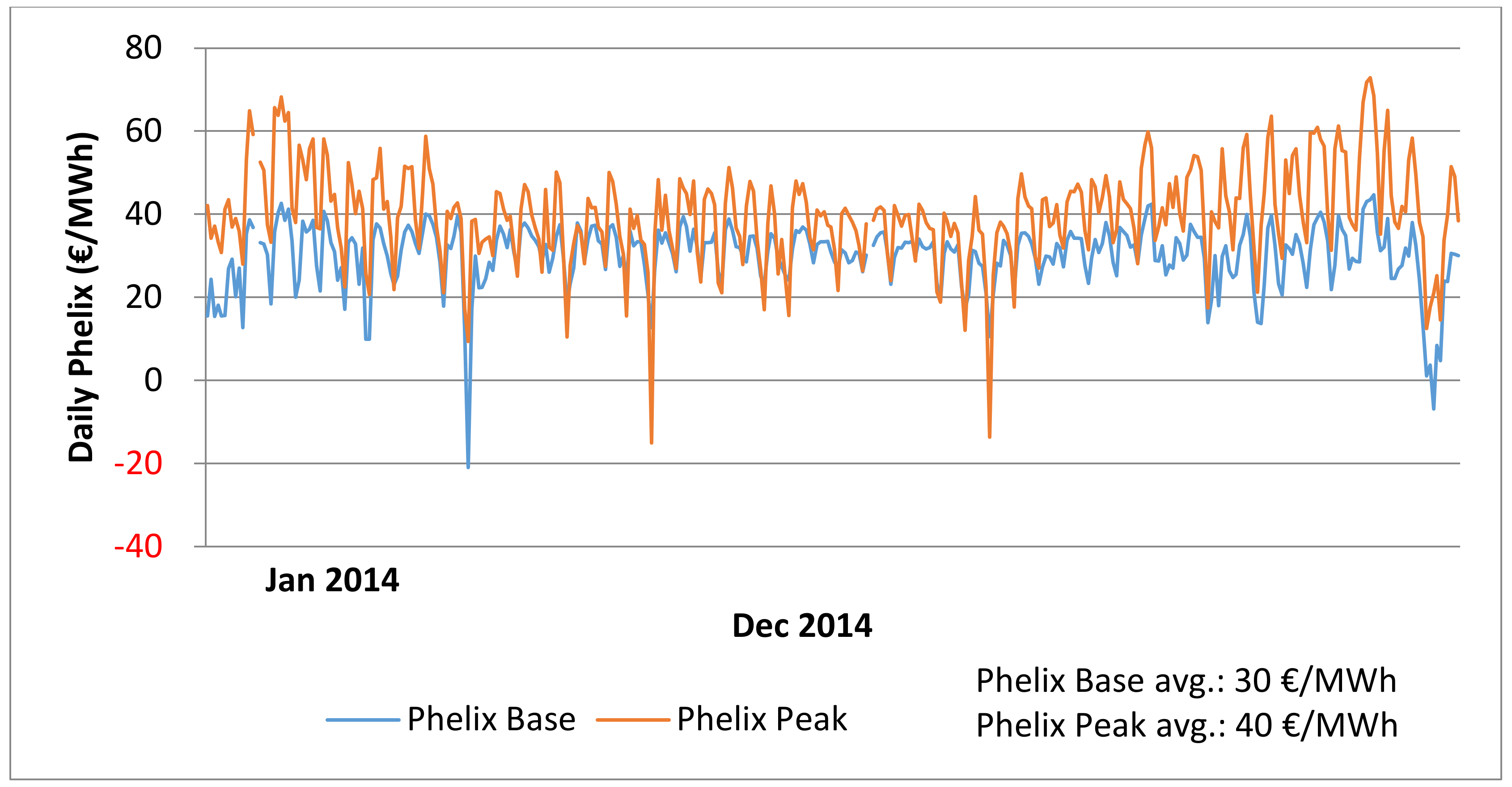
| Year | Base (9 p.m.–8 a.m.) | Peak (8 a.m.–9 p.m.) | Price Spread | ||
|---|---|---|---|---|---|
| Mean (€/MWh) | Std. Dev. (€/MWh) | Mean (€/MWh) | Std. Dev. (€/MWh) | Mean (€/MWh) | |
| 2009 | 29.60 | 12.00 | 46.68 | 13.66 | 17.08 |
| 2010 | 36.98 | 7.59 | 50.83 | 10.52 | 13.85 |
| 2011 | 43.88 | 8.29 | 57.26 | 9.34 | 13.38 |
| 2012 | 35.38 | 14.98 | 48.70 | 13.83 | 13.32 |
| 2013 | 31.12 | 9.16 | 43.38 | 14.48 | 12.26 |
| 2014 | 27.89 | 10.45 | 37.41 | 12.90 | 9.52 |
| Pos. SBC | Offered Capacity (MW) | Demand Rate (€/MWh) | Energy Rate (€/MW) | |||
|---|---|---|---|---|---|---|
| Peak | Base | Peak | Base | Peak | Base | |
| Mean | 32.88 | 24.27 | 516.99 | 485.61 | 456.15 | 781.71 |
| Std. Dev. | 16.48 | 16.81 | 961.79 | 902.27 | 52.67 | 84.36 |
| Max. | 67.71 | 75.48 | 5160.12 | 4864.63 | 589.35 | 988.36 |
| Min. | 5.00 | 5.00 | 57.72 | 56.48 | 352.63 | 608.78 |
| Neg. SBC | Offered Capacity (MW) | Demand Rate (€/MWh) | Energy Rate (€/MW) | |||
| Peak | Base | Peak | Base | Peak | Base | |
| Mean | 19.73 | 21.46 | 1087.73 | 1226.67 | 293.24 | 491.29 |
| Std. Dev. | 15.47 | 16.12 | 1882.51 | 1972.79 | 73.10 | 80.94 |
| Max. | 75.75 | 67.48 | 6006.76 | 5982.51 | 538.33 | 659.44 |
| Min. | 5.00 | 5.00 | 0.31 | 0.89 | 163.64 | 316.51 |
| Scenario Parameter | Unit | Scen. 1 (Inden) | Scen. 2 (Hambach) |
|---|---|---|---|
| Head | (m) | 100 | 200 |
| Storage volume | (m3) | 6,000,000 | 10,000,000 |
| Pit lake volume | (m3) | 800,000,000 | 5,800,000,000 |
| Lake level variation | (m/d) | 0.54 | 0.25 |
| Duration of flooding * | (a) | 20 | 22 |
| Power | (MW) | 314 | 628 |
| Capacity | (MWh) | 1308 | 4360 |
| Yearly production | (MWh) | 457,800 | 1,526,000 |
| Cash Flow Items: | |||
| Investment | |||
| PHS system | (1000 €) | 221,000 | 442,000 |
| Storage | (1000 €) | 15,000 | 25,000 |
| Annual Revenues | |||
| Peak shaving | (1000 €) | 21,517 | 66,264 |
| Pos SBC | (1000 €) | 1750 | 1750 |
| Neg SBC | (1000 €) | 1787 | 1787 |
| Annual Operating Costs | |||
| Fixed | (1000 €) | 3139 | 6278 |
| Variable | (1000 €) | 13,940 | 43,198 |
| Annual accruals | (1000 €) | 425 | 833 |
| NCR BT | (1000 €) | 296,949 | 955,664 |
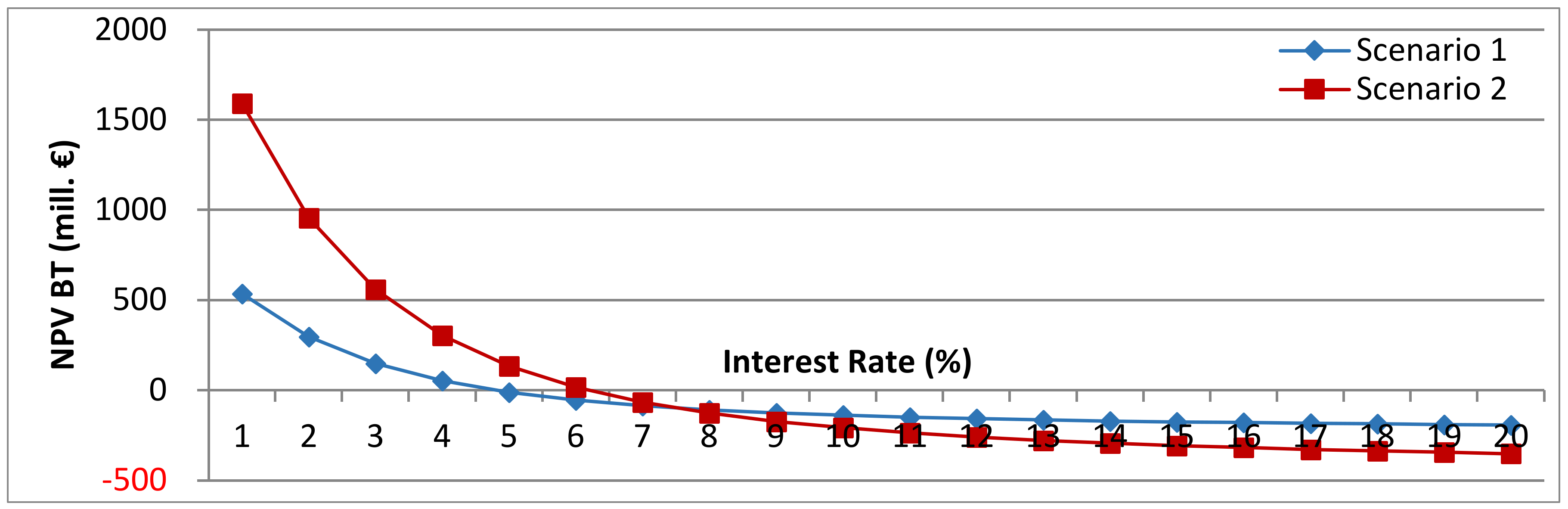
| NPV BT | (1000 €) | −54,998 | 16,170 |
| PIR BT | (-) | 1.26 | 2.05 |
| SPC BT | (€/kWh) | 0.08 | 0.07 |
| PT BT | (a) | n.a. | n.a. |
| Annual depreciation | (1000 €) | 3371 | 6671 |
| Annual tax | (1000 €) | 2208 | 5894 |
| NCR AT | (1000 €) | 142,394 | 543,091 |
| NPV AT | (1000 €) | −107,489 | −123,950 |
| PIR AT | (-) | 0.60 | 1.16 |
| SPC AT | (€/kWh) | 0.09 | 0.07 |
| PT AT | (a) | n.a. | n.a. |
| Cash Flow Item | Unit | Scen. 1 (Inden) | Scen. 2 (Hambach) |
|---|---|---|---|
| NCR BT | (1000 €) | 290,670 | 943,106 |
| NPV BT | (1000 €) | −156,433 | −251,727 |
| PIR BT | (-) | 1.23 | 2.02 |
| PT BT | (a) | n.a. | n.a. |
| NCR AT | (1000 €) | 136,115 | 530,534 |
| NPV AT | (1000 €) | −180,753 | −316,648 |
| PIR AT | (-) | 0.6 | 1.14 |
| PT AT | (a) | n.a. | n.a. |
| Distribution | Mean | Std. Dev. | Conf. Level (%) | ||
|---|---|---|---|---|---|
| (a) Scen. 1 | |||||
| NPV (mill. €) | BT | normal | −55.59 | 165.55 | >0; 37.26 |
| AT | normal | −107.91 | 117.54 | >0; 18.8 | |
| NCR (mill. €) | BT | normal | 295.22 | 165.55 | >0; 73.07 |
| AT | normal | 141.16 | 346.01 | >0; 66.07 | |
| PIR (-) | BT | normal | 1.25 | 2.07 | >1; 54.69 |
| AT | normal | 0.6 | 1.47 | >1; 39.53 | |
| SPC (€/kWh) | BT | gamma | 0.08 | 0.01 | <0.1; 91.51 |
| AT | normal | 0.09 | 0.01 | <0.1; 39.53 | |
| (b) Scen. 2 | |||||
| NPV (mill. €) | BT | gamma | 14.04 | 461.37 | >0; 50.46 |
| AT | gamma | −125.46 | 327.58 | >0; 34.88 | |
| NCR (mill. €) | BT | gamma | 949.4 | 1358.48 | >0; 75.6 |
| AT | gamma | 538.64 | 964.53 | >0; 71.24 | |
| PIR (-) | BT | lognormal | 2.03 | 2.91 | >1; 63.45 |
| AT | lognormal | 1.15 | 2.07 | >1; 52.24 | |
| SPC (€/kWh) | BT | lognormal | 0.07 | 0.01 | <0.1; 99.74 |
| AT | gamma | 0.07 | 0.01 | <0.1; 99.76 |
| Variable (unit) | Distribution | Mean | Std. Dev. | Conf. Level (%) | |
|---|---|---|---|---|---|
| Scen. 1 | |||||
| NPV (mill. €) | BT | Beta | −263.57 | 53.66 | >0; 0.0 |
| AT | Beta | −256.82 | 38.10 | >0; 0.0 | |
| NCR (mill. €) | BT | Beta | −390.18 | 341.03 | >0; 12.75 |
| AT | Beta | −347.23 | 242.13 | >0; 7.38 | |
| PIR (-) | BT | Beta | −1.65 | 1.45 | >1; 3.13 |
| AT | Beta | −1.47 | 1.03 | >1; 0.69 | |
| SPC (€/kWh) | BT | Beta | 0.06 | 0.01 | <0.1; 100 |
| AT | Beta | 0.06 | 0.0 | <0.1; 100 | |
| Scen. 2 | |||||
| NPV (mill. €) | BT | Normal | −254.77 | 212.54 | >0; 11.51 |
| AT | Normal | −318.81 | 150.91 | >0; 1.68 | |
| NCR (mill. €) | BT | Beta | 930.15 | 1380.99 | >0; 74.64 |
| AT | Beta | 521.33 | 980.50 | >0; 69.98 | |
| PIR (-) | BT | Beta | 1.99 | 2.96 | >1; 52.19 |
| AT | Beta | 1.14 | 2.1 | >1; 63.24 | |
| SPC (€/kWh) | BT | Beta | 0.04 | 0.01 | <0.1; 100 |
| AT | Normal | 0.04 | 0.00 | <0.1; 100 | |
© 2020 by the authors. Licensee MDPI, Basel, Switzerland. This article is an open access article distributed under the terms and conditions of the Creative Commons Attribution (CC BY) license (http://creativecommons.org/licenses/by/4.0/).
Share and Cite
Wessel, M.; Madlener, R.; Hilgers, C. Economic Feasibility of Semi-Underground Pumped Storage Hydropower Plants in Open-Pit Mines. Energies 2020, 13, 4178. https://doi.org/10.3390/en13164178
Wessel M, Madlener R, Hilgers C. Economic Feasibility of Semi-Underground Pumped Storage Hydropower Plants in Open-Pit Mines. Energies. 2020; 13(16):4178. https://doi.org/10.3390/en13164178
Chicago/Turabian StyleWessel, Michael, Reinhard Madlener, and Christoph Hilgers. 2020. "Economic Feasibility of Semi-Underground Pumped Storage Hydropower Plants in Open-Pit Mines" Energies 13, no. 16: 4178. https://doi.org/10.3390/en13164178
APA StyleWessel, M., Madlener, R., & Hilgers, C. (2020). Economic Feasibility of Semi-Underground Pumped Storage Hydropower Plants in Open-Pit Mines. Energies, 13(16), 4178. https://doi.org/10.3390/en13164178