Electrical Damping Assessment and Sensitivity Analysis of a Liquefied Natural Gas Plant: Experimental Validation

Abstract

Liquefied Natural Gas (LNG) plants are commonly island-operated weak grids where the interaction of high-power Variable Frequency Drives (VFDs) with the Turbine-Generator (TG) units might cause Sub-Synchronous Torsional Interaction (SSTI) phenomena. SSTI phenomena can lead the LNG plant to instability conditions. Each LNG plant configuration is characterized by a risk level, which is considered high when the electrical damping at the TG Torsional Natural Frequencies (TNFs) is negative. Starting from a real case study, a detailed electromechanical model of an LNG plant is presented. The model is comprehensive of the control system of the power conversion stage and of the TG unit. Sensitivity analysis, performed on control system parameters, allows one to detect the parameters that impact the electrical damping and the stability of the overall LNG plant. A complete simulation platform is developed. Experimental results are carried out on a real LNG plant considering four different configurations. The theoretical model and the simulation platform allow one to estimate the electrical damping and the results are confirmed by the experimental validation. It is demonstrated that fine tuning of the power conversion stage control parameters can reduce the risk related to torsional instability.

1. Introduction

Up-to-date Liquefied Natural Gas (LNG) plants are highly electrified and based on high power electrical motors supplied by Variable Frequency Drives (VFDs). The interaction among the VFDs and the Turbine-Generator (TG) units may cause torsional vibrations known as Sub-Synchronous Torsional Interactions (SSTIs) [1,2,3]. Over the last years some SSTI phenomena have been experienced on site in the LNG plants by the authors. One of the most significant occurred during the commissioning phase and the event is used as a case study for the present paper.

When SSTI phenomena occur, the torsional vibrations measured on the TG shaft-line generate electric disturbances such as voltage fluctuations in the power system. The voltage fluctuations in input to the VFDs imply current fluctuations at the VFD DC link and at the VFD output. Finally, high torsional vibrations can lead to torsional instability.

In the literature the first studies focused on the torsional instability risk assessment are related to the Sub Synchronous Resonance (SSR) phenomenon [4,5,6,7]. In [4], the generator damping, measured at no load condition, is used as an index value to define the risk. In [5] the compensation impact factor is used to detect SSR risks in the case of series compensated transmission lines. In [6] the impact of the transmission expansion on the system damping is evaluated using the frequency-scan approach. In [7] the SSR risk is detected comparing the electrical damping with the modal damping.

The most used risk assessment technique is based on the Unit Interaction Factor (UIF) calculation, originally introduced for HVDC applications [8]. For oil and gas applications, the method implies high variations of the threshold value adopted to evaluate the risk, for this reason the UIF technique is not always feasible.

In this paper, the risk assessment for an LNG plant is based on the electrical damping evaluation. The torsional instability risk can be considered high when the electrical damping at the Torsional Natural Frequencies (TNFs) is negative. Hence the risk assessment relies on the electrical damping assessment.

In [1] a connection between the power electronics analysis and the power systems analysis is established and a complete model of a LNG plant is provided combining the dynamic model of the power conversion stage and the TG electromechanical model. The sole theoretical model allows electrical damping assessment in the case of a basic LNG plant configuration with one TG unit and one VFD. However the analysis provided in [1] lacks a deep investigation about the impact of the synchronization system design on the electrical damping estimation. In the same model the design of the TG controller is not considered.

Some previous studies such as [9,10] have shown that the synchronization system parameters affect the power system stability in the case of weak grids. Besides the impact of the Power System Stabilizer (PSS) on the SSR damping has been previously demonstrated in [11,12,13,14]. Aware of these considerations and starting from the combined electromechanical model developed in [1], the same authors present in this paper a more accurate model providing the electrical damping assessment. Differently from the model presented in [1], both the control systems of the VFD and of the TG unit are included in the overall model. It allows one to detect which control parameters have more impact on the generator units’ electrical damping. Moreover a classical tool such as the sensitivity analysis [15,16,17] is adopted for this purpose. In particular the Finite Difference Method (FDM) [18] is employed to achieve a local sensitivity study. The overall advanced model is the first original contribution of the paper compared to [1].

Nevertheless, it has to pointed out that in the case of complex LNG plant configurations, with numerous TG units and several VFDs, the calculation of the electrical damping by the theoretical model can exhibit some practical limitations. Starting from this consideration, a complete simulation platform, which emulates the theoretical model, is developed and the results are shown in the paper. The complete simulation platform allows one to analyze also the complex LNG plant configurations and to extend the results of this study to different plants. The flexibility relies in the possibility to adapt the software to different power ranges and a different kind of loads, including also changes of the operational TG units’ number in real time. Finally, an extensive test campaign has been carried out on a real LNG plant in order to take into account also commissioning and potential grid contingencies. These products represent innovative contributions compared to [1].

In conclusion, the theoretical outcomes are confirmed by the simulation and experimental results. The electrical damping assessment allows one to determine the risk of the LNG plant considering different configurations. It is also demonstrated that the proper tuning of the control parameters can modify the electrical damping and, as a consequence, can influence the LNG plant level of risk.

The rest of the paper is organized as follows: in Section 2 the LNG plant configuration is presented; in Section 3 and in Section 4 there are proposed, respectively, the detailed TG unit and VFD models and a preliminary sensitivity analysis is performed; Section 5 treats the LNG plant simulation platform; in Section 6 the simulation and experimental results are shown; in Section 7 a brief discussion about the future insights and possible applications is presented; finally Section 8 is focused on final remarks.

2. LNG Plant Configuration

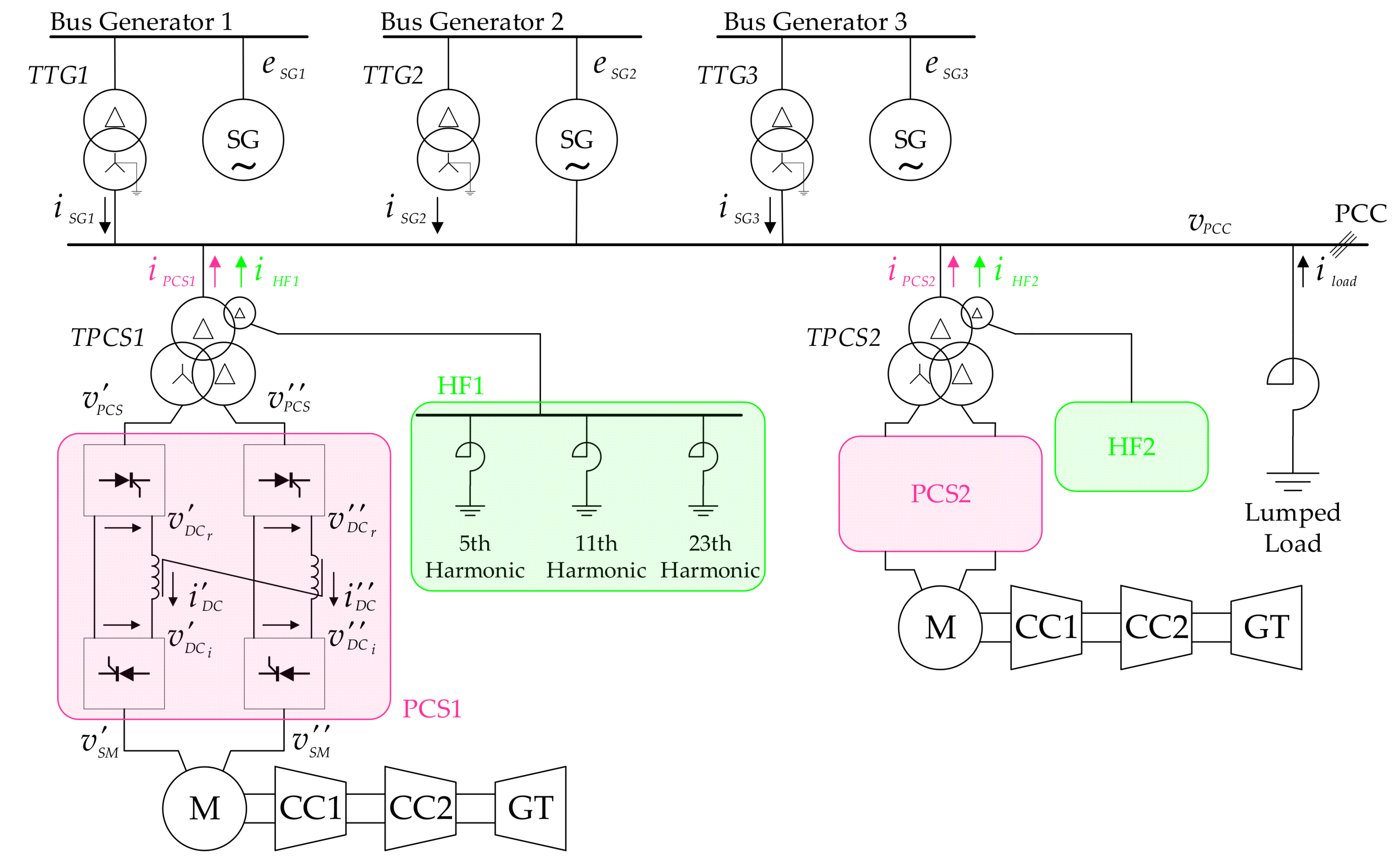
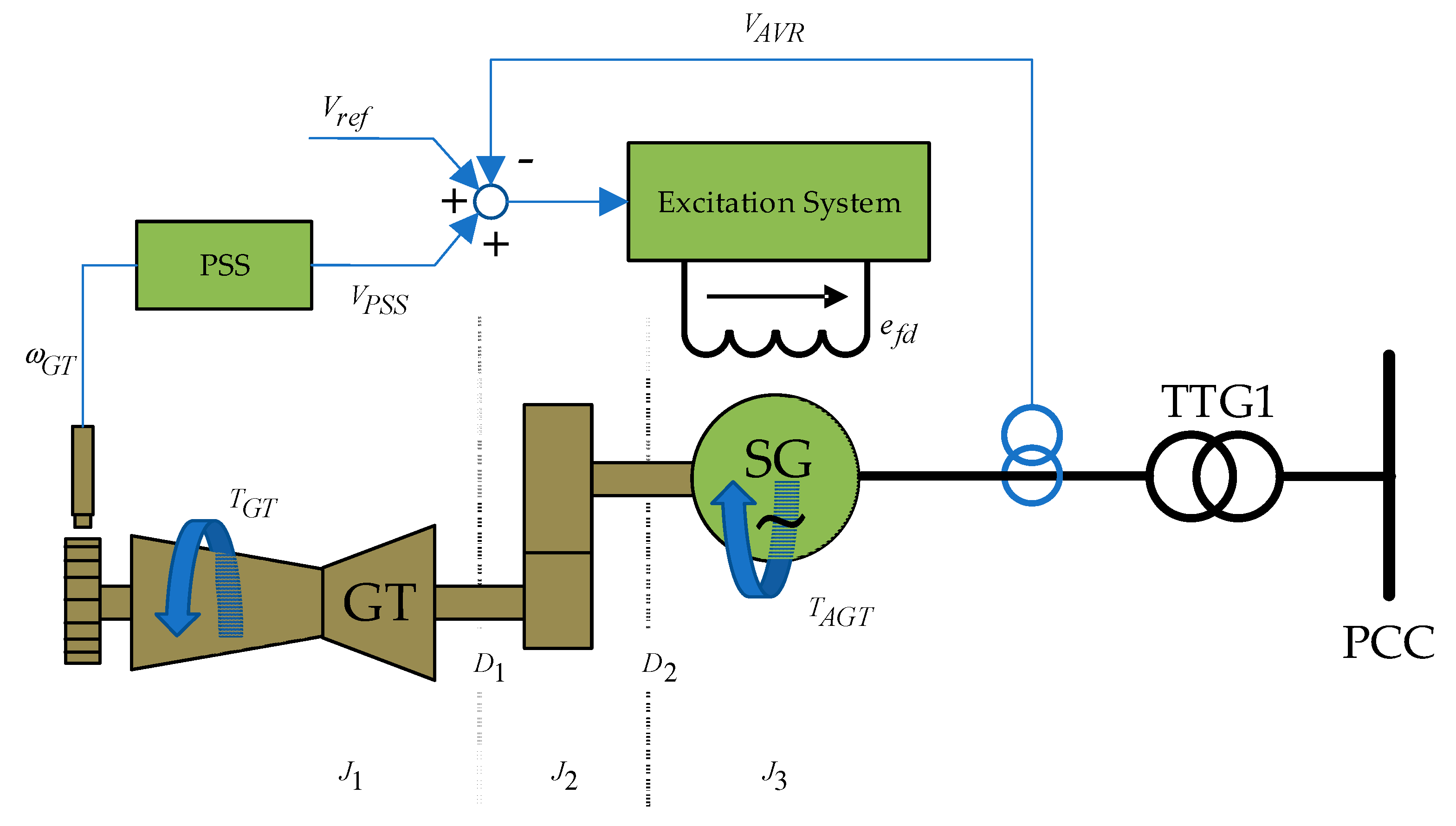
The LNG plant under analysis is shown in Figure 1. The considered power system is composed of three identical Gas Turbines (GTs) connected to three identical Synchronous Generators (SGs). For the sake of simplicity, Figure 1 represents only the SGs while the complete TG unit is depicted in Figure 2. The SGs are connected to the Point of Common Coupling (PCC) through three step-up transformers, denoted as TTG1, TTG2 and TTG3. Two compression trains operate the natural gas liquefaction. Each compression train is composed of two centrifugal compressors (CC1 and CC2), a GT (the prime mover) and a synchronous Motor (M). M acts as starter and helper motor, which allows one to start-up the entire train and provides additional power when required. The motors are supplied by two power conversion stages denoted as PCS1 and PCS2. The power conversion stages are two Thyristor Variable frequency Drives (TVFDs). Each TVFD is connected to the PCC through a step-down transformer with two secondary windings. The two step-down transformers are indicated with TPCS1 and TPCS2 and adapt the voltage level in order to supply the TVFDs. Each TVFD consists of two Line-Commutated-Converters (LCCs). Each LCC is a double-stage converter since the first stage is a line-commutated-rectifier (LCR), while the second stage is a Line-Commutated-Inverter (LCI). The fundamental frequency of the LCRs is the grid frequency f_n. The LCIs supply the synchronous motor M, hence the LCIs fundamental frequency is the motor frequency denoted as f_m. Each TVFD is based on 6-pulse H-Bridges.

A Harmonic Filter (HF) is connected at the PCC. The HF consists of resonant circuits connected in parallel. The circuits are designed to cut harmonics at 5 f_n, 11 f_n and 23 f_n.

In order to simplify the analysis, the overall loads connected to the power system are taken into account through a lumped load.

As in [1] the TG unit and the TVFD can be described by the following equations:

$$\{\begin{array}{c}\frac{d}{dt}\Delta x_i=A_i\cdot \Delta x_i+B_i\cdot \Delta v_{PCC}\\ \begin{array}{cc}\Delta i_i=C_i\cdot \Delta x_i+D_i\cdot \Delta v_{PCC}& \end{array}\end{array},$$

(1)

where $\Delta i_i$ is the vector of the current perturbations, $\Delta v_{PCC}$ is the vector of the voltage perturbations, $\Delta x_i$ is the state-space vector and the matrixes A_i, B_i, C_i and D_i are referred to a generic state-space representation.

Combining the state-space models of the TG and of the TVFD it is possible to obtain the overall model and to estimate the damping associated to each TG. Focusing on the LNG plant shown in Figure 1, the overall damping ξ(f_i) related to each TG unit is the sum of the electrical damping ξ_e(f_i) and of the shaft-line inherent mechanical damping ξ_m(f_i) [19].

$$\xi (f_i)={\xi }_m(f_i)+{\xi }_e(f_i).$$

(2)

The mechanical damping is mainly determined by the lube oil bearing actions. For the torsional vibrations, it presents an estimated parameter whose value is normally low. The electrical damping is influenced by all the devices included in the electromechanical system (TG units, power conversion stages, HFs and lumped load) as described in [1,19].

The electrical damping assessment provides information about the torsional instability risk level of an LNG plant. Hence, in this paper, the value of ξ_e(f_i) is chosen as the torsional instability risk index. In particular, if the electrical damping has negative value, high risk can be associated to the LNG plant configuration.

3. TG Units Complete Model

Considering the LNG plant shown in Figure 1, each TG unit includes several inertial masses coupled together via steel shaft sections, special couplings and gears, as discussed in [20]. In [1] a three Degrees of Freedom (DOFs) model is adopted for the TG unit. The first DOF represents the whole gas turbine whose inertia moment is denoted as J₁, the second DOF represents the gearbox whose inertia moment is denoted as J₂ and the third DOF represents the SG whose inertia moment is denoted as J₃. The overall model is characterized by two stiffness coefficients D₁ and D₂ as shown in Figure 2. In the LNG industry empirical damping assessment is commonly accepted [3]. In the present analysis the mechanical damping for each TG is assumed to be null.

The SG model is developed in a d–q reference frame rotating at the grid pulsation ω_n as described in [21]. The SG field voltage is assumed constant and the air-gap torque is calculated as function of currents and fluxes. For each TG unit the electromechanical model can be described by [1]:

$$\{\begin{array}{l}\frac{d}{dt}\Delta {\underset{\_}{X}}_{TG}=\left(A_{TG}+B{2}_{TG}\cdot C_{TG}\right)\cdot \Delta {\underset{\_}{X}}_{TG}+\left(B{2}_{TG}\cdot D_{TG}\right)\cdot \Delta {\underset{\_}{v}}_{PCC}+B_{TG}^{\ast }\cdot \Delta T_{GT}\\ \Delta {\underset{\_}{i}}_{SG}=C_{TG}\cdot \Delta {\underset{\_}{X}}_{TG}+D_{TG}\cdot \Delta {\underset{\_}{v}}_{PCC}\end{array},$$

(3)

where ΔT_GT indicates the gas turbine driving torque; ΔT_AGT indicates the SG air-gap torque; $\Delta {\underset{\_}{v}}_{PCC}$ is the vector of the voltage perturbations and $\Delta {\underset{\_}{i}}_{SG}$ is the vector of the current perturbations. All the coefficients in Equation (3) are derived in Appendix A.

The state-space vector $\Delta {\underset{\_}{\widehat{X}}}_{GT}$ is defined as:

$$\Delta {\underset{\_}{X}}_{TG}={\left[\begin{array}{cccc}\begin{array}{cccccc}\stackrel{·}{\Delta {\delta }_1}& \stackrel{·}{\Delta {\delta }_2}& \stackrel{·}{\Delta {\delta }_3}& \Delta {\delta }_1-\Delta {\delta }_2& \Delta {\delta }_2-\Delta {\delta }_3& \Delta {\delta }_3\end{array}& \Delta {\psi }_{fd}& \Delta {\psi }_{kd}& \Delta {\psi }_{kq}\end{array}\right]}^T,$$

(4)

where δ₁, δ₂ and δ₃ denote the DOFs angular positions and ψ_fd,, ψ_kd and ψ_kq are the rotor fluxes.

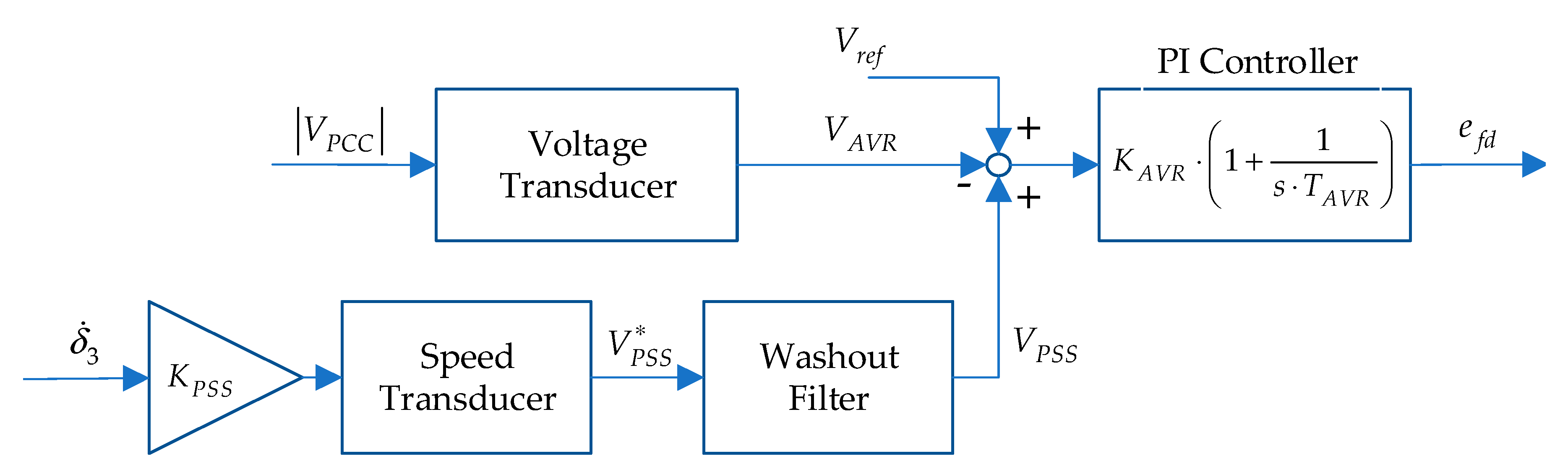
The model described by Equations (3) and (4) can be modified including the TG unit control loop. The SG excitation circuit is controlled by an Automatic Voltage Regulator (AVR) and a PSS in compliance with [22]. The transfer functions of the AVR and the PSS controllers are shown in Figure 3. The AVR regulates the SG field voltage e_fd with a PI controller whose proportional gain and time constant are denoted respectively as K_AVR and T_AVR. Usually, the AVR gain K_AVR has high value in order to provide the required air-gap torque when the rotational speed of the rotor ω_R deviates from the synchronous value. At very low frequencies (0–2 Hz), the action of the AVR could introduce undamped oscillations, hence the PSS action allows to avoid this instability source. The proportional gain of the PSS is denoted as K_PSS. $V_{AVR}$ denotes the signal provided in output by the voltage transducer. $V_{PSS}^{\ast }$ denotes the signal provided in output by the speed transducer. Differently $V_{PSS}$ denotes the output signal generated by the PSS.

Using the small-signal analysis, the grid voltage magnitude variation $\Delta \left|V_{PCC}\right|$ can be expressed as:

$$\Delta \left|V_{PCC}\right|=\frac{V_{PC{C}_{d0}}}{{\left|V_{PCC}\right|}_0}\cdot \Delta V_{PC{C}_d}+\frac{V_{PC{C}_{q0}}}{{\left|V_{PCC}\right|}_0}\cdot \Delta V_{PC{C}_q},$$

(5)

where $\Delta V_{PC{C}_d}$ and $\Delta V_{PC{C}_q}$ are the direct and quadrature component of the grid voltage vector; ${\left|V_{PCC}\right|}_0$, $V_{PC{C}_{d0}}$ and $V_{PC{C}_{q0}}$ are respectively the steady-state value of the grid voltage magnitude and the steady-state value of the direct and quadrature components.

The derivatives of the voltage signals related to the TG controllers can be calculated as:

$$\frac{d}{dt}\Delta V_{PSS}^{\ast }=\frac{1}{T{1}_{PSS}}\cdot \left(K_{PSS}\cdot \Delta {\delta }_3-\Delta V_{PSS}^{\ast }\right),$$

(6)

$$\frac{d}{dt}\Delta V_{PSS}=\frac{1}{T{1}_{PSS}}\cdot \left(K_{PSS}\cdot \Delta {\delta }_3-\Delta V_{PSS}^{\ast }\right)-\frac{1}{T{2}_{PSS}}\cdot \Delta V_{PSS},$$

(7)

$$\frac{d}{dt}\Delta V_{AVR}=\frac{K_R}{T_R}\cdot \left(\frac{V_{PC{C}_{d0}}}{{\left|V_{PCC}\right|}_0}\cdot \Delta V_{PC{C}_d}+\frac{V_{PC{C}_{q0}}}{{\left|V_{PCC}\right|}_0}\cdot \Delta V_{PC{C}_q}\right)-\frac{1}{T_R}\cdot \Delta V_{AVR},$$

(8)

where T1_PSS and T2_PSS are, respectively, the time constant of the speed transducer and the time constant of the washout filter; the gain and the time constant of the voltage transducer are indicated as K_R and T_R. The AVR and PSS control actions provide in output the signal $\Delta e_{fd}$ calculated as:

$$\Delta e_{fd}=K_{AVR}\cdot \left(\Delta V_{PSS}-\Delta V_{AVR}\right)+\frac{K_{AVR}}{T_{AVR}}\cdot \left({\displaystyle \int \Delta V_{PSS}}-{\displaystyle \int \Delta V_{AVR}}\right).$$

(9)

As a consequence the system defined in Equation (4) can be rearranged as:

$$\{\begin{array}{l}\frac{d}{dt}\Delta {\underset{\_}{\widehat{X}}}_{TG}={\widehat{A}}_{TG}\cdot \Delta {\underset{\_}{\widehat{X}}}_{TG}+{\widehat{B}}_{TG}\cdot \Delta {\underset{\_}{v}}_{PCC}+{\widehat{B}}_{TG}^{\ast }\cdot \Delta T_{GT}\\ \Delta {\underset{\_}{i}}_{SG}=C_{TG}\cdot \Delta {\underset{\_}{X}}_{TG}+D_{TG}\cdot \Delta {\underset{\_}{v}}_{PCC}\end{array},$$

(10)

with

$${\widehat{A}}_{TG}=\left[\begin{array}{cc}{A}_{TG}+B{2}_{TG}\cdot C_{TG}& A{1}_{FVC}\\ A{2}_{FVC}& A{3}_{FVC}\end{array}\right].$$

The state-space vector and the matrixes, which compose Equation (10), can be expressed as:

$$\Delta {\underset{\_}{\widehat{X}}}_{TG}={\left[\begin{array}{cccccc}\Delta {\underset{\_}{X}}_{TG}& \Delta V_{PSS}^{\ast }& \Delta V_{PSS}& {\displaystyle \int \Delta V_{PSS}}& \Delta V_{AVR}& {\displaystyle \int \Delta V_{AVR}}\end{array}\right]}^T,$$

(11)

$$A{1}_{FVG}=\left[\begin{array}{c}\left[0\right]\\ \begin{array}{ccccc}0& \frac{R_{fd}\cdot K_{AVR}\cdot {\omega }_R}{L_{ad}}& \frac{R_{fd}\cdot K_{AVR}\cdot {\omega }_R}{T_{AVR}\cdot L_{ad}}& -\frac{R_{fd}\cdot K_{AVR}\cdot {\omega }_R}{L_{ad}}& -\frac{R_{fd}\cdot K_{AVR}\cdot {\omega }_R}{T_{AVR}\cdot L_{ad}}\end{array}\\ \left[0\right]\end{array}\right],$$

(12)

$$A{2}_{FVC}={\left[\begin{array}{c}\left[0\right]\\ \begin{array}{ccccc}{K}_{PSS}/T{1}_{PSS}& K_{PSS}/T{1}_{PSS}& 0& 0& 0\end{array}\\ \left[0\right]\end{array}\right]}^T,$$

(13)

$$A{3}_{FVC}=\left[\begin{array}{ccccc}-1/T{1}_{PSS}& 0& 0& 0& 0\\ -1/T{1}_{PSS}& -1/T{2}_{PSS}& 0& 0& 0\\ 0& 1& 0& 0& 0\\ 0& 0& 0& -1/T_R& 0\\ 0& 0& 0& 1& 0\end{array}\right],$$

(14)

$${\widehat{B}}_{TG}={\left[\begin{array}{cccc}{\left(B{2}_{TG}\cdot D_{TG}\right)}^T& \left[0\right]& \begin{array}{c}\frac{V_{PC{C}_{d0}}}{{\left|V_{PCC}\right|}_0}\cdot \frac{K_R}{T_R}\\ \frac{V_{PC{C}_{q0}}}{{\left|V_{PCC}\right|}_0}\cdot \frac{K_R}{T_R}\end{array}& \left[0\right]\end{array}\right]}^T,$$

(15)

$${\widehat{B}}_{TG}^{\ast }=\left[\begin{array}{c}\left[0\right]\\ B_{TG}^{\ast }\end{array}\right].$$

(16)

Independently of the causes, in the presence of SSTI phenomena the generator shaft is led to vibrate. The overall damping of the TG unit coincides with the electrical damping since, as previously declared, the shaft-line inherent mechanical damping is assumed to be null. The TG electrical damping evaluation is based on the matrix Â_TG eigenvalues calculation. Besides the torsional natural frequencies of the shaft-line can be identified. In particular, Equation (10) allows one to detect two modes of torsional vibration for each TG with TNFs equal to 9.2 and 31.5 Hz.

The TG units rated electrical and torsional mechanical parameters are reported respectively in

Table 1. TG units’ electrical parameters.

Parameter	Value	Unit
TG rated power	44	MVA
TG rated line to line voltage	11	KV
TG rated frequency	50	Hz
SG stator resistance ($R_a$)	0.0024	pu
SG rotor resistances (${R^{\prime }}_{fd}$, ${R^{\prime }}_{kd}$, ${R^{\prime }}_{kq}$)	0.0006, 0.04, 0.02	pu
SG d-q magnetizing inductance ($L_{ad}$, $L_{aq}$)	1.63, 0.81	pu
SG winding leakage inductance ($L_l$)	0.1	pu
SG rotor inductances (${L^{\prime }}_{fd}$, ${L^{\prime }}_{kd}$, ${L^{\prime }}_{kq}$)	0.14, 0.08, 0.14	pu

and

Table 2. TG units’ mechanical parameters.

Parameter	Value	Unit
Inertia coefficients ($J_1$, $J_2$ and $J_3$)	9.166, 1.461, 2.764	pu
Stiffness coefficients ($K_1$ and $K_2$)	135.273, 27.235	pu
First torsional natural Frequency (TNF1)	9.2	Hz
Second torsional natural Frequency (TNF2)	31.5	Hz

.

The sensitivity analysis can be applied to detect the TG control parameters, which impact the torsional stability of the electromechanical system. The Finite Difference Method (FDM) [18] can be adopted to provide the sensitivity analysis of the system shown in Figure 2. FDM implies simple implementation and computational burden proportional to the number of design variables.

Considering the objective function F(P) as a function of a design variable P, its sensitivity coefficient can be approximated from the exact displacement between the initial point P₀ and the perturbated point P₀ + ΔP, where ΔP is the perturbation of the design variable.

Accuracy can be improved using the central-difference approximation and the sensitivity coefficient dF/dP can be defined as:

$$\frac{dF}{dP}=\frac{F\left(P_0+\Delta P\right)-F\left(P_0-\Delta P\right)}{2\Delta P}.$$

(17)

As discussed in [23] the FDM approximation can lead to an accuracy error, which can be reduced by a proper choice of the perturbation ΔP. In order to reduce the error source, the perturbation ΔP can be assumed high, in particular 50% of the considered design variable.

Considering the data shown in Table 1 and Table 2, the sensitivity analysis can be applied to the state-space electromechanical model of the TG units. The analysis is performed assuming rated conditions of the TG unit and starting from the controller parameters provided by the Original Equipment Manufacturers (OEMs) and reported in

Table 3. TG units’ control system parameters.

Parameter	Value	Unit
AVR proportional gain KAVR	15	pu
AVR integral time constant TAVR	8	s
Voltage transducer cut-off frequency	30	Hz
PSS proportional gain KPSS	1	pu
PSS time constant T1PSS	0.02	s
PSS time constant T2PSS	1.5	s

.

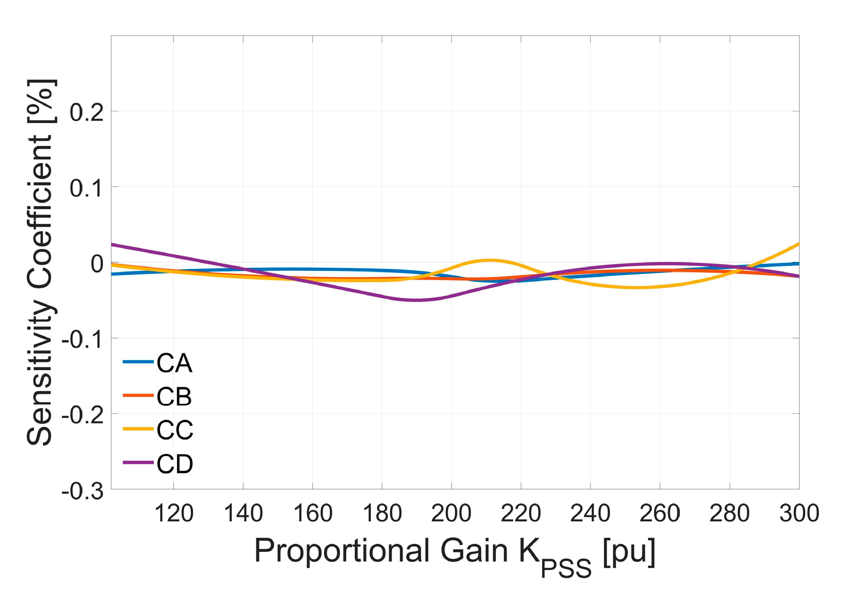
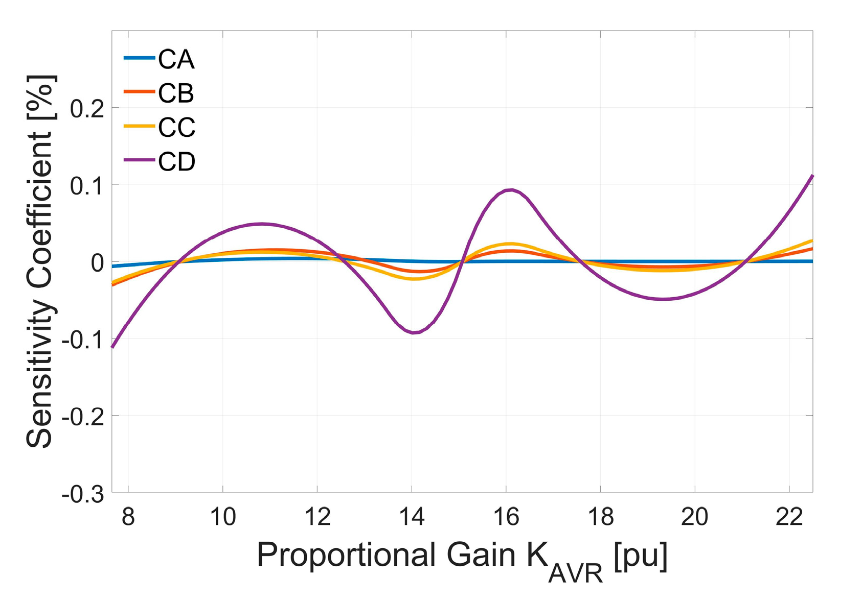
On the basis of Equation (17) the FDM analysis can be carried out regarding various frequencies. The sensitivity coefficients for the phase and the magnitude of the output current perturbations $\Delta {\underset{\_}{i}}_{SG}$ can be determined considering the action of the AVR and the PSS controllers. The magnitude sensitivity coefficients provide percent information about $\Delta {\underset{\_}{i}}_{SG}$ magnitude variation due to the controller’s parameters variation in respect of the steady-state conditions. The phase sensitivity coefficients provide information about $\Delta {\underset{\_}{i}}_{SG}$ phase variation expressed in degrees.

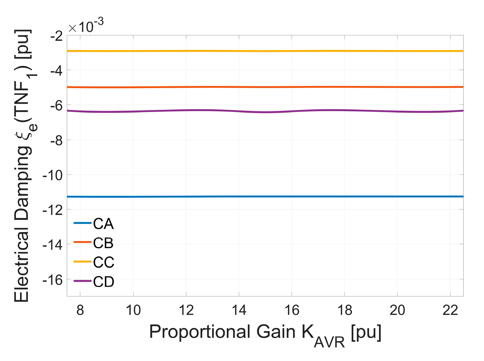
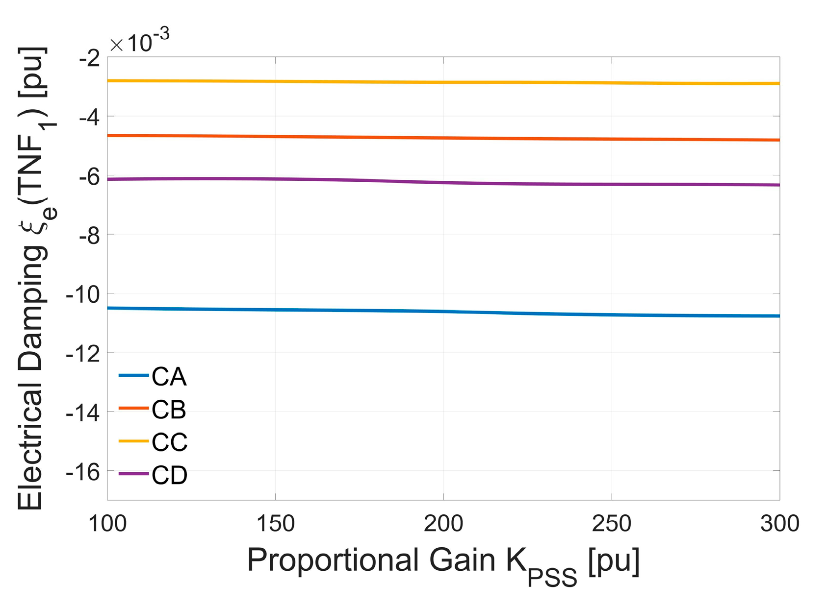
The sensitivity coefficients related to the AVR and PSS control parameters were calculated and the results point out that the AVR and PSS proportional gains (K_AVR and K_PSS) had more impact than the other design parameters (T_AVR, T1_PSS and T2_PSS). Nevertheless, also the sensitivity coefficients related to the AVR and PSS proportional gains variations were very low as shown in

Table 4. TG unit controller’s sensitivity coefficients.

Sensitivity Coefficients Related to KPSS Variation
Frequency [Hz]	Magnitude [%]	Phase [Degree]
5 Hz	−3.5	0
10 Hz	−1.0	0
15 Hz	−1.0	0
30 Hz	−0.5	0
50 Hz	0	0
Sensitivity coefficients related to KAVR variation
Frequency [Hz]	Magnitude [%]	Phase [Degree]
5 Hz	17.0	0
10 Hz	10.5	0
15 Hz	5.5	0
30 Hz	2.5	0
50 Hz	1.5	0

. Considering the frequency range 5–50 Hz, the torsional stability seemed not influenced by the AVR and the PSS proportional gains variations since the phase of $\Delta {\underset{\_}{i}}_{SG}$ did not vary with K_AVR or K_PSS and the magnitude of $\Delta {\underset{\_}{i}}_{SG}$ was subjected to low value changes. Considering, for example, the data at 10 Hz, the increase of 50% of K_AVR or K_PSS led the current $\Delta {\underset{\_}{i}}_{SG}$ to increase its magnitude about 10 percent or to decrease about 1 percent, respectively.

4. TVFD Complete Model

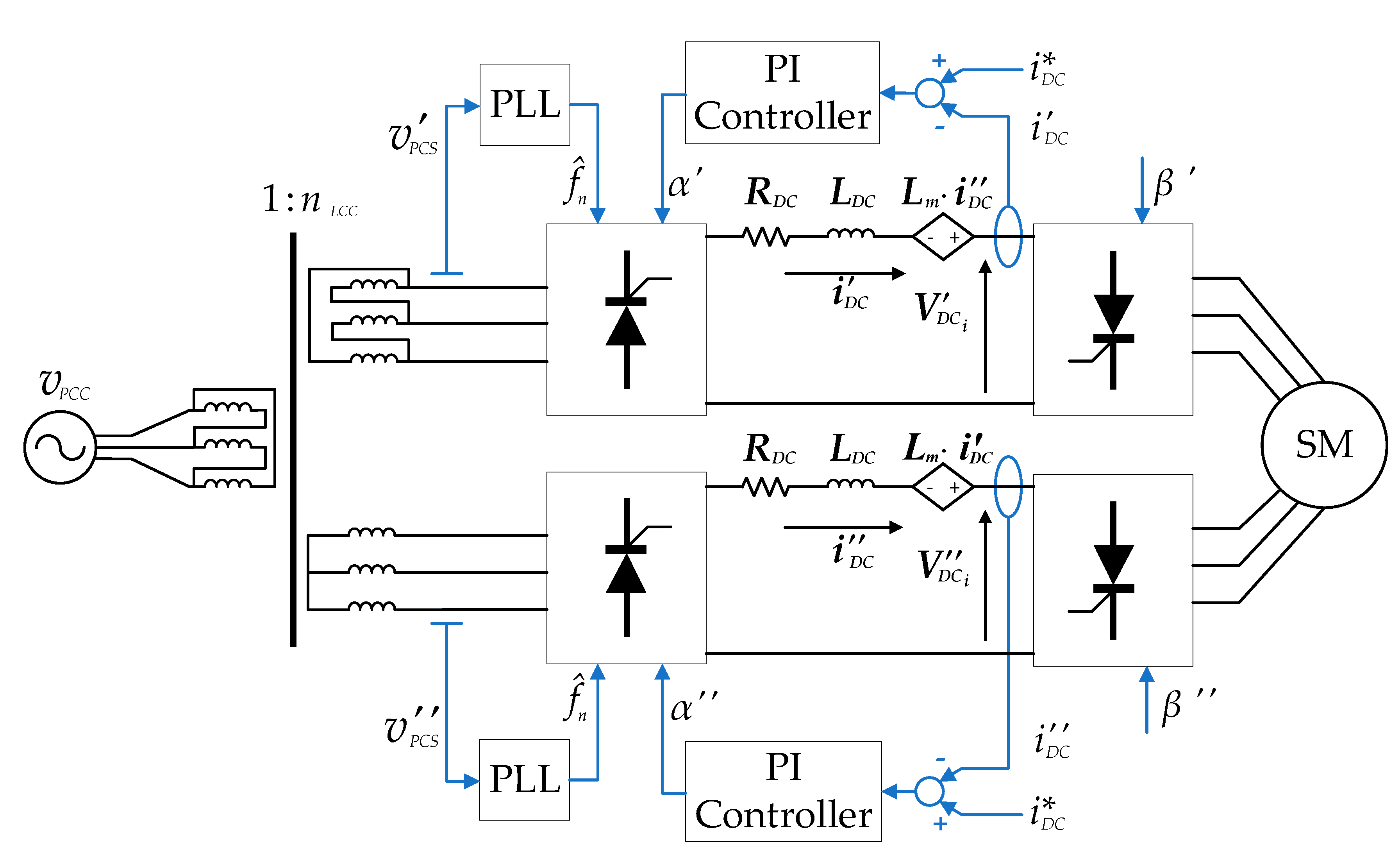
The detailed structure of the PCSs shown in Figure 1 is represented in Figure 4. Each TVFD consists of two branches whose DC-links are coupled by the mutual inductance L_m. The control scheme of the TVFD first stage is depicted in the same figure where ${V^{\prime }}_{D{C}_i}$ and ${V^{″}}_{D{C}_i}$ denote the DC-links output voltages. The DC link currents are controlled by means of two PI controllers, which set the firing angles α′ and α″. Differently the TVFD second stage operates with constant firing angles denoted as β′ and β″. Two Phase Locked Loops (PLLs) provide synchronization with the voltages ${v^{\prime }}_{PCC}$ and ${v^{″}}_{PCC}$ and estimate the grid frequency ${\widehat{f}}_n$.

In [1] the state-space model of the TVFD first power conversion stage has been presented and based on small-signal linearization. The operation of the power conversion stage can be defined by the following equation.

$$\{\begin{array}{l}\frac{d}{dt}\Delta {\underset{\_}{i}}_{DC}=A_{VFD}\cdot \Delta {\underset{\_}{i}}_{DC}+\left[\begin{array}{ccc}B{1}_{VFD}& B{2}_{VFD}& B{3}_{VFD}\end{array}\right]\cdot {\left[\begin{array}{ccc}\Delta {\underset{\_}{v}}_{PCC}& \Delta {\underset{\_}{V}}_{D{C}_i}& \Delta \underset{\_}{\alpha }\end{array}\right]}^T\\ \left[\begin{array}{c}\Delta {\underset{\_}{i}}_{DC}\\ \Delta {\underset{\_}{i}}_{PCS}\end{array}\right]=C_{VFD}\cdot \Delta {\underset{\_}{i}}_{DC}\end{array},$$

(18)

where the inputs are the PCC voltage fluctuations $\Delta {\underset{\_}{v}}_{PCC}$, the variations of the DC-links voltages $\Delta {\underset{\_}{V}}_{D{C}_i}$ and the variations of the firing angles $\Delta \underset{\_}{\alpha }$ related to the two LCRs; $\Delta {\underset{\_}{i}}_{PCS}$ is the vector of the current perturbations and $\Delta {\underset{\_}{i}}_{DC}$ is the vector of DC currents variations.

The coefficients of Equation (18) are defined as:

$$A_{VFD}=\frac{1}{\Delta T}ln\left(\frac{\delta {\underset{\_}{X}}_5(t_1)}{\delta {\underset{\_}{X}}_1(t_0)}\right),$$

(19)

$$B{1}_{VFD}={\left(\frac{\delta {\underset{\_}{X}}_5(t_1)}{\delta {\underset{\_}{X}}_1(t_0)}-1\right)}^{-1}\cdot A_{VFD}\cdot \frac{\delta {\underset{\_}{X}}_5(t_1)}{\delta {\underset{\_}{v}}_{PCC}},$$

(20)

$$B{2}_{VFD}={\left(\frac{\delta {\underset{\_}{X}}_5(t_1)}{\delta {\underset{\_}{X}}_1(t_0)}-1\right)}^{-1}\cdot A_{VFD}\cdot \frac{\delta {\underset{\_}{X}}_5(t_1)}{\delta {\underset{\_}{V}}_{D{C}_i}},$$

(21)

$$B{3}_{VFD}={\left(\frac{\delta {\underset{\_}{X}}_5(t_1)}{\delta {\underset{\_}{X}}_1(t_0)}-1\right)}^{-1}\cdot A_{VFD}\cdot \frac{\delta {\underset{\_}{X}}_5(t_1)}{\delta \underset{\_}{\alpha }},$$

(22)

$$C_{VFD}={\left[\begin{array}{ccc}\begin{array}{cc}1& 0\\ 0& 1\end{array}& T_1\cdot P\left(\theta \right)& T_1\cdot P\left(\theta \right)\end{array}\right]}^T,$$

(23)

where ΔT denotes the TVFD commutation period; X₅ is the state-space vector when the commutation process is assumed completed, t₀ denotes the initial time instant of the first commutation stage; t₁ denotes the end of the commutation period; P(θ) is the Park transformation matrix and θ is the Park angle. Further details can be found in [1].

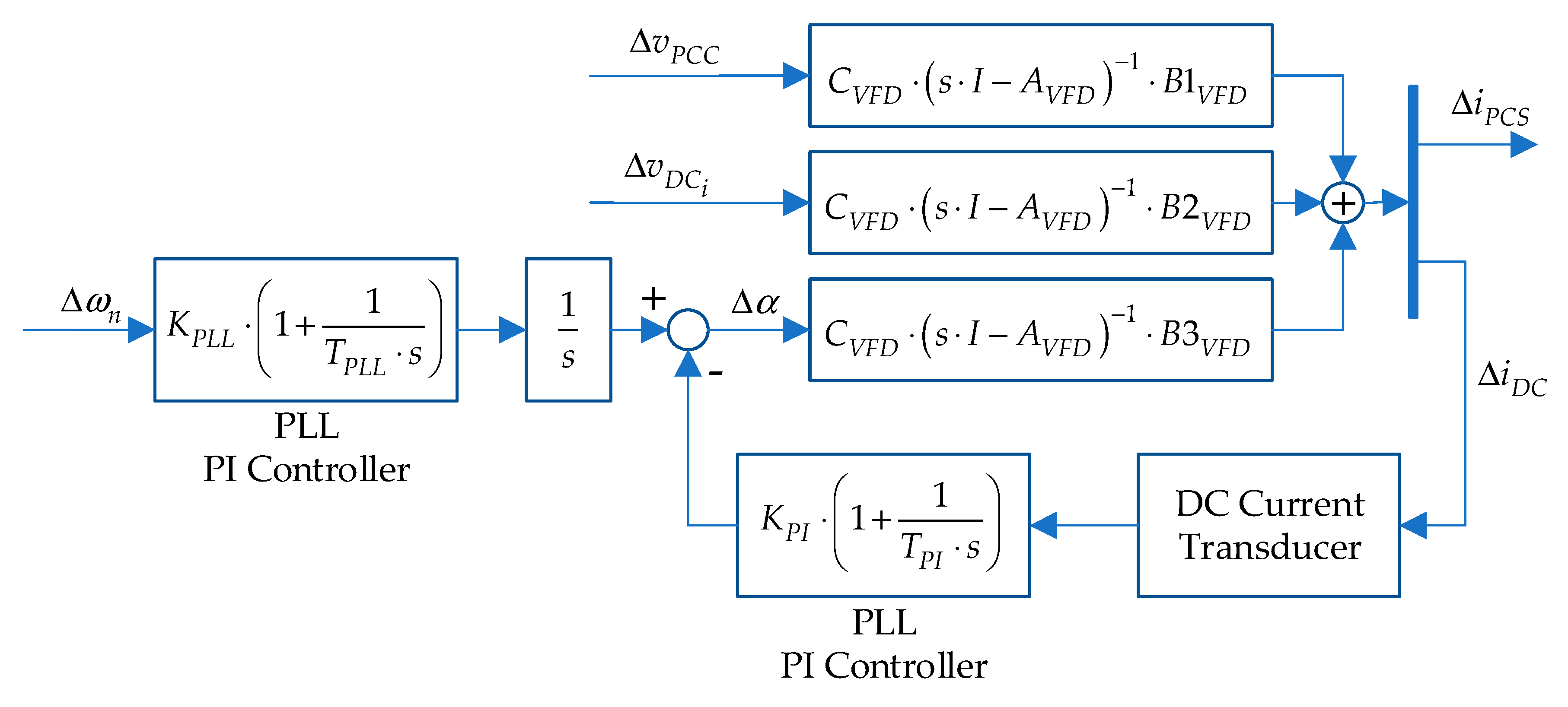
Since the SSTI phenomena are strongly influenced by the TVFD controller parameters [2], a more detailed TVFD model can be developed where the current controllers and the PLLs dynamics can be included. The detailed control scheme of the TVFD and the PLL structure are shown respectively in Figure 5 and Figure 6 where K_PI and T_PI denote the proportional gain and the time constant of the DC current controllers while K_PLL and T_PLL denote the proportional gain and the time constant of the PLL PI.

The closed-loop state-space model is described by the following equations system:

$$\{\begin{array}{l}\frac{d}{dt}\Delta {\underset{\_}{X}}_{PCS}=A_{PCS}\cdot \Delta {\underset{\_}{X}}_{PCS}+B_{PCS}\cdot {\left[\begin{array}{ccc}\Delta {\underset{\_}{v}}_{PCC}& \Delta {\underset{\_}{V}}_{D{C}_i}& \Delta {\omega }_n\end{array}\right]}^T\\ \Delta {\underset{\_}{i}}_{PCS}=C_{PCS}\cdot \Delta {\underset{\_}{X}}_{PCS}\end{array}.$$

(24)

where the state-space vector ΔX_PCS includes the vector of DC currents, the dynamics of the PLLs and the dynamics of the PI current controllers.

The inputs of the state-space (24) are the PCC voltage fluctuations $\Delta {\underset{\_}{v}}_{PCC}$, the DC-links voltages variations $\Delta {\underset{\_}{V}}_{D{C}_i}$ and the variations of grid pulsation $\Delta {\omega }_n$.

The PCSs rated parameters and the control parameters provided by the OEMs are reported respectively in

Table 5. PCSs parameters.

Parameter	Value	Unit
TVFD rated power	17.4	MVA
TVFD rated DC current	1692	A
LCR rated line to line voltage	4.75	kV
LCI rated line to line voltage	4.2	kV
LCI rated firing angle	37.8	degree
Motor stator resistance RM and sub synchronous reactance LM	0.00098, 0.1033	pu
Motor frequency	60	Hz
Grid frequency	50	Hz
DC-links resistance RDC	0.0057	pu
DC-links inductance LDC	0.8480	pu
DC-links mutual inductance Lm	−0.5088	pu

and

Table 6. TVFD controller’s parameters.

Parameter	Value	Unit
Current controller proportional gain KPI	0.18	pu
Current controller integral time constant TPI	0.025	s
DC Filter damping factor ξDC	0.707	pu
DC Filter cut-off pulsation ωDC	314.15	rad/s
PLL proportional gain KPI	10	pu
PLL integral time constant TPI	0.33	s

.

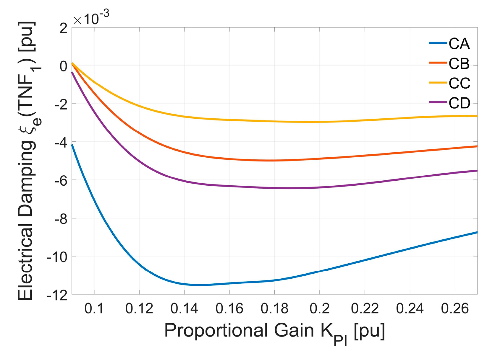
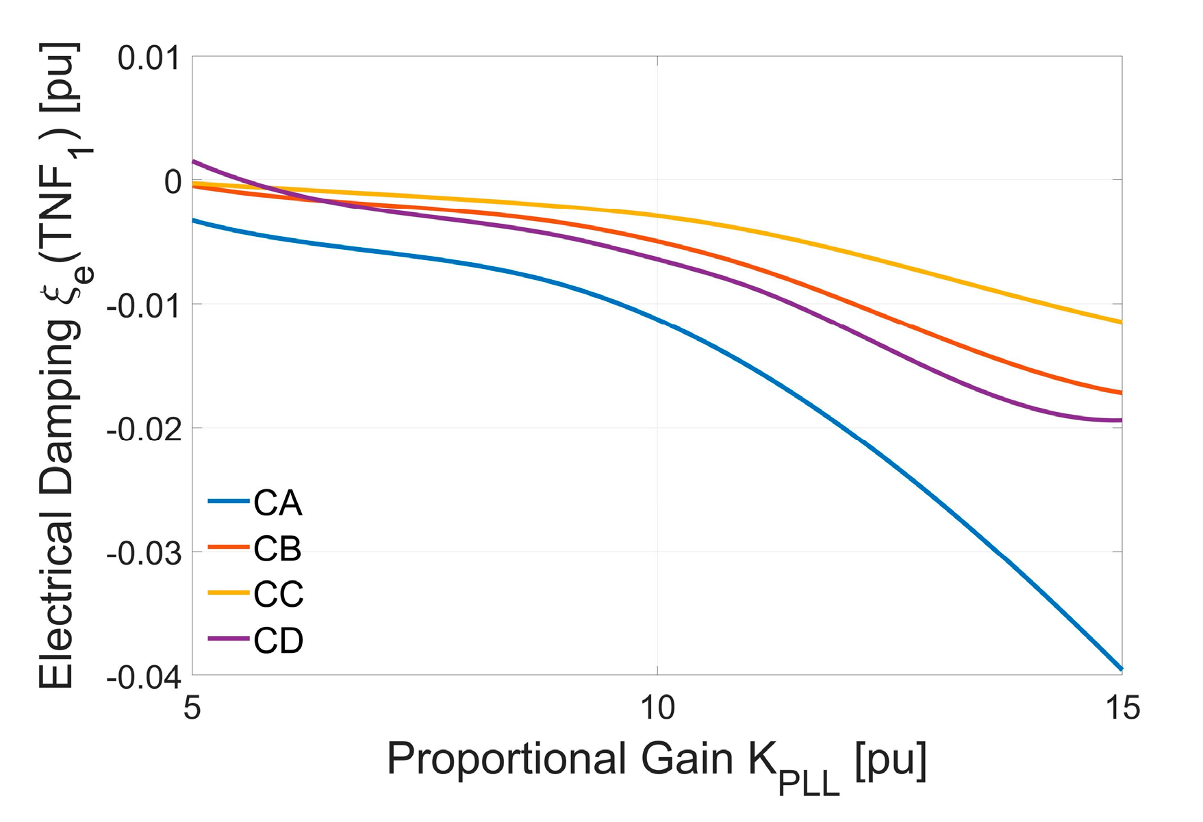
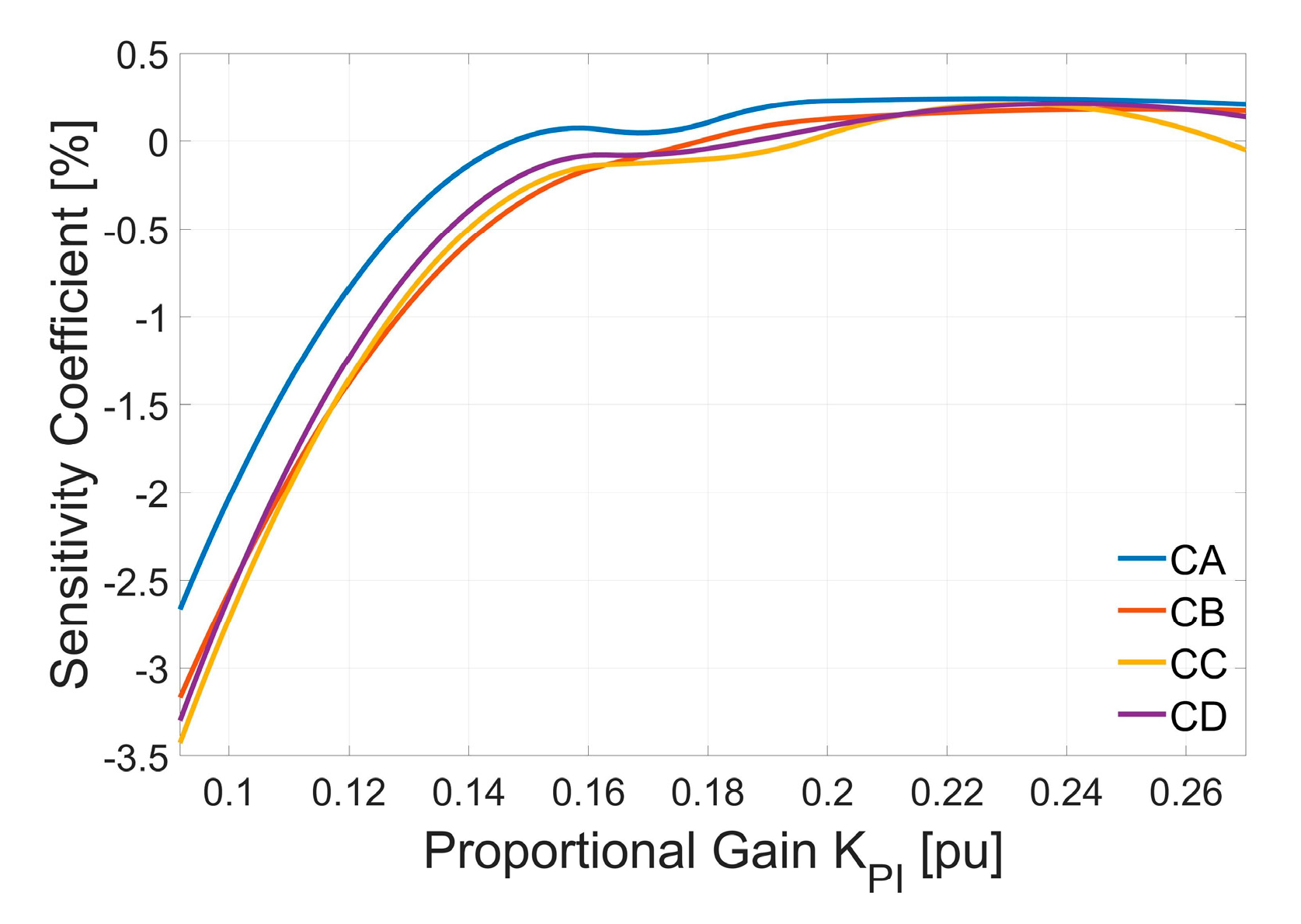
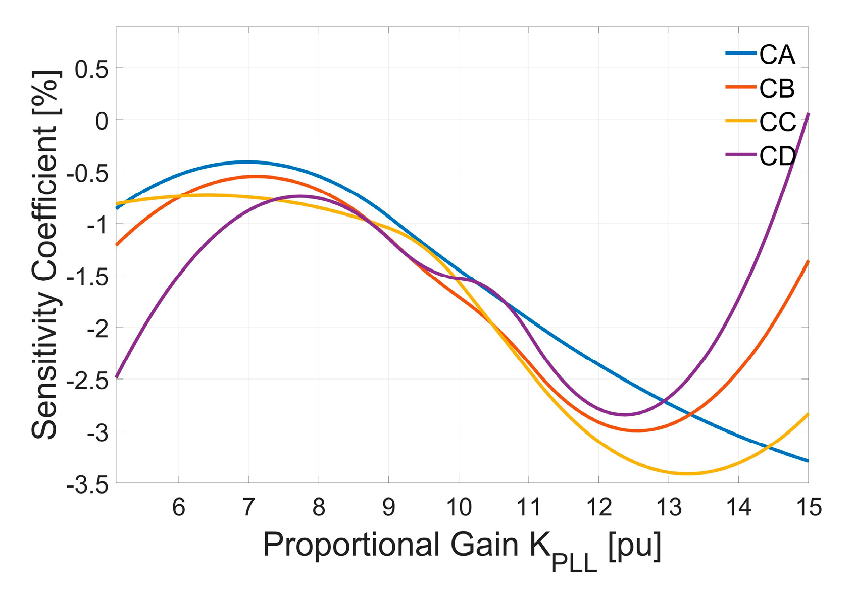
The FDM analysis can be applied to the model described by Equation (24) in order to assess the control parameters that influence the stability of the overall power system. On the basis of Equation (17) the FDM analysis is carried out regarding various frequencies. The sensitivity coefficients for the phase and the magnitude of the output current perturbations $\Delta {\underset{\_}{i}}_{PCS}$ can be determined considering the action of the PI current controllers and of the PLLs. The parameters K_PI and K_PLL are detected as elements with high sensitivity coefficients.

The magnitude sensitivity coefficients provide percent information about $\Delta {\underset{\_}{i}}_{PCS}$ magnitude variation due to the controller’s parameters variation in respect to the steady-state conditions. The phase sensitivity coefficients provide information about $\Delta {\underset{\_}{i}}_{PCS}$ phase variation expressed in degrees.

The data reported in

Table 7. TVFD controller’s sensitivity coefficients.

Sensitivity Coefficients Related to KPI Variation
Frequency [Hz]	Magnitude [%]	Phase [Degree]
5 Hz	58.5	30.0
10 Hz	10.5	20.0
15 Hz	9.5	15.0
30 Hz	7.5	2.5
50 Hz	3.5	0
Sensitivity Coefficients Related KPLL Variation
Frequency [Hz]	Magnitude [%]	Phase [Degree]
5 Hz	-3.5	10.0
10 Hz	-1.0	10.0
15 Hz	-1.0	5.0
30 Hz	0	0
50 Hz	0	0

point out that the sensitivity coefficients decrease when the frequency increases. At high frequencies the variations of K_PI and K_PLL are not able to influence the magnitude or the phase of $\Delta {\underset{\_}{i}}_{PCS}$. At frequencies close to the TG first TNF (9.2 Hz) the sensitivity coefficients are indicative. Differently from the results reported in Table 4, the phase coefficients are significant about the TVFD controller’s parameters. Considering, for example, the data at 10 Hz, a 50% variation of K_PI or K_PLL leads to a phase shift of the current perturbations $\Delta {\underset{\_}{i}}_{PCS}$ equal to 20 degree or 10 degree, respectively.

5. LNG Plant Simulation Platform

The theoretical model described in Section 3 and Section 4 allows one to obtain electrical damping assessment and stability considerations in case of a basic LNG plant, which consists of a TG unit and a TVFD. In order to manage complex plant configurations, a complete simulation platform has been developed using the software DigSILENT PowerFactory, which allows one to provide detailed simulation results in the time domain. 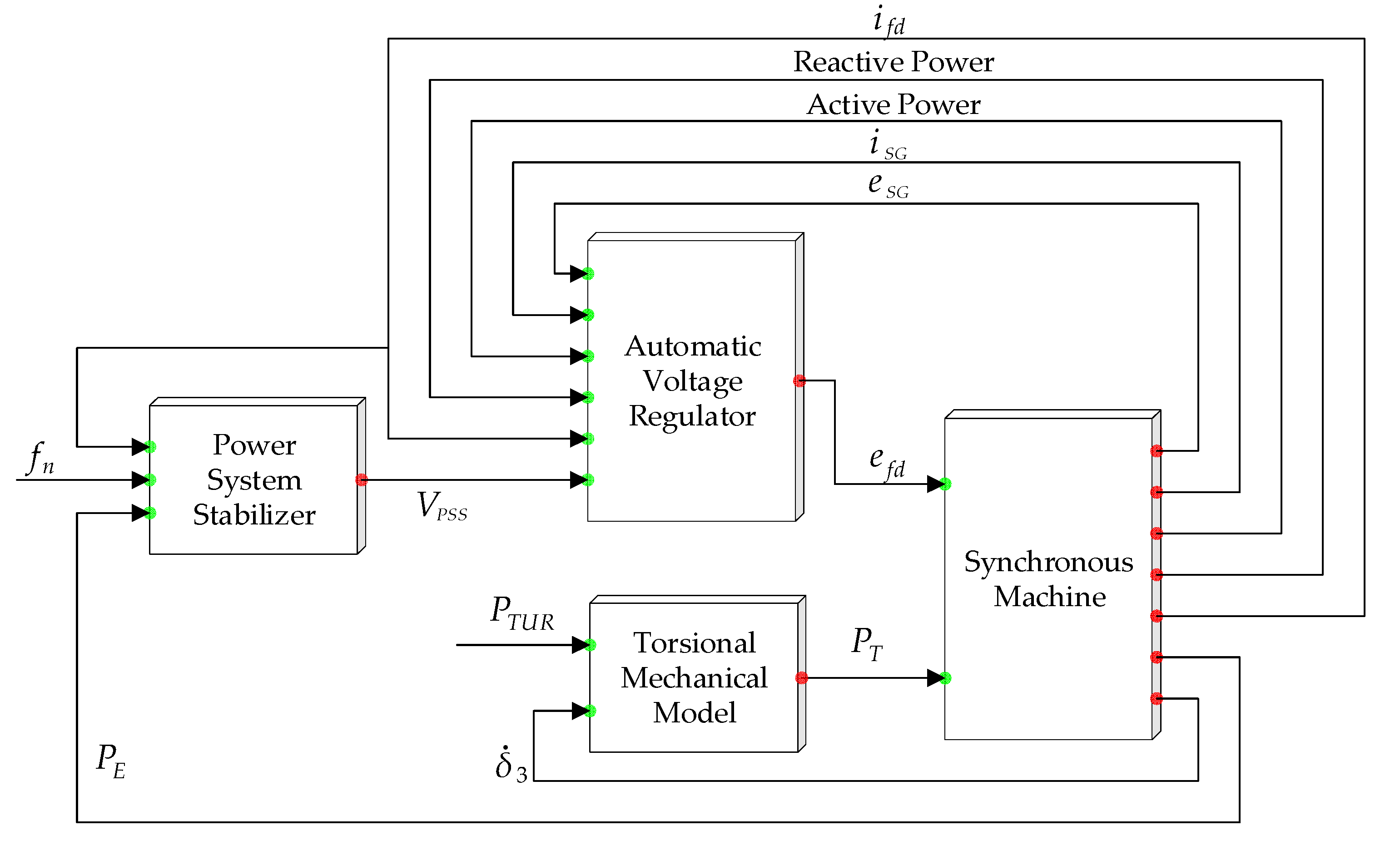The overall power system shown in Figure 1 has been emulated. In Figure 7 there is represented the scheme of the TG unit integrated model used for the implementation in DigSILENT environment while the TVFD implementation is based on Figure 4.

The TG unit was emulated considering the torsional mechanical model and the control system discussed in Section 3. The SG was modeled through a classic d–q representation provided by the Power Factory software. In Figure 7 the powers related to the TG shaft torque, the air-gap-torque and the driving torque of the TG were indicated respectively with P_T, P_E and P_TUR.

The PCSs and their control system were implemented on the basis of the model discussed in Section 4. The motor M of each compression train was represented as an ideal voltage source connected to the subsynchronous reactance L_M and the stator resistance R_M.

The TVFDs models and the TG units models were connected in order to obtain a combined electromechanical model. The action of the filter HF was taken into account since it modifies the operative condition of the TG units, changing the amount of active and reactive power supplied by the SGs. The MV transformers were modeled on the basis of their short circuit voltages and the Joule losses. The step-up transformers related to the TG units (TTG1, TTG2 and TTG3) were assumed identical such as the step-down transformers related to the TVFDs (TPCS1 and TPCS2). The transformers parameters are reported in

Table 8. Transformers electrical parameters.

Parameter	Value	Unit
TTG1,2,3 Rated Voltage	30/4.75/4.75/6	kV
TTG1,2,3 Sub-synchronous Reactance	0.0026	pu
TTG1,2,3 Joule Losses	0.01	%
TPCS1,2 Rated Voltage	11/30	kV
TPCS1,2 Sub-synchronous Reactance	0.00026	pu
TPCS1,2 Joule Losses	0.005	%

.

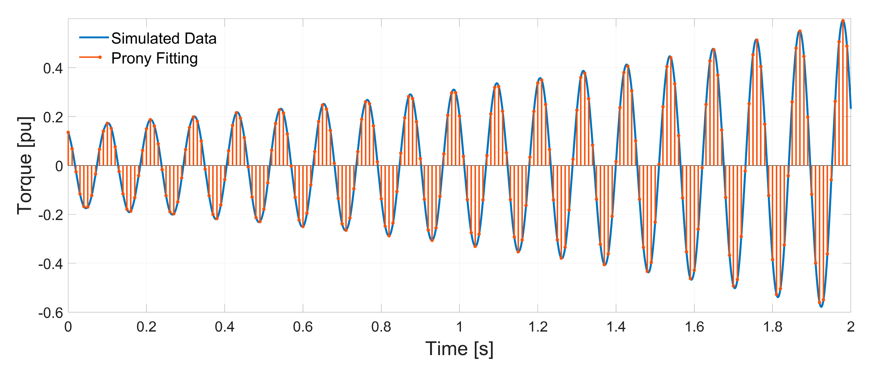
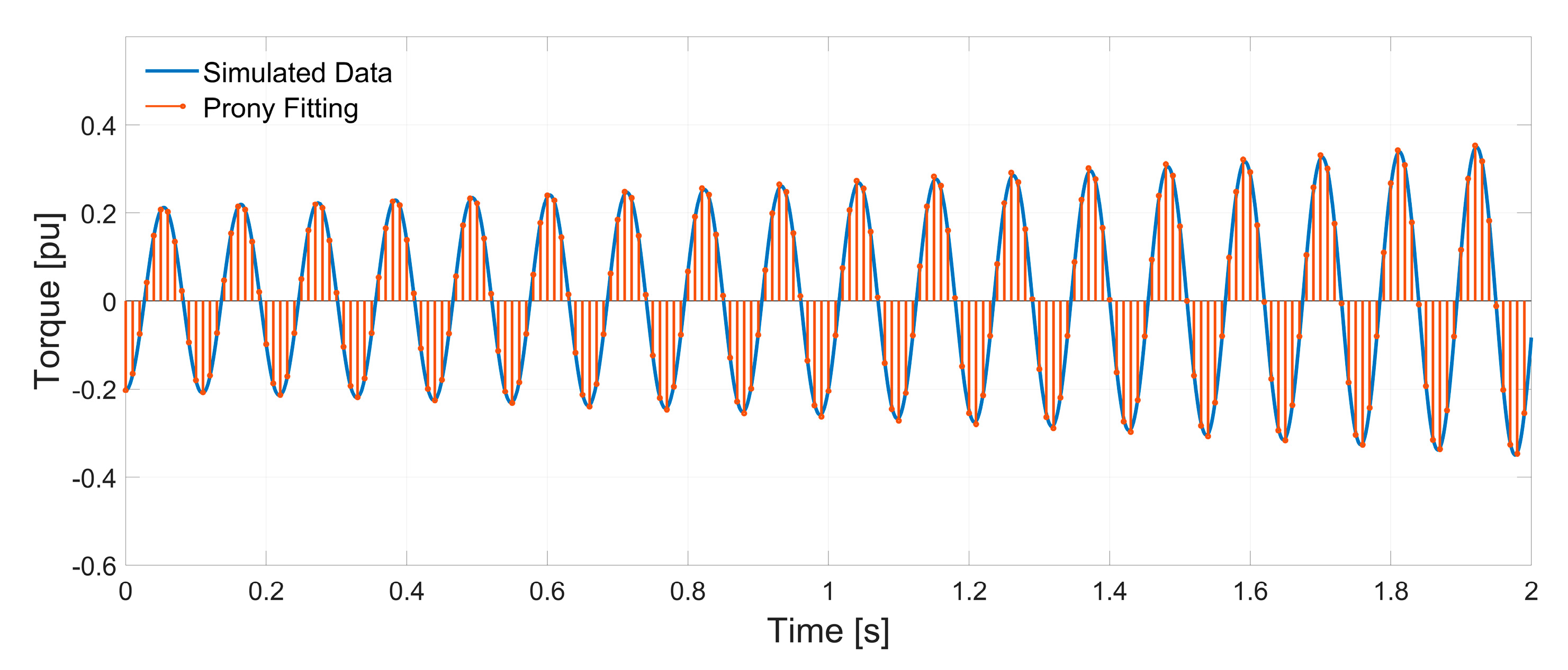
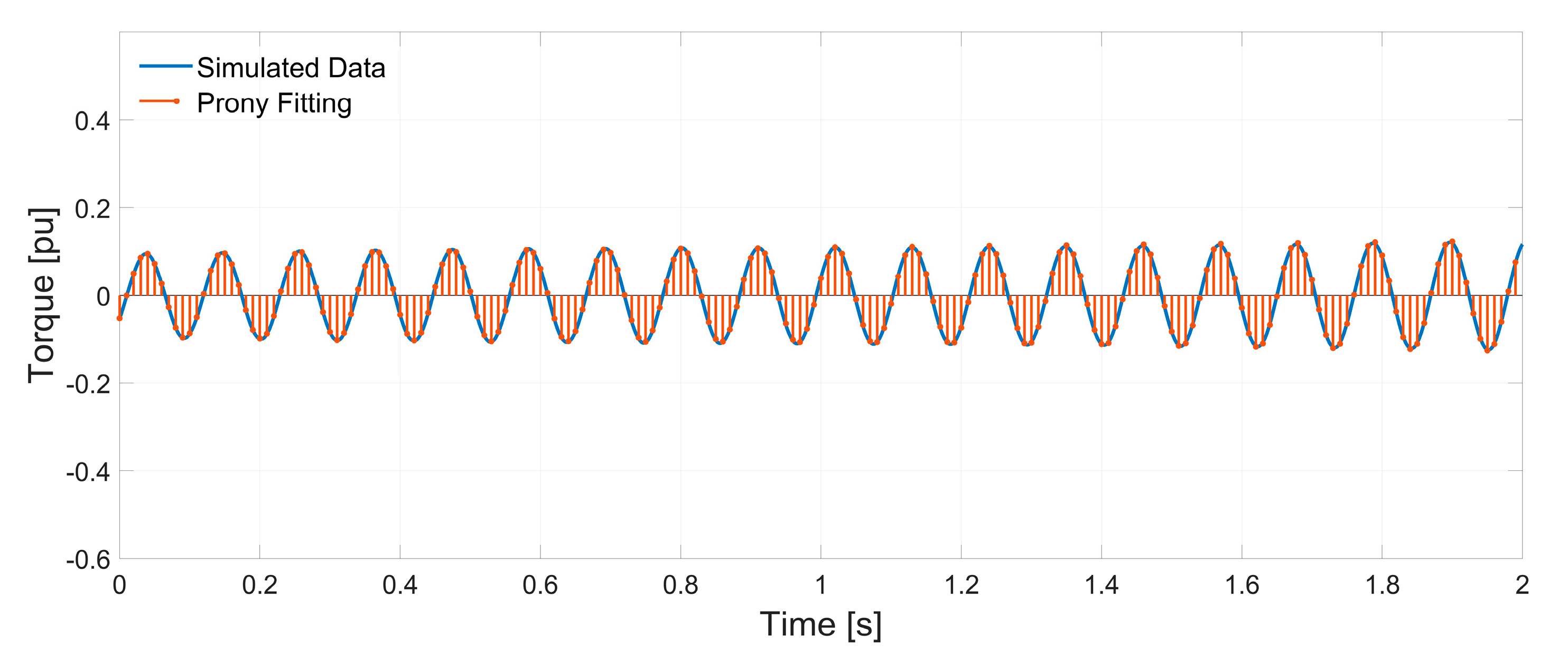
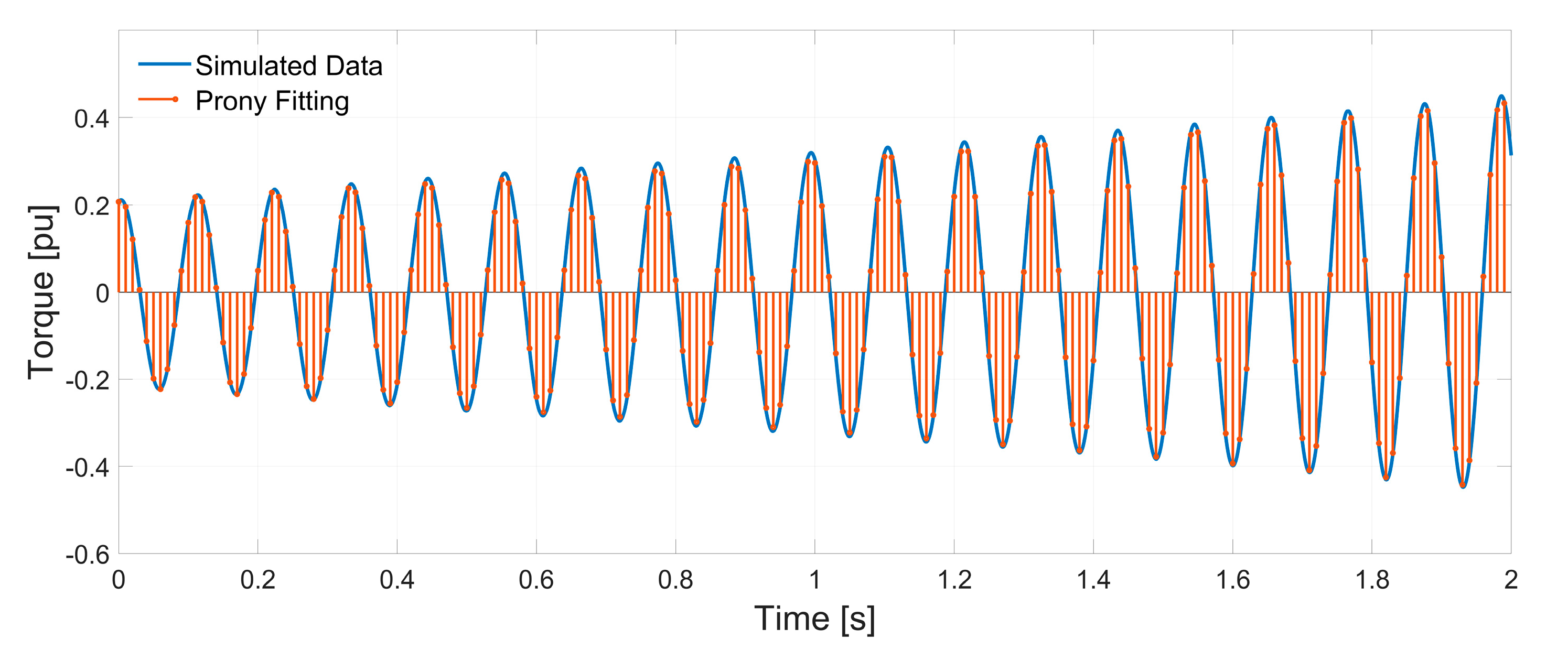
The TG shaft-line torque signals provided by the simulation platform are typically affected by time varying components in transient conditions. For this reason the torque signals can be post-processed through the Prony analysis as already discussed in [1]. In particular, the Prony analysis allows one to identify growing or decaying components of a generic signal f(t) on the basis of the following equation:

$$f(t)={\displaystyle {\sum }_{g=1}^N{K}_g\cdot e^{{\omega }_g\cdot {\xi }_g\cdot t}\cdot cos({\omega }_g\cdot t)},$$

(25)

where K_g is the magnitude, ξ_g is the damping factor, ω_g is the pulsation and g is an integer.

Considering the case study shown in Figure 1, the results provided by the developed LNG plant simulation platform were post-processed through the Prony analysis and successively a proper estimation of the damping factor ξ(f_i) was achieved for each TG unit. The stability assessment of the LNG plant and the sensitivity analysis are direct consequences.

6. Simulation and Experimental Results

A real LNG plant was used as an experimental set-up to carry on an extensive experimental tests campaign. The electrical and mechanical parameters of the experimental set-up were already reported in Table 1, Table 2 and Table 3 and Table 5, Table 6 and Table 8. The data obtained by the experimental measurements were compared and combined with the simulation results in order to provide a damping assessment of the considered LNG plant. Finally, the simulation platform results were used to perform a sensitivity analysis about the main control systems parameters. The impact of the control system parameters on the TG units overall damping was evaluated and the results could be applied to operate the LNG plant avoiding conditions with high risk of torsional instability.

6.1. Experimental Set-Up Configuration

Looking at the LNG plant shown in Figure 1, the three TG units and their control systems were identical. Additionally, the two moto-compressor trains and the related PCSs were assumed equal. The main components of the experimental set-up are shown in Figure 8 and Figure 9. The speed of the TG units and of the moto-compressor trains was measured by a magnetic pick-up.

In the LNG plant, a Torsional Monitoring System (TMS) was included. It allows one to provide as an output the angular oscillation of the turbine toothed wheel at the point of measurement [24]. The resulting alternating torque was calculated on the basis of the detailed torsional model of the shaft-line.

The SGs stator voltages and currents were measured respectively by means of voltage transformers (VTs) and current transformers (CTs). Probes installed inside the AVR system provide the voltage and the current measurements of the SGs field circuits (Figure 8).

With reference to the PCSs and the moto-compressor trains, the following measurements were available: DC-link’s currents, LCR’s firing angles, LCI’s firing angles, LCR’s AC voltages and motor’s voltages (Figure 9).

Considering the real LNG plant, the torsional vibration measurements on the TG unit were not available during the first phases of the set-up commissioning. The TMS was installed after the occurrence of the first SSTI phenomena. However, the torsional oscillations of the TG units can be evaluated also by the analysis of the DC-link’s currents. Indeed, the currents measured at the DC-links of the TVFDs can be used to estimate the overall damping ξ(TNF₁) related to the first TNF. In particular the spectra of DC-link currents can be obtained using the Continuous Wavelet Transform (CWT) [25]. Then, the component related to the first TNF of the TG can be extracted.

The magnitude of the component at the first TNF can be also approximated through the function $i_{DC}(TN{F}_1)$ expressed as:

$$i_{DC}(TN{F}_1)=A_{TNF1}\cdot e^{-2\cdot \pi \cdot TN{F}_1\cdot \xi \left(TN{F}_1\right)},$$

(26)

where A_TNF1 is the initial value of the current oscillation. Further details can be found in Appendix B.

Hence, the overall damping ξ(TNF₁) is estimated comparing $i_{DC}(TN{F}_1)$ (Equation (26)) with the DC-link current component at the first TNF provided by the spectrum.

Finally the derivative-free optimization method [26] can be used to identify the value of ξ(TNF₁), which minimizes the difference between the component extracted by the spectrum and the approximation defined by Equation (26).

6.2. Damping Assessment

Considering the experimental set-up shown in Figure 8 and Figure 9 and the LNG plant simulation platform discussed in Section 5, four different Configurations (Cs) are analyzed and denoted as CA, CB, CC and CD. The Cs mainly differ in the number of TG units connected to PCC, the power of the lumped load and the PCSs number. The main data related to the four configurations are reported in

Table 9. Experimental configurations of the LNG plant.

	CA	CB	CC	CD
Number of TGs	1	2	3	3
Number of PCSs	1	1	1	2
TVFD1 power [pu]	0.45	0.45	0.45	0.90
TVFD2 power [pu]	0	0	0	0.50
Compression train speed [rad/s]	240	363	363	377
Lumped load power [MW, MVAr]	11, 4	12, 2.3	12, 2.3	12, 2.3
Power per TG [pu]	0.54	0.29	0.19	0.34

.

In the proposed analysis the mechanical damping related to the four Cs was estimated subtracting the electrical damping calculated by the simulations results from the overall damping calculated by the experimental results.

The spectrum of the DC-link current ${i^{\prime }}_{DC}$ was used to extract the component related to the first TNF as discussed previously. Figure 10, Figure 11 and Figure 12 show the spectra of ${i^{\prime }}_{DC}$ in the frequency range (0–100 Hz) related to the configurations CA, CB and CD. As expected, the ${i^{\prime }}_{DC}$ spectra show that, apart from the direct component, the component at the first TNF exhibited the highest value and it grows with the time.

In Figure 13, Figure 14 and Figure 15 the components measured at the first TNF were compared with the approximate curves obtained by Equation (26) and represented as dotted lines. A very good match between the two curves was verified in configuration CA (Figure 13). This provides also information about the proper calculation of the overall damping. The smaller overlap was verified in the case of configurations CB and CD (Figure 14 and Figure 15). This is due to the presence of more TG units, which have the same frequency but operate not exactly in phase. However, in all the examined configurations, Equation (26) guarantees satisfying approximation of the ${i^{\prime }}_{DC}$ component at the TNF. As a consequence, also the overall damping related to the TG units was estimated accurately.

The results related to the configuration denoted as CC were not reported since, in this case, the first TNF component of the current ${i^{\prime }}_{DC}$ exhibited a very low value.

Figure 16, Figure 17, Figure 18 and Figure 19 show the shaft-line torques related to the first TG unit in configurations CA, CB, CC and CD respectively. The results were obtained by the simulation platform and they are post-processed through the Prony analysis. The simulations are performed assuming zero mechanical damping and stressing the shaft line of one TG unit with a torque impulse. In this hypothesis the overall damping was calculated using Equation (25) and the overall damping was assumed equal to the electrical component. The fine overlap between the simulation results and Prony curves indicates a good approximation of the electrical damping calculation.

Starting from the overall damping estimated by the experimental measurements and through Equation (26), the mechanical damping related to the four configurations could be evaluated subtracting the electrical damping from the overall damping. The results are summarized in

Table 10. Overall, electrical and mechanical damping.

	CA	CB	CC	CD
Overall Damping ξ(TNF1) (measured)	−0.0021	−0.0007	>0	−0.0009
Electrical Damping ξe(TNF1) (simulated)	−0.0102	−0.0045	−0.0029	−0.0061
Mechanical Damping ξm(TNF1) (estimated)	0.0081	0.0038	>0.0029	0.0052

.

Considering the power range of the TG units, [3] suggests that possible values for the mechanical damping are in the range (0.0025–0.01) pu. As a consequence the data reported in Table 10 are in the set range. As expected, the data reported in Table 10 highlight the variability of the mechanical damping related to the same TG unit in the four considered configurations.

The electrical damping is the index of the torsional instability risk. Hence, it has to be pointed out that a high risk level is detected in the four configurations. Just in configuration CC the overall damping is positive and the torsional instability is avoided absolutely.

6.3. Sensitivity Analysis

In Section 3 and Section 4 the control systems parameters, which impact the SSTI phenomena were detected by means of the sensitivity analysis. In Section 4 it was concluded that the parameters K_PI and K_PLL are elements with high sensitivity coefficients. In Section 3, it was shown that the torsional stability seems not to be influenced by the AVR and the PSS proportional gains variations.

In this subsection the sensitivity analysis, based on the FDM method, was applied to the results provided by the simulation platform presented in Section 5. The analysis was performed starting from the controller parameters provided by the OEMs and reported in Table 3 and Table 6.

Figure 20, Figure 21, Figure 22 and Figure 23 show the electrical damping ξ_e(TNF₁) assessed through Prony post-processing in the case of control parameters variations (K_PI, K_PLL, K_AVR and K_PSS). Figure 20 and Figure 21 point out that, when the parameters K_PI and K_PLL increase, the electrical damping decreased in all the configurations. Hence high proportional gains led to instability. Looking at Figure 20 and Figure 21, it can be observed that the parameter K_PLL impacted the variation of the electrical damping more than K_PI.

Figure 22 and Figure 23 show that the electrical damping was not influenced by the variations of the parameters K_AVR and K_PSS. This confirms the theoretical results provided in Section 3.

Finally, the configuration CC was assessed as the most stiff since the highest electrical damping was verified. Indeed, as summarized in Table 9, three TGs units supply the whole power system in the configurations CC and each TG unit provides around 20% of its rated power.

Figure 24, Figure 25, Figure 26 and Figure 27 show the sensitivity coefficients related to the four configurations. In particular, in Figure 24 there is shown how, increasing the value of the parameter K_PI, the related sensitivity coefficient tended to be zero. This trend confirms what can be observed in Figure 20 where the electrical damping was almost constant for high values of K_PI.

Comparing the sensitivity coefficients of Figure 24 and Figure 25 with the coefficients shown in Figure 26 and Figure 27, it can be noticed that the coefficients related to K_PI and K_PLL variations were higher than the coefficients associated to K_AVR and K_PSS variations. This demonstrated that variations of K_PI and K_PLL affected the LNG plant stability, while the parameters K_AVR and K_PSS had limited influence. In conclusion, the preliminary analysis developed in Section 3 and Section 4 was confirmed and there was demonstrated the good match between the theoretical model and the simulation platform results.

Figure 24, Figure 25, Figure 26 and Figure 27 show also that, despite the different electrical damping values, in the four configurations the sensitivity coefficients were similar and they had a similar trend. This provides hints about the actions to reduce the risk level in all the four configurations. For example, decreasing the values of K_PI and K_PLL an electrical damping ξ_e(TNF₁) increment was verified.

The torsional instability risk level related to the configurations CB, CC and CD could be reduced through a proper tuning of the parameters K_PI and K_PLL (Figure 20 and Figure 21). Differently, for the configuration CA, acting on the control parameters did not imply a reduction of the risk level.

7. Discussion

The electrical damping is the index of the torsional instability risk. Considering the results reported in Section 6, the high risk level was detected in all the four analyzed configurations. Hence, it was evident that torsional instability could be verified also when the LNG plant was operated with the electrical and control parameters provided by the OEMs. In conclusion, the overall damping was positive and the torsional instability was avoided absolutely just in configuration CC. However, the risk level related to the configurations CB, CC and CD could be reduced through a proper tuning of the parameters K_PI and K_PLL. While, for the configuration CA, the control system parameters tuning was ineffective. For this configuration, dedicated equipment should be installed in the plant in order to increase the electrical damping of the TG units and to avoid torsional instability. The equipment could be based on a dedicated power converter providing supplementary subsynchronous damping. This solution will be investigated in further publications.

Besides, it has to be pointed out that the theoretical model provided in this paper and the developed simulation platform could be directly applied also to different island-operated power systems such as the combined cycle power plants or to the highly electrified ships since these power systems exhibited similar configurations, power levels and power conversion stages.

8. Conclusions

Due to the complexity and the numerous devices that compose an LNG plant, torsional instability phenomena can occur also in the case that the plant is operated considering rated electrical, mechanical and control parameters provided by the Original Equipment Manufacturers (OEMs). For this reason a comprehensive approach to the LNG plant stability analysis is required.

In the paper an improved theoretical model was presented to estimate accurately the electrical damping of an LNG plant and sensitivity analysis was performed to assess the impact of the control systems parameters on the risk of torsional instability. On the basis of the theoretical model, a complete simulation platform was developed in order to manage complex LNG plant configurations with numerous TG units and drives. Finally, an extensive tests campaign was carried out on a real LNG plant.

Both the theoretical model and the simulation platform provide proper evaluation of the real electrical damping and, as a consequence, of the risk of torsional instability. The results of the sensitivity analysis demonstrated how the tuning of the control systems parameters affected the electrical damping of the LNG plant. Hence fine tuning of the control parameters should be adopted in the LNG plants practice to operate the power systems avoiding conditions with high risk of torsional instability or reducing the risk of torsional instability.

The developed simulation platform represents a valuable and flexible tool to extend the results of this study to different plants. The platform can be arranged to manage other LNG plants with different power ranges, a different kind of loads and a variable number of TG units considering also the occurrence of contingencies and real time variations.

References

1. Bongini, L.; Mastromauro, R.A.; Sgrò, D.; Malvaldi, F. Electrical Damping Assessment and Stability Considerations for a Highly Electrified Liquefied Natural Gas Plant. Energies 2020, 13, 2612. [Google Scholar] [CrossRef]
2. Bongini, L.; Mastromauro, R.A. Sub-Synchronous Torsional Interactions and Start-Up Issues in Oil&Gas Plants: A Real Case Study. In Proceedings of the 2019 AEIT International Annual Conference (AEIT), Florence, Italy, 18–20 September 2019; pp. 1–6. [Google Scholar] [CrossRef]
3. Schramm, S.; Sihler, C.; Song-Manguelle, J.; Rotondo, P. Damping torsional interharmonic effects of large drives. IEEE Trans. Power Electron. 2010, 25, 1090–1098. [Google Scholar] [CrossRef]
4. Bowler, C.E.J.; Baker, D.H.; Mincer, N.A.; Vandiveer, P.R. Operation and Test of the Navajo SSR Protective Equipment. IEEE Trans. Power Appar. Syst. 1978, PAS-97, 1030–1035. [Google Scholar] [CrossRef]
5. Liu, C.; Li, H.; Annakkage, U.; Li, G. Screening technique for identifying the risk of sub-synchronous resonance. IET Gener. Transm. Distrib. 2016, 10, 1589–1596. [Google Scholar] [CrossRef]
6. Salehi, F.; Saraf, P.; Brahman, A.; Tabrizi, M.A. Evaluating the Impacts of Transmission Expansion on Sub-Synchronous Resonance Risk. In Proceedings of the 2019 IEEE Power & Energy Society General Meeting (PESGM), Atlanta, GA, USA, 4–8 August 2019; pp. 1–5. [Google Scholar] [CrossRef] [Green Version]
7. Yin, H.; Karnik, N.; Sahni, M.; Evans, D.; Packard, J.; Moore, J. An analytical approach for evaluating the risk of SSR for reciprocating engine based generation in series compensated networks. In Proceedings of the 2015 IEEE Power & Energy Society General Meeting, Denver, CO, USA, 26–30 July 2015; pp. 1–5. [Google Scholar] [CrossRef]
8. EPRI. HVDC System Control for Damping of Subsynchronous Oscillations; EPRI: Palo Alto, CA, USA, 1982. [Google Scholar]
9. Chung, S.-K. A phase tracking system for three phase utility interface inverters. IEEE Trans. Power Electron. 2000, 15, 431–438. [Google Scholar] [CrossRef] [Green Version]
10. Sewdien, V.; Wang, X.; Torres, J.R. Critical Review of Mitigation Solutions for SSO in Modern Transmission Grids. Energies 2020, 13, 3449. [Google Scholar] [CrossRef]
11. Widyan, M.S. On the effect of AVR gain on bifurcations of subsynchronous resonance in power systems. Int. J. Electr. Power Energy Syst. 2010, 32, 656–663. [Google Scholar] [CrossRef]
12. Zhang, F.; Xu, Z. Effect of Exciter and PSS on SSR Damping. In Proceedings of the 2007 IEEE Power Engineering Society General Meeting, Tampa, FL, USA, 24–28 July 2007; pp. 1–7. [Google Scholar] [CrossRef]
13. He, C.; Sun, D.; Song, L.; Ma, L. Analysis of Subsynchronous Resonance Characteristics and Influence Factors in a Series Compensated Transmission System. Energies 2019, 12, 3282. [Google Scholar] [CrossRef] [Green Version]
14. Ghorbani, A.; Pourmohammad, S. A novel excitation controller to damp subsynchronous oscillations. Int. J. Electr. Power Energy Syst. 2011, 33, 411–419. [Google Scholar] [CrossRef]
15. Wojciechowski, J.M. A general approach to sensitivity analysis in power systems. In Proceedings of the 1988, IEEE International Symposium on Circuits and Systems, Espoo, Finland, 7–9 June 1988; pp. 417–420. [Google Scholar] [CrossRef]
16. Chureemart, J.; Churueang, P. Sensitivity analysis and its applications in power system improvements. In Proceedings of the 2008 5th International Conference on Electrical Engineering/Electronics, Computer, Telecommunications and Information Technology, Krabi, Thailand, 14–17 May 2008; pp. 945–948. [Google Scholar] [CrossRef]
17. Peschon, J.; Piercy, D.S.; Tinney, W.F.; Tveit, O.J. Sensitivity in Power Systems. IEEE Trans. Power Appar. Syst. 1968, PAS-87, 1687–1696. [Google Scholar] [CrossRef]
18. Tortorelli, D.A.; Michaleris, P. Design sensitivity analysis: Overview and review. Inverse Probl. Eng. 1994, 1, 71–105. [Google Scholar] [CrossRef]
19. Proposed Terms and Definitions for Subsynchronous Oscillations. IEEE Trans. Power Appar. Syst. 1980, PAS-99, 506–511. [CrossRef]
20. Brogliato, B.; Lozano, R.; Maschke, B.; Egeland, O. Dissipative Systems Analysis and Control; Springer: Berlin/Heidelberg, Germany, 2007. [Google Scholar]
21. Kundur, P. Power System Stability and Control; McGraw-Hill Book: New York, NY, USA, 1994. [Google Scholar]
22. IEEE. IEEE Recommended Practice for Excitation System Models for Power System Stability Studies; IEEE Power and Energy Society: New York, NY, USA, 2016. [Google Scholar]
23. Kirsch, U.; Bogomolni, M.; van Keulen, F. Efficient Finite Difference Design Sensitivities. AIAA J. 2005, 43, 399–405. [Google Scholar] [CrossRef]
24. Naldi, L.; Golebiowski, M.; Rossi, V. New Approach to Torsional Vibration Monitoring. In Proceedings of the Fortieth Turbomachinery Symposium, Houstion, TX, USA, 12–15 September 2011; pp. 60–71. [Google Scholar] [CrossRef]
25. Lilly, J.M. Element analysis: A wavelet-based method for analysing time-localized events in noisy time series. Royal Soc. 2017, 28. [Google Scholar] [CrossRef] [PubMed]
26. Lagarias, J.C.; Reeds, J.A.; Wright, M.H.; Wright, P.E. Convergence Properties of the Nelder--Mead Simplex Method in Low Dimensions. SIAM J. Optim. 1998, 9, 112–147. [Google Scholar] [CrossRef] [Green Version]
27. Lilly, J.M.; Olhede, S.C. Generalized Morse Wavelets as a Superfamily of Analytic Wavelets. IEEE Trans. Signal Process. 2012, 60, 6036–6041. [Google Scholar] [CrossRef] [Green Version]
28. Lilly, J.M.; Olhede, S.C. Higher-Order Properties of Analytic Wavelets. IEEE Trans. Signal Process. 2009, 57, 146–160. [Google Scholar] [CrossRef] [Green Version]
Figure 1. Liquefied Natural Gas (LNG) plant.
Energies 13 04084 g001
Figure 2. Three Degrees of Freedom (DOFs) equivalent model of a Turbine-Generator (TG) unit.
Energies 13 04084 g002
Figure 3. Automatic Voltage Regulator (AVR) and Power System Stabilizer (PSS) controllers.
Energies 13 04084 g003
Figure 4. Thyristor Variable Frequency Drive (TVFD).
Energies 13 04084 g004
Figure 5. Control scheme of the TVFD first stage.
Energies 13 04084 g005
Figure 6. Phase-Locked Loop (PLL) structure.
Energies 13 04084 g006
Figure 7. TG unit model implementation scheme.
Energies 13 04084 g007
Figure 8. Experimental set-up: TG unit.
Energies 13 04084 g008
Figure 9. Experimental set-up: PCS and moto-compressor train.
Energies 13 04084 g009
Figure 10. i D C spectrum in the frequency range 0–100 Hz and configuration CA.
Energies 13 04084 g010
Figure 11. i D C spectrum in the frequency range 0–100 Hz and configuration CB.
Energies 13 04084 g011
Figure 12. i D C spectrum in the frequency range 0–100 Hz and configuration CD.
Energies 13 04084 g012
Figure 13. First TNF component of i D C in configuration CA.
Energies 13 04084 g013
Figure 14. First TNF component of i D C in configuration CB.
Energies 13 04084 g014
Figure 15. First TNF component of i D C in configuration CD.
Energies 13 04084 g015
Figure 16. TG shaft-line torque in configuration CA (simulation results).
Energies 13 04084 g016
Figure 17. TG shaft-line torque in configuration CB (simulation results).
Energies 13 04084 g017
Figure 18. TG shaft-line torque in configuration CC (simulation results).
Energies 13 04084 g018
Figure 19. TG shaft-line torque in configuration CD (simulation results).
Energies 13 04084 g019
Figure 20. Electrical damping ξe(TNF1) related to KPI variations.
Energies 13 04084 g020
Figure 21. Electrical damping ξe(TNF1) related to KPLL variations.
Energies 13 04084 g021
Figure 22. Electrical damping ξe(TNF1) related to KAVR variations.
Energies 13 04084 g022
Figure 23. Electrical damping ξe(TNF1) related to KPSS variations.
Energies 13 04084 g023
Figure 24. Sensitivity coefficient of electrical damping ξe(TNF1) related to KPI.
Energies 13 04084 g024
Figure 25. Sensitivity coefficient of electrical damping ξe(TNF1) related to KPLL.
Energies 13 04084 g025
Figure 26. Sensitivity coefficient of electrical damping ξe(TNF1) related to KAVR.
Energies 13 04084 g026
Figure 27. Sensitivity coefficient of electrical damping ξe(TNF1) related to KPSS.
Energies 13 04084 g027