1. Introduction
Power quality and stability have become the most important issues in the operation of Micro Grid/Smart Grid systems. An out-of-step condition, such as sudden load shedding based on an SPS (Special Protection scheme) and a 3-phase-fault near a power plant, can make a power system unstable, and should be blocked when it occurs. Stability can be estimated using Equal Area Criterion (EAC), a mathematical model of out-of-step conditions based on active power and the generator power angle. The conventional algorithm based on EAC uses a trajectory of apparent impedance to detect the condition of the power swing. However, it is not easy to obtain a generator angle from an actual power system.
This paper provides a mathematical theory for the development of an out-of-step detection algorithm with a new approach, using a trajectory of complex power. Instead of EAC, based on a generator angle and its active power, the novel algorithm uses a trajectory of complex power in the P-Q plane. The trajectory of complex power is analyzed by determining the stability of the power system using a novel mathematical model, and then the relationship between the trajectory of complex power and EAC is presented. Finally, a simple power transient system model is simulated and evaluated.
This paper describes a new approach to transient stability estimation using the concept of complex power. The proposed method is simulated and verified by using Alternative Transient Program/Electromagnetic Transient Program (ATP/EMTP).
2. Variation of Complex Power During Power Swing
2.1. Power Swing and Out-of-Step
There are numerous generators in power systems that can be used to supply electrical energy to customers. A consistent growth of the generator angle causes large disturbances in Micro Grid/Smart Grid systems, and then leads to an out-of-step condition. These disturbances, such as short circuit faults, line switching, generator tripping, and load shedding, could isolate the generator from the power system. Under the steady state condition, the synchronous equilibrium of a system can be stable, while large disturbances can cause unstable conditions which can result in persistent acceleration or deceleration of the generators. On the other hand, the swing of a generator angle due small faults may result in a stable power swing in a Micro Grid/Smart Grid system. Power systems that suffer long-term power swing conditions may ultimately experience an out-of-step condition [
1,
2,
3,
4,
5].
2.2. Estimation of Power System Stability Using EAC
In the One Machine against Infinite Bus (OMIB) system, the swing equation that determines the dynamic behavior of the generator is given as:
where M is the inertia coefficient, δ
M is the mechanical angle of the rotor angle, P
M and P
E are the mechanical and electrical power, respectively, P
A is the accelerating power, δ is the electrical power angle, and p is the number of poles.
Equation (1) is a nonlinear second-order differential equation, and the fundamental equation which governs the electromechanical dynamics of the synchronous machine in a stability analysis. When the swing equation is solved, the swing curve, which is the expression for δ as a function of time, can be obtained. However, it is difficult to obtain closed form solutions, even in the case of a simple OMIB.
Figure 1 shows the plots of the electrical power P
E and the mechanical power P
M versus the power angle δ, in which P
E is a sinusoidal function of δ as given by (1). Initially, a generator operates in steady-state at an equilibrium point (EP), where the mechanical power P
M equals the electrical power P
E, as shown in point a.
Figure 1 shows two points, a and b, where the mechanical power P
M equals the electrical power P
E. Point a, which is smaller than 90°, is called a stable equilibrium point (SEP). On the other hand, point b, which is greater than 90°, is called an unstable equilibrium point (UEP). The major reason for the unstable condition of the synchronous generator unit is the rapid accumulation of accelerating energy through the acceleration power P
A. When a fault occurs, the electrical power is changed while the mechanical power, at least initially, is constant, thus the difference between the powers results in an increase in generator rotor speed.
To use EAC, a generator angle and power are needed. However, as it is not possible to measure a generator angle directly in the power system, it can be difficult to use EAC for real-time stability estimation. Although a phase measurement unit (PMU) can be used to measure the generator angle, PMU needs additional equipment [
6,
7,
8].
This paper describes a novel stability estimation method. The novel method allows stability estimation with similar results as when using EAC; the method relies on a power flow rather than the generator angle.
2.3. Variation of Complex Power According to the Generator Angle in OMIB
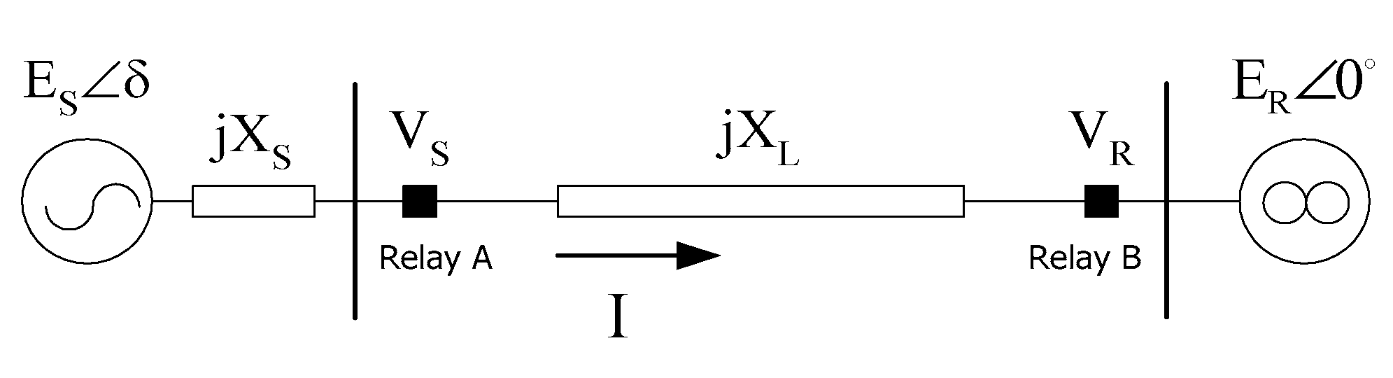
OMIB is shown in
Figure 2, in which E
S∠δ is a source (generator) voltage, E
R∠δ is a voltage of the infinite bus, Vs and V
R are voltages which are measured at the relay A and B, respectively, and jX
S and jX
L are the source and line impedances, respectively.
In
Figure 2, the voltage at relay A can be written as follows:
Equation (2) can be arranged as follows:
Now, the current at relay A can be written as:
Equation (4) may be written in conjugate form as:
A complex power S is defined as:
Substituting (3) and (5) into (6) results in:
The second term in the numerator in (7) can be rewritten as:
Similarly, the third term in the numerator in (7) can be rewritten as:
The active power is the real part of (7):
The active power in (10) can be rearranged:
where
The reactive power in (11) is:
where
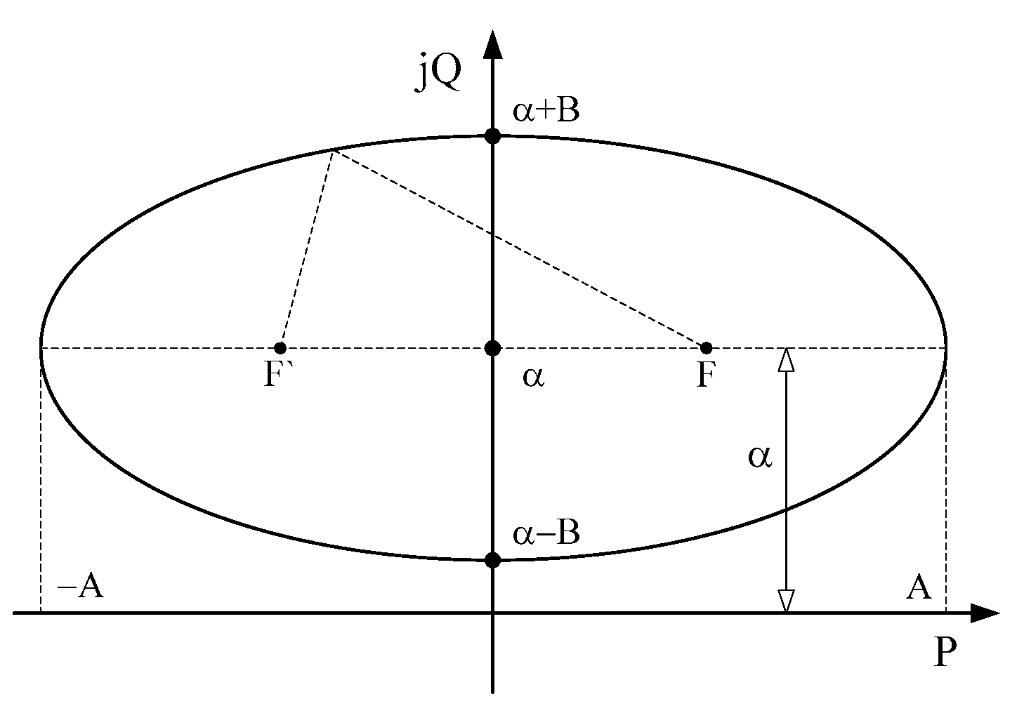
The active power in (12) and the reactive power in (14) are linked:
Equation (17) shows that the trajectory of the complex power has the shape of an ellipse and is depicted in a complex plane, as in
Figure 3 [
9,
10]. The ellipse in
Figure 3 shifts up with α along the reactive power axis, and α is the value obtained from the transmission line parameters and voltages at both sides, as shown in (16).
3. Trajectory of Complex Power
3.1. Relationship between the Generator Angle and Complex Power
In (12) and (14), the trajectory of the complex power in the complex power plane has the shape of an ellipse. When the generator angle δ is changed, the trajectory of the complex power is moved along the ellipse.
Figure 4a shows the trajectory of the complex power in the complex power plane, and
Figure 4b shows the power-angle curve. When a power swing is caused by a disturbance, the trajectory of the complex power is changed from I to IV, as shown in
Figure 4a (I→II→III→IV), and the generator angle transitions from point 1 to 5 (δ
0→ δ
1→ δ
2→ δ
1→ δ
0), as shown in
Figure 4b. The above examples suggest that the variation of the complex power in
Figure 4a and the variation of the generator angle in
Figure 4b are similar. Therefore, at the power swing condition, the variation of the reactive power Q can be used instead of the variation of the generator angle δ. The active power P and the mechanical power P
M in
Figure 4a equal to those shown in
Figure 4b.
Herein, P
M can be used to determine SEP and UEP. As shown in (12) and (14), generator angle δ, active power P, and reactive power Q have a linear relationship P = Asinδ and Q = Bcosδ + α, respectively. The relationships between δ, P, and Q are shown in
Table 1, where the active power P is 0, A is 0, and the reactive power Q is B + α, α and –B + α for the generator angle δ of 0°, 90°, and 180°, respectively.
In
Table 1, the power–angle curve can be estimated using the trajectory of the complex power.
In (12), the active power is A
.sinδ, where A is always non-negative; therefore, the active power is also non-negative when the generator angle δ changes from 0° to 180°, as shown in
Figure 5.
On the other hand, the reactive power Q and generator angle δ are related as Q = B
.cosδ + α, as shown in (14), where B can be either positive or negative. When B is positive, the reactive power Q decreases from B + α to −B + α as the generator angle δ increases from 0° to 180°, as shown in
Figure 6a. In this case, the reactive power is inversely proportional to the generator angle. However, when B is negative, the reactive power is proportional to the generator angle. From 0° to 180°, the reactive power changes along the cosine curve, as shown in
Figure 6b. When the generator angle is larger than 180°, the generator angle is increased as the reactive power is decreased. Therefore, it can be used within the generator angle range of 0° to 180°.
3.2. Time Dependency of Complex Power with Respect to the Line Parameters
Constants A and B (Equations (12) and (14)) are determined when the line parameters and the voltages at both ends of the line are known. As previously mentioned, A is always non-negative, while the sign of B is not restricted.
Figure 7 shows the trajectory of the complex power as a function of the line parameters when generator angle δ is increasing. The difference between
Figure 7a,b is in the direction of the trajectory of the complex power dependent on the sign of B, written as follows:
B from (18) is determined from the line parameters, and can be positive, negative, or zero. When B in (18) is zero, (18) becomes:
This can be rearranged as:
When the magnitude of the source impedance equals that of the line impedance, B becomes zero. When B is positive, the trajectory of the complex power is shown in
Figure 7a, where the complex power moves in the downward direction. When B is negative, the trajectory of the complex power is shown in
Figure 7b, where the complex power moves in the upward direction. When B is zero, the reactive power is α.
By using this mathematical model of complex power, a novel algorithm can be developed for estimating using complex power, instead of EAC. In brief, the trajectory of complex power can be divided into quadrants by the time variation of complex power. If the time-varying trajectory of complex power is in the first and fourth quadrants, this suggests a stable state. The 2nd and 3rd quadrants suggest an unstable state. Further details on this are given in Section 3.3 of Part II of this paper [
11].
4. Simulation Results
4.1. Simulation Method
A set of simulation tests were carried using a test model that was similar to the real system of KOREA, as shown in
Figure 8, which was interfaced with the model of a relay implemented using the ATP/EMTP MODELS [
12]. This simulation was performed to analyze the actual trajectory of the complex power system model. The transmission system modeled had a total line length of 100 km; the nominal power frequency was 60 Hz.
A simulation was carried out with a three-phase fault in the middle of one of the lines, causing the out-of-step condition. The test was repeated with various fault clearing times. The initial value of the generator angle was 30°. The simulation system was a reduced version of the actual power system, and the fault condition and operating conditions were selected in consideration of the real power system in Korea. A Synchronous Machine (SM) card and Transient Analysis on Control Systems (TACS) in EMTP were utilized, along with the parameters of the governor and excitation system of the “A” nuclear power plant in Korea [
12,
13,
14,
15].
4.2. Three Phase Fault: Clearing Time After One Cycle
When the fault clearing time is one cycle, the trajectory of the complex power is as shown in
Figure 9. After the occurrence of a three-phase fault, the generator angle increases to 89.029° and remains in a stable condition.
Figure 10 shows that the variation of the generator angle and the reactive power after the fault. Herein, the variations between them are similar. Case 4.2 is the threshold situation for OOS in the KOREA system. It shows the stable power swing. If the system has taken action, such as tripping of transmission lines and switching of the buses, there is a possibility that it will return to the stable state. However, if the fault clearing time becomes longer, the out-of-step condition will occur. To prevent the out-of-step condition, the trajectory must remain a stable power swing.
4.3. Three Phase Fault: Clearing Time After 10 Cycles
When the fault clearing time is 10 cycles, the elliptic trajectory of the complex power is as shown in
Figure 11. The time difference is only nine cycles between Case 4.2 and Case 4.3. Upon the inception of a three-phase fault, the generator angle grows beyond 90°.
Figure 12 shows the variation of the generator angle and the reactive power after the fault. During the first 7.5 s, the two trajectories are similar. At 7.5 s, the out-of-step condition of the generator begins to develop. From the results of this simulation, the variation of reactive power can be used instead of the generator angle to detect the out-of-step condition. In other words, it shows that the out-of-step state can be detected by monitoring the reactive power trajectory, and this can be used in the estimation of the stability of the power system.
4.4. Three Phase Fault: Clearing Time After 15 Cycles
To assess the performance of the presented mathematical model in a fast power swing, another simulation was performed. Case 4.4 is the totally out-of-step condition.
Figure 13 shows the trajectory of complex power. As mentioned in
Section 3 above, in
Figure 13, if the out-of-step condition is severe and fast, the trajectory of complex power has a shape of a complete ellipse. After the occurrence of a three-phase fault, the generator angle increases beyond 180°.
Figure 14 shows the variation of the generator angle and reactive power after the fault occurs. Up to about 5 s, the trajectories are similar. However, at 7.5 s, the out-of-step condition of the generator occurs. The trajectory of the complex power is close to an ellipse, and the presented mathematical model of complex power strongly suggests a possibility of application in the detection of out-of-step conditions.
The experiments on the same power system model have been carried out for various line lengths and fault locations. The obtained results were always similar to those presented in this paper.
5. Conclusions
This paper presents a rationale to analyze the trajectory of complex power in a single machine–infinite bus power system, and simulated it using ATP/EMTP MODELS. The simulation results show that the generator angle can be estimated by using the trajectory of complex power. Before the occurrence of out-of-step conditions, the time variations of complex power and the generator angle are similar, suggesting that reactive power could be used to identify the out-of-step condition. This paper shows that, for the equal area criterion, the trajectory of complex power depicts the same curve, which has the shape of an ellipse.
The trajectory of complex power is proposed as an alternative to the use of the equal area criterion for estimation of stability of a simple power system model. The proposed model uses reactive power to estimate the stability and generator angle in the power swing condition. In other words, instead of using the generator angle, the trajectory of time-varying reactive power can be used to detect and estimate the out-of-step condition more practically. In the Part II paper [
11], a detailed out-of-step detection algorithm is presented, based on the mathematical theory of the complex power trajectory presented in this paper.
In conclusion, based on the proposed theoretical basis, the out-of-step condition can be estimated and the stability of Micro Grid/Smart Grid power systems examined through the complex power trajectory, without adding new equipment installation costs.
Author Contributions
Conceptualization, methodology, C.-H.K.; simulation, writing—draft, O.-S.K., J.-Y.H.; validation, writing—review and editing, Y.-J.L. All authors have read and agreed to the published version of the manuscript.
Funding
This research was funded by the National Research Foundation of Korea (NRF) grant funded by the Korea government (MSIP), grant number No. 2018R1A2A1A05078680.
Conflicts of Interest
The authors declare no conflict of interest.
References
- Jonsson, M.; Daalder, J.E. An adaptive scheme to prevent undesirable distance protection operation during voltage instability. IEEE Trans. Power Deliv. 2003, 18, 1174–1180. [Google Scholar] [CrossRef]
- Machowski, J.; Bialek, J.; Bumby, J.R. Power System Dynamics and Stability; John Wiley & Sons Inc.: Hoboken, NJ, USA, 1998; pp. 215–234. [Google Scholar]
- Bollen, M.H.J. Understanding Power Quality Problems; Wiley-IEEE Press: Hoboken, NJ, USA, 2000; pp. 319–321. [Google Scholar]
- Stevenson, W.D. Elements of Power System Analysis; McGraw-Hill: New York, NY, USA, 1982; pp. 393–400. [Google Scholar]
- Anderson, P.M. Power System Protection; Wiley-IEEE Press: Hoboken, NJ, USA, 1998; pp. 853–905. [Google Scholar]
- Xue, Y.; Van Custem, T.; Ribbens-Pavella, M. Extended equal area criterion justifications, generalizations, applications. IEEE Trans. Power Syst. 1989, 4, 44–52. [Google Scholar] [CrossRef]
- Xue, Y.; Wehenkel, L.; Belhomme, R.; Rousseaux, P.; Pavella, M.; Euxibie, E.; Heilbroon, B.; Lesigne, J.-F. Extended equal area criterion revisited. IEEE Trans. Power Syst. 1992, 7, 1012–1022. [Google Scholar] [CrossRef]
- Li, Y.-Q.; He, T.; Liu, W.-S.; Liu, J.-F. The study on real-time transient stability emergency control in power system. In Proceedings of the 2002 IEEE Canadian Conference on Electrical & Computer Engineering, Winnipeg, MB, Canada, 12–15 May 2002; pp. 134–143. [Google Scholar]
- Lockwood, E.H. A Book of Curves; Cambridge University Press: Cambridge, UK, 1967; pp. 13–24. [Google Scholar]
- Yates, R.C. A Handbook on Curves and Their Properties; J.W. Edwards: Ann Arbor, MI, USA, 1952; pp. 36–56. [Google Scholar]
- Lee, Y.J.; Kwon, O.S.; Heo, J.Y.; Kim, C.H. A Study on the Out-of-Step Detection Algorithm Using Time Variation of Complex Power—Part II: Out-of-Step Detection Algorithm and Simulation Results. Energies 2020, 13, 1833. [Google Scholar] [CrossRef]
- Kim, C.H.; Lee, M.H.; Aggarwal, R.K.; Johns, A.T. Educational use of EMTP MODELS for the study of a distance relaying algorithm for protecting transmission lines. IEEE Trans. Power Syst. 2000, 15, 9–15. [Google Scholar]
- Ahn, S.P.; Kim, C.H.; Aggarwal, R.K.; Johns, A.T. An alternative approach to adaptive single pole auto-reclosing in high voltage transmission systems based on variable dead time control. IEEE Tran. Power Deliv. 2001, 16, 676–686. [Google Scholar] [CrossRef]
- Jang, S.I.; Shin, M.C.; Yoon, C.D.; Campbell, R.C. A study on adaptive autoreclosure scheme with real-time transient stability. J. Electr. Eng. Technol. 2006, 1, 8–15. [Google Scholar] [CrossRef]
- Kim, C.H.; Heo, J.Y.; Aggarwal, R.K. An enhanced zone 3 algorithm of a distance relay using transient components and state diagram. IEEE Trans. Power Deliv. 2005, 20, 39–46. [Google Scholar]
© 2020 by the authors. Licensee MDPI, Basel, Switzerland. This article is an open access article distributed under the terms and conditions of the Creative Commons Attribution (CC BY) license (http://creativecommons.org/licenses/by/4.0/).


