Research on D-STATCOM Double Closed-Loop Control Method Based on Improved First-Order Linear Active Disturbance Rejection Technology

Abstract

The application of a distribution static synchronous compensator (D-STATCOM) is the best technical means to solve the problem of reactive power compensation and harmonics. The D-STATCOM system has the characteristics of variable parameters, strong coupling, nonlinearity and multi-variability. In order to improve the speed of the dynamic tracking response and anti-disturbance capability of the D-STATCOM, the article proposes an improved Linear Active Disturbance Rejection Controller (LADRC) based on the total disturbance deviation control method. Combined with double closed-loop control, the inner loop takes the current as the state variable, and the outer loop uses the DC side output voltage as the state variable to achieve robust stability of the D-STATCOM and controller output. The simulation results show that the improved LADRC is more stable than the traditional LADRC in controlling the DC voltage waveform of the compensator, reactive current tracking and reactive power compensation waveform when it is disturbed, which verifies the superiority and feasibility of the improved LADRC.

1. Introduction

A distribution static synchronous compensator (D-STATCOM) is a kind of parallel device for reactive power compensation, which is mainly used in low-voltage distribution networks [1]. It has the characteristics of powerful functions, excellent performance and high cost performance. Various static reactive power compensators and their control strategies are constantly improving. The control strategies proposed by experts at home and abroad are generally divided into three categories: (1) Traditional proportional integral control [2], (2) intelligent control technologies such as neural networks and sliding mode control [3,4,5] and (3) control methods based on traditional modern control theory [6]. All kinds of control methods have certain limitations. Traditional PI (Proportional-Integral) control cannot solve the problem of the system remaining stable when it is disturbed by uncertainty. When faced with some nonlinear, time-varying, coupling and uncertain parameters and structure, the control effect is not particularly ideal, and in this case, the controller is no longer suitable. The convergence speed of an intelligent control algorithm is slow and it cannot reach the requirement of expected real-time control. The accuracy of the dynamic model of the controller is the key to the control effect. For complex systems, it is often difficult to accurately describe the dynamic characteristics of the system due to a large amount of control. However, the state space expression depends on the precise mathematical model of the system. For D-STATCOM, which is composed of IGBT (Insulated Gate Bipolar Translator) components, the internal harmonic content of the system is ignored during the precise modeling. The mathematical model of modern control theory based on state-space theory adopts the state-space equation, which mainly focuses on time domain analysis. The state equation can only describe a stable system, focusing on the system state and its internal relations. Therefore, the modern control theory cannot achieve a satisfactory control effect in the practical system.

The technology of the Active Disturbance Rejection Controller (ADRC) was proposed by Han J.Q. researchers in the process of deeply studying the inherent essence of traditional PID (Proportion Integration Differentiation) controllers [7]. It provides a new idea for disturbance compensation, and its core element is an extended state observer (ESO), using a state observer to establish a modified model of the controlled object, innovatively putting forward a new state variable, taking the internal and external disturbances as the total disturbance and using the observer to observe [8]. Based on that, Professor Gao Z.Q. proposed the Linear Active Disturbance Rejection Controller. Through the pole assignment in the frequency domain, the parameters to be set are reduced to three, which greatly simplifies the controller parameter tuning. Reference [9] simplified the structure of a nonlinear ADRC and proposed an LADRC method.

The technology of the Linear Active Disturbance Rejection Controller has been applied in many advanced fields of science and technology, such as missile weapons, precision control [10], etc., but although it has great engineering application value, LADRC is rarely used in D-STATCOM systems. Reference [11] applied nonlinear ADRC control to the inner current loop of a D-STATCOM. However, the controller has complicated parameter adjustment and lacks proof of controller stability. Reference [12] proposed an improved LADRC strategy and method, but it has not been applied to actual physical systems.

In this paper, the improved Linear Active Disturbance Rejection technology is implemented to control the D-STATCOM system and the proposed control strategy is simulated and analyzed. Firstly, the mathematical model of the D-STATCOM in a two-phase rotating coordinate system is achieved by coordinate transformation [13]. Then the traditional LADRC is improved and applied to the current and voltage loops of the system. The disturbance rejection ability and convergence of LESO, as well as the stability and disturbance rejection characteristics of the LADRC combined with the system are analyzed by using classical control theory. Finally, the control performance of the improved LADRC and the traditional LADRC is compared and analyzed by MATLAB/Simulink simulation.

In this article, the second part introduces the mathematical model of the D-STATCOM, and then in the third part, the methods of improving the LADRC are proposed by deeply studying the connotations of the traditional first-order LADRC and second-order LESO. Combining the LADRC control with the D-STATCOM system, the improved LADRC is applied to the D-STATCOM voltage and current double loop, and the corresponding controller is designed. The fourth part proves the improvement of LESO’s anti-interference characteristics and convergence in the frequency domain. As well as the anti-disturbance characteristics of the improved LADRC combined with the actual D-STATCOM system, the Lynard–Chiapart principle is used to prove the stability of the controller. In the fifth part, the simulation results prove the superiority and feasibility of the improved LADRC compared with the traditional LADRC.

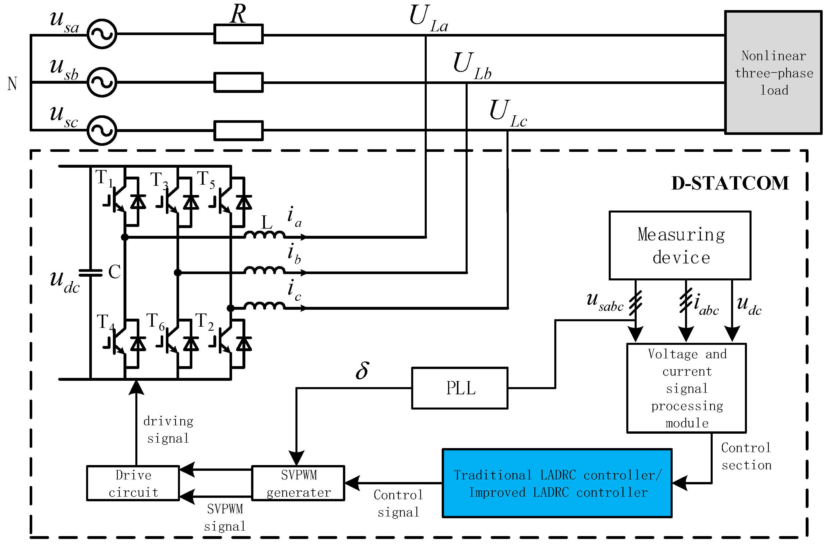
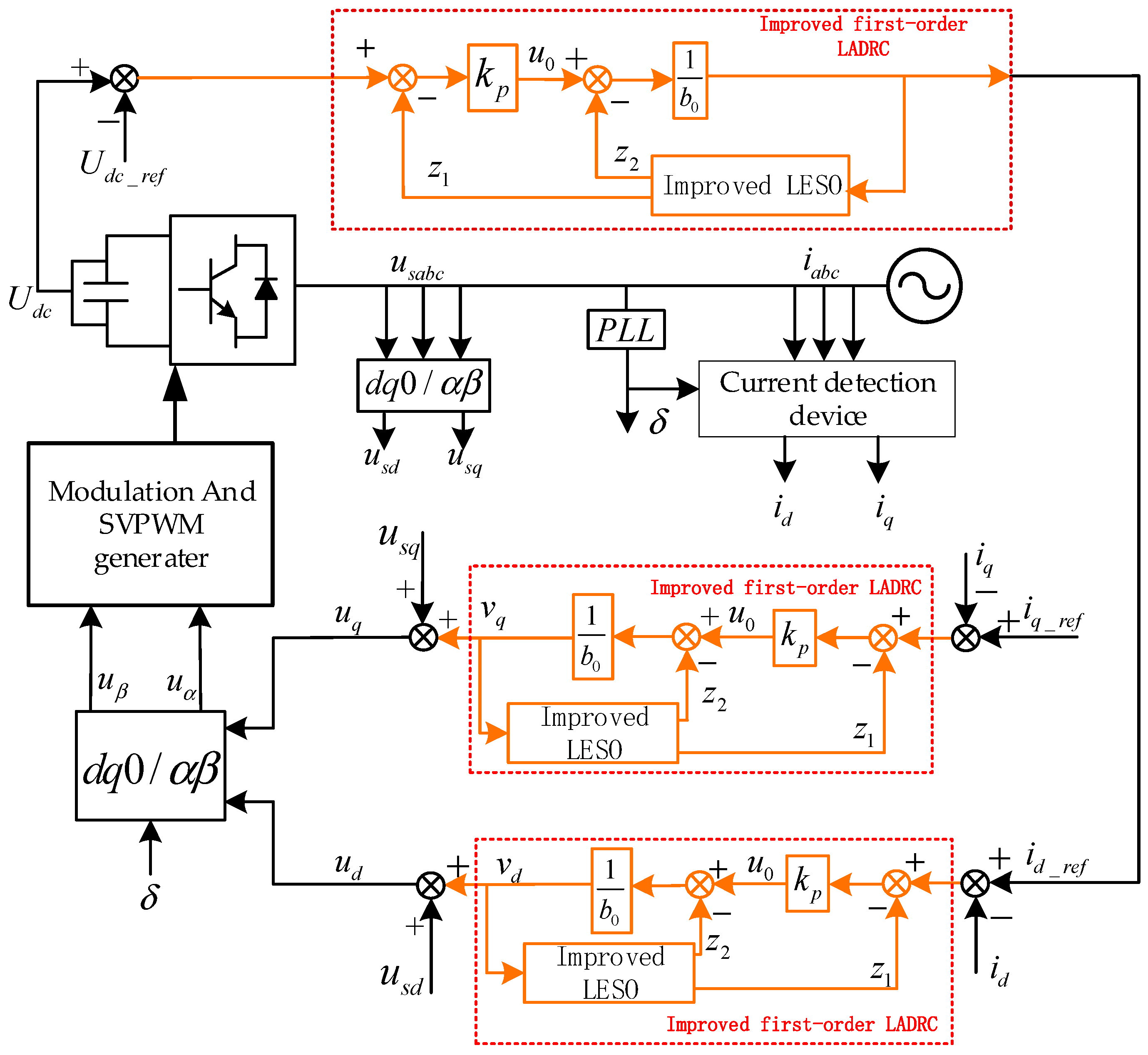
2. Mathematical Modeling of the D-STATCOM System

The typical structure of the D-STATCOM system is shown in Figure 1, where $u_{sa}$, $u_{sb}$, $u_{sc}$ are representative of the three-phase grid voltage; $R$ is the line resistance at the grid side; $L$ is the filter inductance between the D-STATCOM and the grid connection point; $C$ is the capacitance at the DC side; $u_{dc}$ is representative of the voltage of the DC side; $i_a$, $i_b$, $i_c$ are the actual output currents of the compensator; $U_{La}$, $U_{Lb}$, $U_{Lc}$ are the measured voltages at the output of the D-STATCOM. The control structure of the STATCOM consists of two parts, one is the drive circuit space vector pulse width modulation (SVPWM), the other is the control layer. $u_{sabc}$ depicts the three-phase voltage at the D-STATCOM side and output side and $i_{abc}$ is the three-phase current output [14].

The compensation coefficient of the D-STATCOM is 1 and the output harmonic content of the device is ignored. Then, according to Kirchhoff’s voltage law, the mathematical model of the D-STATCOM in a static three-phase coordinate system is as follows [15]:

$$\{\begin{array}{l}L\frac{d{i}_a}{dt}=U_{La}-u_{sa}-R{i}_a\\ L\frac{d{i}_b}{dt}=U_{Lb}-u_{sb}-R{i}_b\\ L\frac{d{i}_c}{dt}=U_{Lc}-u_{sc}-R{i}_c\\ C\frac{d{u}_{dc}}{dt}=-i_a\sin \left(\omega t-\delta \right)-\\ \hspace{1em}\hspace{1em}\hspace{1em}\hspace{1em}\hspace{1em}{i}_b\sin \left(\omega t-\frac{2}{3}\pi -\delta \right)-i_c\sin \left(\omega t+\frac{2}{3}\pi -\delta \right)\end{array}$$

(1)

Among them:

$$\{\begin{array}{l}{U}_{La}=u_{dc}\sin (\omega t-\delta )\\ U_{Lb}=u_{dc}\sin (\omega t-\frac{2}{3}\pi -\delta )\\ U_{Lc}=u_{dc}\sin (\omega t+\frac{2}{3}\pi -\delta )\end{array}$$

(2)

It can be seen from Equation (1) that the design of the controller is complex because the three-phase current is time-varying. Therefore, the coordinate transformation method is used to transform the mathematical model in the three-phase static coordinate system into the two-phase synchronous rotating coordinate system. The transformation matrix is as follows:

$$P=\frac{2}{3}\left[\begin{array}{ccc}\cos \theta & \cos \left(\theta -2\pi /3\right)& \cos \left(\theta +2\pi /3\right)\\ -\sin \theta & -\sin \left(\theta -2\pi /3\right)& -\sin \left(\theta +2\pi /3\right)\\ \sqrt{2}/2& \sqrt{2}/2& \sqrt{2}/2\end{array}\right]$$

(3)

Equation (1) through coordinate transformation. The D-STATCOM is obtained at dq0. The mathematical model in a rotating coordinate system [16]:

$$\{\begin{array}{l}L\frac{d{i}_d}{dt}=\omega L{i}_q-R{i}_d-u_{sd}+U_{Ld}\\ L\frac{d{i}_q}{dt}=-\omega L{i}_d-R{i}_q-u_{sq}+U_{Lq}\end{array}$$

(4)

$$C\frac{d{u}_{dc}}{dt}=\sqrt{\frac{3}{2}}\left(\cos \delta i_d+\sin \delta i_q\right)$$

(5)

In Equations (4) and (5), $u_{sd}$ and $u_{sq}$ are the voltage components of the d-axis and q-axis on the grid side after coordinate transformation; $U_{Ld}$ and $U_{Lq}$ are the voltage components of the D-STATCOM system output voltage; $i_d$ and $i_q$ are the d-axis and q-axis components of the D-STATCOM injection grid side current, respectively. The $\delta$ between the grid voltage and the output voltage of the static var compensator can be used to determine whether the system absorbs or emits reactive power.

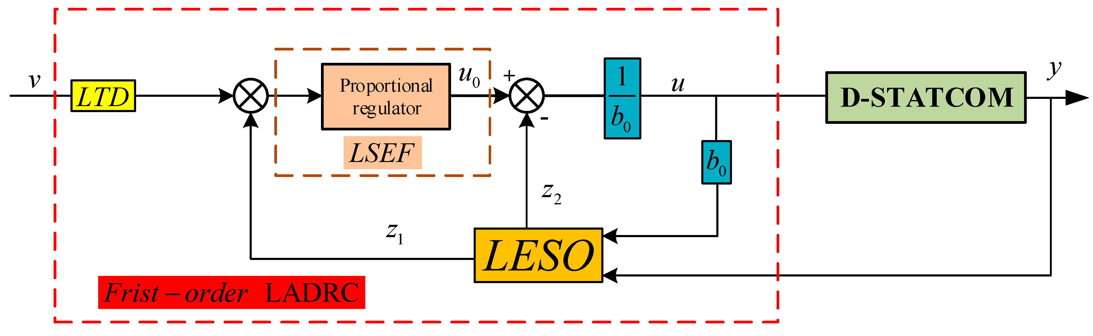
3. Principle Analysis of Traditional LADR and Improved LADRC Structure Design

The LADRC consists of Linear State Error Feedback (LSEF), a Linear Extend State Observer (LESO) and a Linear Tracking Differentiator (LTD) [17]. The LTD introduces a differential into the controller to avoid the contradiction between overshoot and rapidity. It is the core of LADRC that the total disturbance of the LESO observation system is estimated and compensated in real time. LSEF synthesizes the interference estimation to create control signals. The traditional structure of the LADRC is shown in Figure 2.

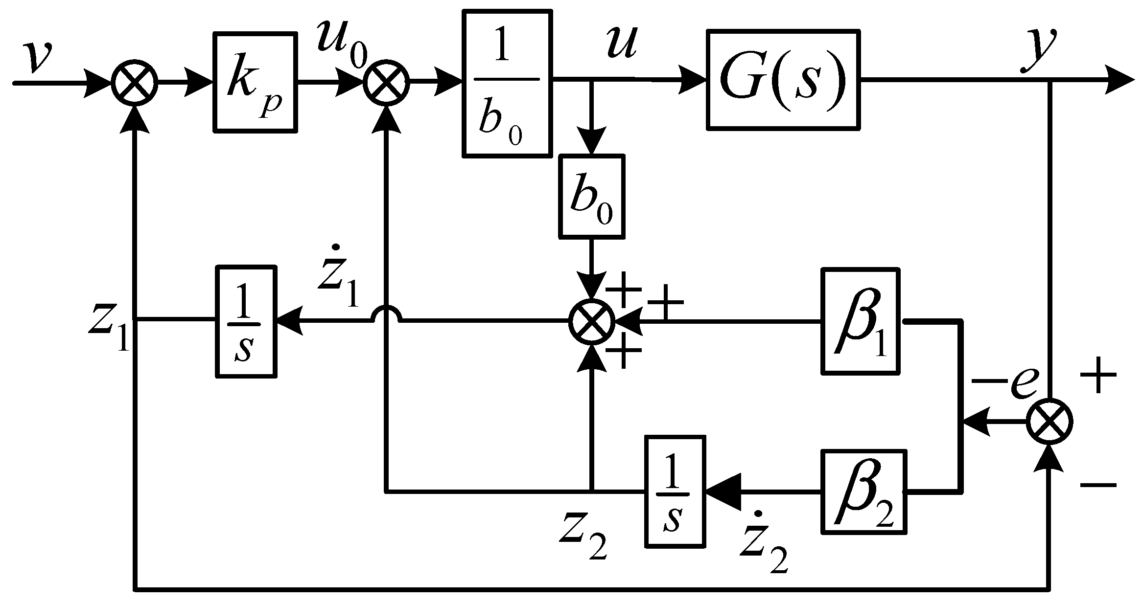
3.1. Design of Traditional LADRC

It can be seen from Equation (4) that there are two first-order differential equations, and the two-state variables are coupled to each other, which can be regarded as a defined generalized disturbance of the controlled object, to achieve the purpose of decoupling. Because LADRC does not need to rely on a specific mathematical model of the controlled object, the differential equation of the controlled object can be written in the following general form:

$$\dot{y}=-a_{0}y+bu+w$$

(6)

where $w$ is an unknown external disturbance and $b$ is the input control gain. Since $b_0$ is known, this equation can be written as:

$$\dot{y}=-a_{0}y+\left(b-b_0\right)u+b_{0}u+w$$

(7)

where $-a_{0}y+(b-b_0)u+w$ is the sum of the total unknown disturbance and the information of the known object, recorded as $f$. $x_1=y$ and $x_2=f$ are selected as state variables. The transformation into a continuous state is described as follows:

$$\{\begin{array}{l}\dot{x}=Ax+Bu+E\dot{f}\\ y=Cx\end{array}$$

(8)

Among them: $A=\left[\begin{array}{cc}0& 1\\ 0& 0\end{array}\right]$, $B=\left[\begin{array}{c}{b}_0\\ 0\end{array}\right]$, $E=\left[\begin{array}{c}0\\ 1\end{array}\right]$, $C=\left[\begin{array}{cc}1& 0\end{array}\right]$. The corresponding LESO is established as follows:

$$\{\begin{array}{l}e=z_1-x_1\\ {\dot{z}}_1=z_2-{\beta }_{1}e+b_{0}u\\ {\dot{z}}_2=-{\beta }_{2}e\end{array}$$

(9)

In Equation (9), $z_1$ and $z_2$ are state variables of the linear extended state observer, and the state variable $z_1$ tracks the output $y$ of the system and $z_2$ tracks total disturbance $f$. By selecting the appropriate observer gain coefficients ${\beta }_1$ and ${\beta }_2$, the observer state variables can be used to observe the system output $y$ and the total disturbance $f$.

Design of the system disturbance compensation link:

$$u=\frac{-z_2+u_0}{b_0}$$

(10)

If the estimation error of the observer is ignored, Equation (8) can be simplified as:

$$\dot{y}=x_2+b_{0}u=x_2+\left(-z_2+u_0\right)\approx u_0$$

(11)

The response rate of the construction error:

$$u_0=k_p\left(v-z_1\right)$$

(12)

$v$ is the given reference input and $k_p$ is the proportional control coefficient. The closed-loop transfer function of the controller is:

$$G\left(s\right)=\frac{k_p}{s+k_p}$$

(13)

Let the controller bandwidth $k_p={\omega }_c$ and configure observer poles at $-{\omega }_0$ [18]. For Equation (8), it can be obtained:

$$\lambda \left(s\right)=s^2+{\beta }_{1}s+{\beta }_2={\left(s+{\omega }_0\right)}^2$$

(14)

where ${\omega }_0$ is the observer bandwidth, and the bandwidth gain obtained is:

$$\left[\begin{array}{c}{\beta }_1\\ {\beta }_2\end{array}\right]=\left[\begin{array}{c}2{\omega }_0\\ {\omega }_0^2\end{array}\right]$$

(15)

At this point, the selection of $b_0$, ${\omega }_0$ and ${\omega }_c$ will affect the control performance of the traditional LADRC. Equations (9), (10) and (12) constitute the structure block diagram of the traditional LADRC, as shown in Figure 3.

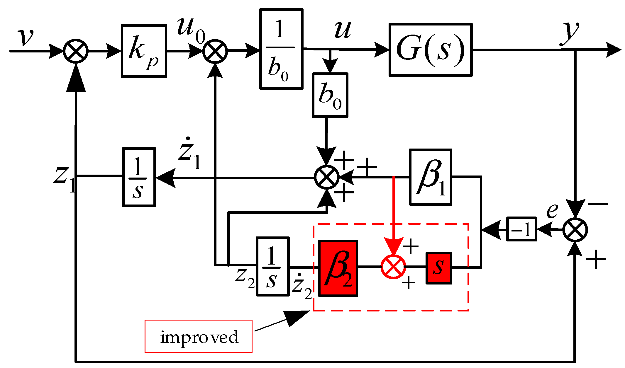
3.2. Design of Improved LADRC

The traditional LADRC controls the D-STATCOM by using the deviation between the given value and the actual feedback value and makes the deviation close to zero to achieve the control purpose. The key is that the LESO can observe the total disturbance from inside and outside the system and compensate the controlled quantity according to the observation disturbance in real time. Taking the d-axis of the D-STATCOM as an example, the controlled system is a first-order linear differential equation, so the first-order LADRC is selected for improved analysis. For the traditional LESO corresponding to the first-order system, refer to Equation (9).

It can be seen from the formula that the adjustment of $z_1$ and $z_2$ is achieved through the deviation of $e_1$, so that it can track the actual value of the state variable needed. In order to get a better control effect in the traditional LESO it is important to make the $z_1$ approach $x_1$, which makes $e_1$ approach zero quickly. Secondly, $z_2$ approaches $x_2$. Once the order is disordered, the control function of the controller fails. If $z_1$ has tracked $x_1$, that is, $e_1$ has approached zero, then it becomes difficult to control $z_2$ in order. Because of this, the traditional LESO can only select a larger observer bandwidth to weaken the feature that the deviation of $e_1$ is small. To solve this contradiction, this paper proposes to redefine the deviation quantity of control $z_2$ [19]. The traditional LESO is rewritten as:

$$\{\begin{array}{l}{z}_1=e_1+x_1\\ z_2={\dot{z}}_1+{\beta }_1{e}_1-b_{0}u\end{array}$$

(16)

From Equations (9) and (16), it can be obtained that:

$$\{\begin{array}{c}{z}_1=x_1+e_1\\ z_2=x_2+{\dot{e}}_1+{\beta }_1{e}_1\end{array}$$

(17)

It can be concluded that the deviation of control $z_2$ and $x_2$ becomes ${\dot{e}}_1+{\beta }_1{e}_1$. During the operation of the LESO, each state variable and its derivative is continuously differentiable, so the derivatives of $e_1$ can be calculated. Therefore, this deviation is regarded as a new change rate of $z_2$, and then an improved LESO can be obtained:

$$\{\begin{array}{c}{e}_1=z_1-x_1\\ {\dot{z}}_1=z_2-{\beta }_1{e}_1+b_{0}u\\ {\dot{z}}_2=-{\beta }_2\left({\dot{e}}_1+{\beta }_1{e}_1\right)\end{array}$$

(18)

The poles of the improved LADRC observer are reconfigured and also configured to $-{\omega }_0$. The observer matrix is rewritten:

$$\left(\begin{array}{c}{\dot{z}}_1\\ {\dot{z}}_2\end{array}\right)=\left(\begin{array}{cc}-{\beta }_1& 1\\ 0& -{\beta }_2\end{array}\right)\left(\begin{array}{c}{z}_1\\ z_2\end{array}\right)+\left(\begin{array}{ccc}{b}_0& {\beta }_1& 0\\ -b_0{\beta }_2& 0& {\beta }_2\end{array}\right)\left(\begin{array}{c}u\\ y\\ \dot{y}\end{array}\right)$$

(19)

Then $\dot{y}$ is the derivative of the output variable $y$. The observer characteristic equation is:

$${\lambda }_1\left(s\right)=\left(s+{\beta }_1\right)\left(s+{\beta }_2\right)={\left(s+{\omega }_0\right)}^2$$

(20)

Therefore:

$$\left[\begin{array}{c}{\beta }_1\\ {\beta }_2\end{array}\right]=\left[\begin{array}{c}{\omega }_0\\ {\omega }_0\end{array}\right]$$

(21)

At this time, the overall structure control block diagram of the improved LADRC is as follows Figure 4:

At this point, the mathematical model of the improved LADRC is:

$$\{\begin{array}{c}{\dot{z}}_1=z_2+b{u}_0-{\beta }_1\left(z_1-y\right)\\ \begin{array}{l}{\dot{z}}_2=-{\beta }_2\left[\left({\dot{z}}_1-\dot{y}\right)+{\beta }_1\left(z_1-y\right)\right]\\ \hspace{1em}\hspace{1em}\hspace{1em}{u}_0=k_p\left(v-z_1\right)\\ \hspace{1em}\hspace{1em}\hspace{1em}\hspace{1em}\hspace{1em}u=\frac{u_0-z_2}{b_0}\end{array}\end{array}$$

(22)

3.3. Design of D-STATCOM Controller Based on Improved LADRC

3.3.1. Design of Current Inner Loop Controller

Taking the d-axis current as an example, it can be known from Equation (4) that:

$$\frac{d{i}_d}{dt}=\omega i_q-\frac{1}{L}R{i}_d-\frac{1}{L}{u}_{sd}+\frac{1}{L}{U}_{Ld}$$

(23)

The first-order improved LADRC is adopted to construct the state-space equation:

$$\{\begin{array}{l}{\dot{x}}_{1i}=x_{2i}+b_{0i}{u}_i\\ {\dot{x}}_{2i}={\dot{f}}_i\\ y_i=x_{1i}\end{array}$$

(24)

where $x_{1i}$ is the actual current $i_d$ of the d-axis and $x_{2i}$ is a new variable of system expansion.

$f_i=-\frac{R}{L}{i}_d+\omega i_q-\frac{1}{L}{u}_{sd}$, $b_0=\frac{1}{L}$, $u_i$ is the given current of the system $i_{d\_ref}$. Then the LADRC of the d-axis of the inner current loop is [20,21]:

$$\{\begin{array}{c}{\dot{z}}_{1i}=z_{2i}+b_{0i}{u}_i-{\beta }_1\left(z_{1i}-y\right)\\ \begin{array}{l}{\dot{z}}_{2i}=-{\beta }_2\left[\left({\dot{z}}_{1i}-\dot{y}\right)+{\beta }_1\left(z_{1i}-y\right)\right]\\ \hspace{1em}\hspace{1em}{u}_{0i}=k_p\left(i_{d\_ref}-z_{1i}\right)\\ \hspace{1em}\hspace{1em}\hspace{1em}{u}_i=\frac{u_{0i}-z_{2i}}{b_{0i}}\end{array}\end{array}$$

(25)

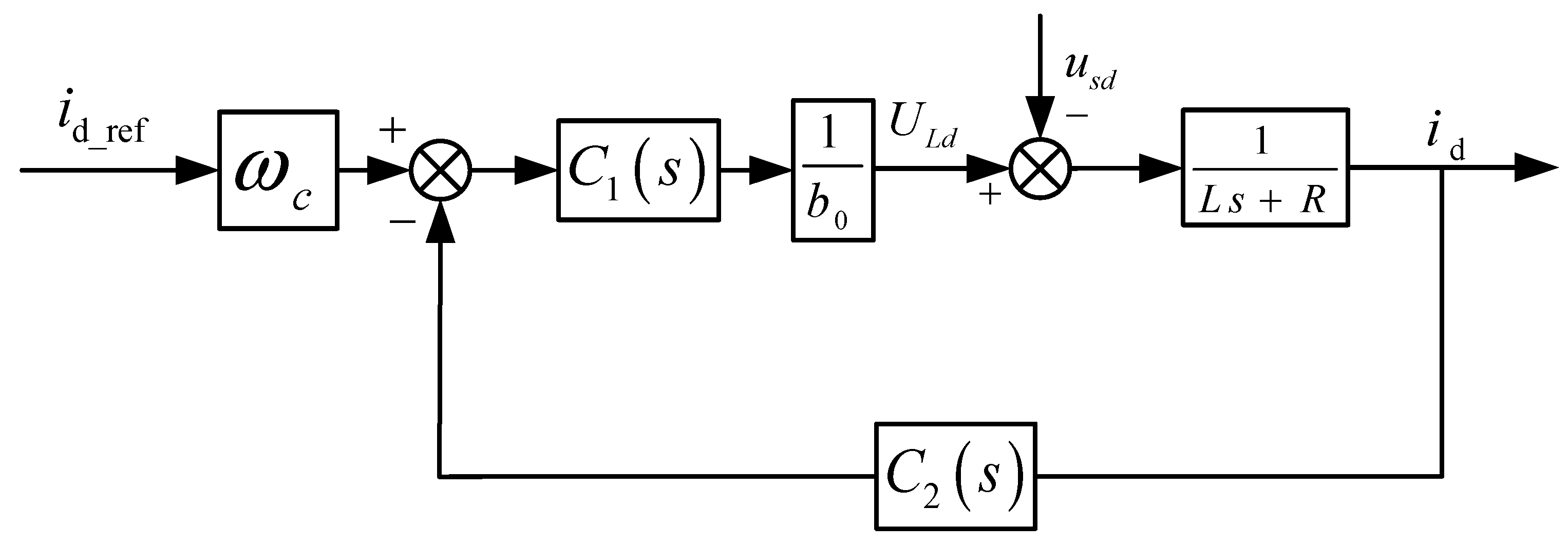
3.3.2. Design of Voltage Outer Loop Controller

From Equation (5), we can get:

$$\frac{d{u}_{dc}}{dt}=\sqrt{\frac{3}{2}}\frac{1}{C}\left(\cos \delta i_{\mathrm{d}}+\sin \delta i_{\mathrm{q}}\right)$$

(26)

The state equation of the outer voltage loop is constructed:

$$\{\begin{array}{l}{\dot{x}}_{1u}=x_{2u}+b_{0u}{u}_u\\ {\dot{x}}_{2u}={\dot{f}}_u\\ y_u=x_{1u}\end{array}$$

(27)

At this time, $x_{1u}$ is the actual output voltage on the DC side of the D-STATCOM system and $x_{2u}$ is a new variable of system expansion.$f_u=\sqrt{\frac{3}{2}}\frac{\sin \delta i_q}{C}$, $b_0=\sqrt{\frac{3}{2}}\frac{1}{C}$, $u_u=u_{dc\_ref}$. The LADRC of the outer loop is:

$$\{\begin{array}{c}{\dot{z}}_{1u}=z_{2u}+b_{0u}{u}_u-{\beta }_1\left(z_{1u}-y\right)\\ \begin{array}{l}{\dot{z}}_{2i}=-{\beta }_2\left[\left({\dot{z}}_{1u}-\dot{y}\right)+{\beta }_1\left(z_{1u}-y\right)\right]\\ \hspace{1em}\hspace{1em}\hspace{1em}{u}_{0u}=k_p\left(u_{dc\_ref}-z_{1u}\right)\\ \hspace{1em}\hspace{1em}\hspace{1em}{u}_u=\frac{u_{0u}-z_{2u}}{b_{0u}}\end{array}\end{array}$$

(28)

Now the double closed-loop LADRC for the D-STATCOM system is designed. The improved LADRC is applied to the current inner loop and the voltage outer loop. The overall structure diagram of the system is shown in Figure 5.

4. Performance Index Analysis of Improved LADRC in Frequency Domain

It can be seen from Figure 3 that the first-order LADRC is a feedback system, and its essential problem is the proof of system stability. The LESO is the core structure of Linear Active Disturbance Rejection Control technology. Its function is to estimate and compensate the total disturbance by observation. In this paper, the classical control principle is applied to analyze the immunity and convergence of the LESO, and the immunity and stability of the LADRC is combined with the actual D-STATCOM system.

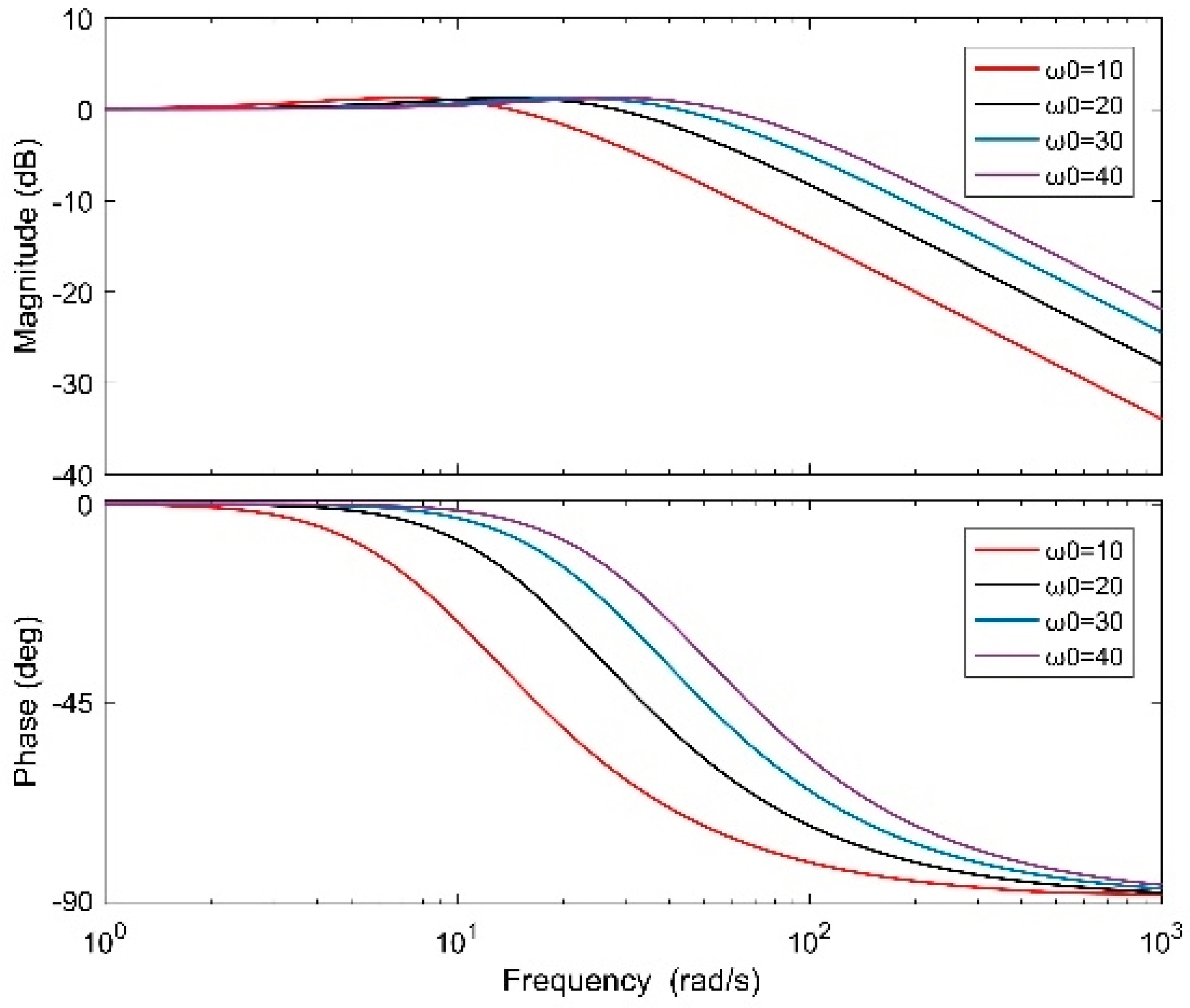
4.1. Disturbance Immunity Analysis of Improved LESO

The Laplace transform of Equation (19) can be obtained by:

$$Z_1\left(s\right)=\frac{{\omega }_0^2+2{\omega }_{0}s}{{\left(s+{\omega }_0\right)}^2}Y\left(s\right)+\frac{b_{0}s}{{\left(s+{\omega }_0\right)}^2}U\left(s\right)$$

(29)

$$Z_2\left(s\right)=\frac{{\omega }_{0}s}{s+{\omega }_0}Y\left(s\right)-\frac{b_0{\omega }_0}{s+{\omega }_0}U\left(s\right)$$

(30)

This section focuses on the effect of noise perturbation ${\eta }_c$ of output variable $y$ and control variable ${\eta }_r$ of output perturbation $u$ on the improved LESO. The transfer function of the observed noise can be obtained from Equation (29):

$$\frac{z_1}{{\eta }_c}=\frac{{\omega }_0^2+2{\omega }_{0}s}{{\left(s+{\omega }_0\right)}^2}$$

(31)

${\omega }_0=10,20,30,40$ are set, respectively, to obtain the Bode plot curve of this transfer, as shown in Figure 6:

According to its frequency domain characteristic curve, it can be concluded that with the increase in ${\omega }_0$, the system bandwidth becomes larger and the tracking speed increases accordingly.

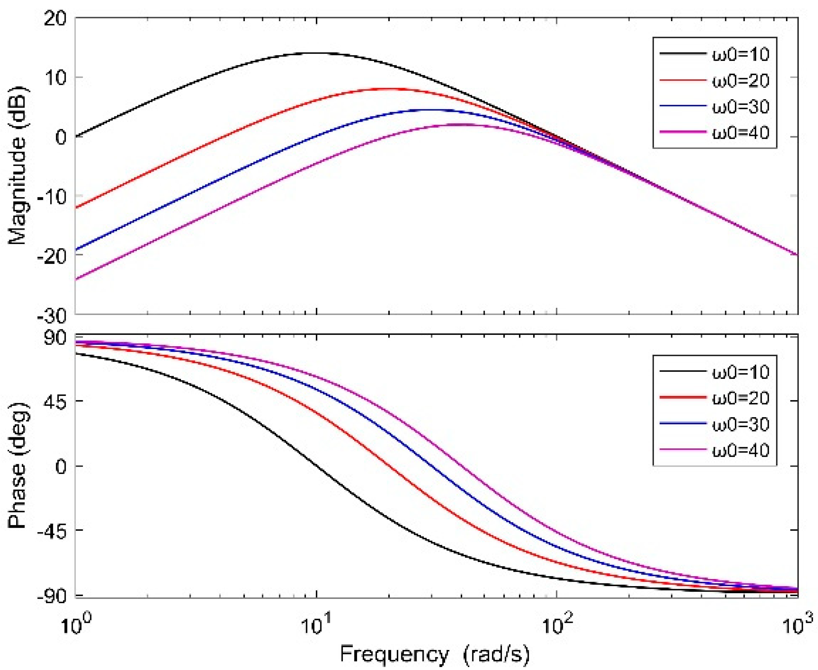
According to Equation (29), the input disturbance transfer function is as follows:

$$\frac{z_1}{{\eta }_r}=\frac{b_{0}s}{{\left(s+{\omega }_0\right)}^2}$$

(32)

$b=100$ and ${\omega }_0=10,20,30,40$ are set and the frequency domain characteristic curve of the disturbance transfer function at the input can be obtained.

It can be seen that, compared with Figure 6, with the increase in ${\omega }_0$, the disturbance phase of the tracking input in Figure 7 becomes increasingly delayed, but the high-frequency gain is almost unchanged. It can be seen that the system has a good inhibition effect on input disturbance. From the above analysis, it can be seen that the improved LESO has good disturbance resistance and strong robustness for the observed disturbance and the actual input disturbance.

4.2. Convergence and Error Estimation of Improved LESO

$E_1\left(s\right)=Z_1\left(s\right)-Y\left(s\right)$ are used in Equation (29) to get:

$$E_1\left(s\right)=-\frac{s^2}{{\left(s+{\omega }_0\right)}^2}Y\left(s\right)+\frac{b_{0}s}{{\left(s+{\omega }_0\right)}^2}U\left(s\right)$$

(33)

From $f=x_2=\dot{y}-b_{0}u$ we can get:

$$F\left(s\right)=sY\left(s\right)-b_{0}U\left(s\right)$$

(34)

In the Laplace transformation formula, $F\left(s\right)$ is $f$. In the same way, $E_2\left(s\right)=Z_2\left(s\right)-F\left(s\right)$ is used to obtain:

$$E_2\left(s\right)=-\frac{s^2}{s+{\omega }_0}Y\left(s\right)+\frac{b_{0}s}{s+{\omega }_0}U\left(s\right)$$

(35)

For the convenience of analysis, $Y\left(s\right)$ and $U\left(s\right)$ are all taken as step signals, namely: $Y\left(s\right)=U\left(s\right)=\frac{K}{s}$. The steady-state error of the system can be obtained as follows:

$$\{\begin{array}{l}{E}_{s1}\left(s\right)=\underset{s\to 0}{\lim }s{E}_1\left(s\right)=0\\ E_{s2}\left(s\right)=\underset{s\to 0}{\lim }s{E}_2\left(s\right)=0\end{array}$$

(36)

The above formula shows that the LESO has good convergence, and it can guarantee the estimation of state variables without difference and realize the disturbance rejection and compensation of the controller to the total disturbance. In the following, the transient process is analyzed in the time domain by the undetermined coefficient method. When $b_0=0$, it can be obtained:

$$Z_1\left(s\right)=K(\frac{1}{s}-\frac{1}{s+{\omega }_0}+\frac{{\omega }_0}{{\left(s+{\omega }_0\right)}^2})$$

(37)

The inverse Laplace transform of the above equation is:

$$z_1\left(t\right)=K-K\left(1-{\omega }_{0}t\right)e^{-{\omega }_{0}t}\left(t\ge 0\right)$$

(38)

The maximum value of $t_{\max }=2/{\omega }_0$ is found and used in Equation (39) to get:

$$z_1{}_{\max }=K\left(1+e^{-2}\right)\approx 1.135K$$

(39)

Since the output signal $y\left(t\right)$ is a step signal, it suddenly changes at zero time. At this time, the estimation error $e$ no longer inclines to zero, and the maximum error can reach 13.5%. However, there is a delay in the power system. Because the output of the inertial D-STATCOM does not change abruptly throughout the power network, the error of state variable estimation by this improved LESO approximates zero when time $t$ tends to infinity. Therefore, the estimation and tracking of the state variable of the improved LESO does not have serious errors.

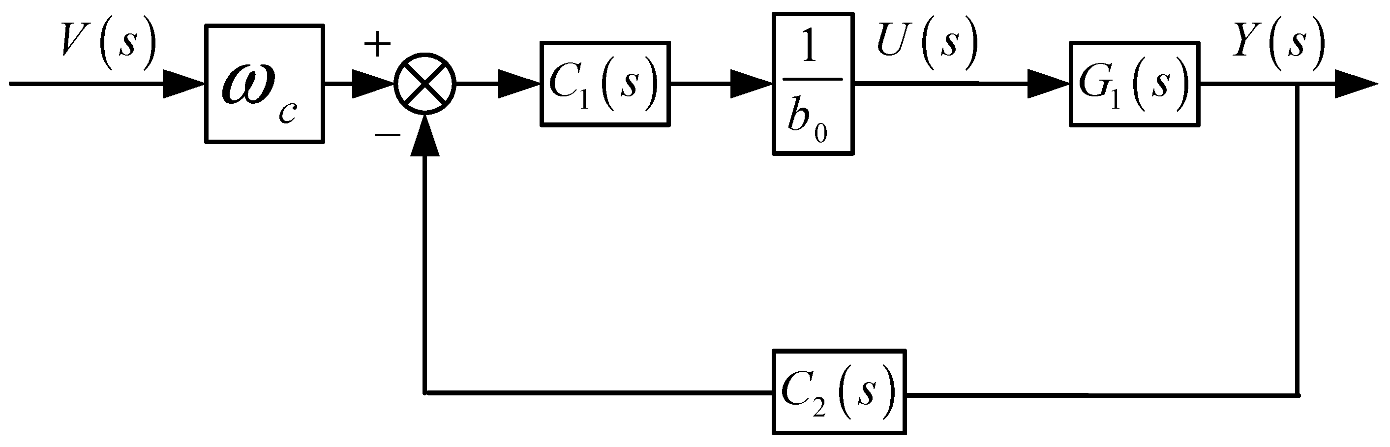
4.3. Performance Analysis of Improved LADRC Combined with D-STATCOM System

4.3.1. The System Structure of Improved LADRC

According to Equation (22), it can be concluded that:

$$u=\frac{{\omega }_c\left(v-z_1\right)-z_2}{b_0}$$

(40)

By Laplace transformation of the above formula, Equations (29) and (30) obtain:

$$U\left(s\right)=\frac{1}{b_0}\cdot C_1\left(s\right)\cdot \left[{\omega }_{c}V\left(s\right)-C_2\left(s\right)Y\left(s\right)\right]$$

(41)

Among them:

$$C_1\left(s\right)=\frac{{\left(s+{\omega }_0\right)}^2}{s^2+\left({\omega }_0+{\omega }_c\right)s}$$

(42)

$$C_2\left(s\right)=\frac{{\omega }_0{s}^2+\left(2{\omega }_c{\omega }_0+{\omega }_0^2\right)s+{\omega }_0^2{\omega }_c}{{\left(s+{\omega }_0\right)}^2}$$

(43)

According to Equation (9), the frequency domain model of the controlled object is:

$$y=\frac{f+b_{0}u}{s}$$

(44)

At this time, the simplified block diagram of the system can be designed by Equations (41) and (44) as follows Figure 8:

At this point, the closed-loop transfer function of the system is:

$$G_{c1}\left(s\right)=\frac{{\omega }_c{C}_1\left(s\right)G_1\left(s\right)/b_0}{1+C_1\left(s\right)G_1\left(s\right)C_2\left(s\right)/b_0}$$

(45)

where $G\left(s\right)$ is the transfer function of the controlled object.

4.3.2. Analysis of Anti-Interference Performance of Improved LADRC in D-STATCOM System

Taking the d-axis of the current loop as an example, the frequency domain model of the D-STATCOM is presented in reference [22], and then, combined with the overall simplified model of the control system of Equation (45), the overall structure of the current loop of the D-STATCOM system shown in Figure 9, which is controlled by the improved LADRC, is obtained:

At this time, the transfer function of the whole controlled system is:

$$i_d=M_1\left(s\right)i_{d\_ref}-M_2\left(s\right)u_{sd}$$

(46)

where $i_d$ is the actual output current of the D-STATCOM system; $i_{d\_ref}$ is the given current value of the system input; $M_1$ is the transfer function between the actual current output of the system and the given value of the system and $M_2$ is the transfer function of the system disturbance term. Among them:

$$M_1\left(s\right)=\frac{{\omega }_c{C}_1\left(s\right)}{b_0\left(Ls+R\right)+C_1\left(s\right)C_2\left(s\right)}$$

(47)

$$M_2\left(s\right)=\frac{b_0}{b_0\left(Ls+R\right)+C_1\left(s\right)C_2\left(s\right)}$$

(48)

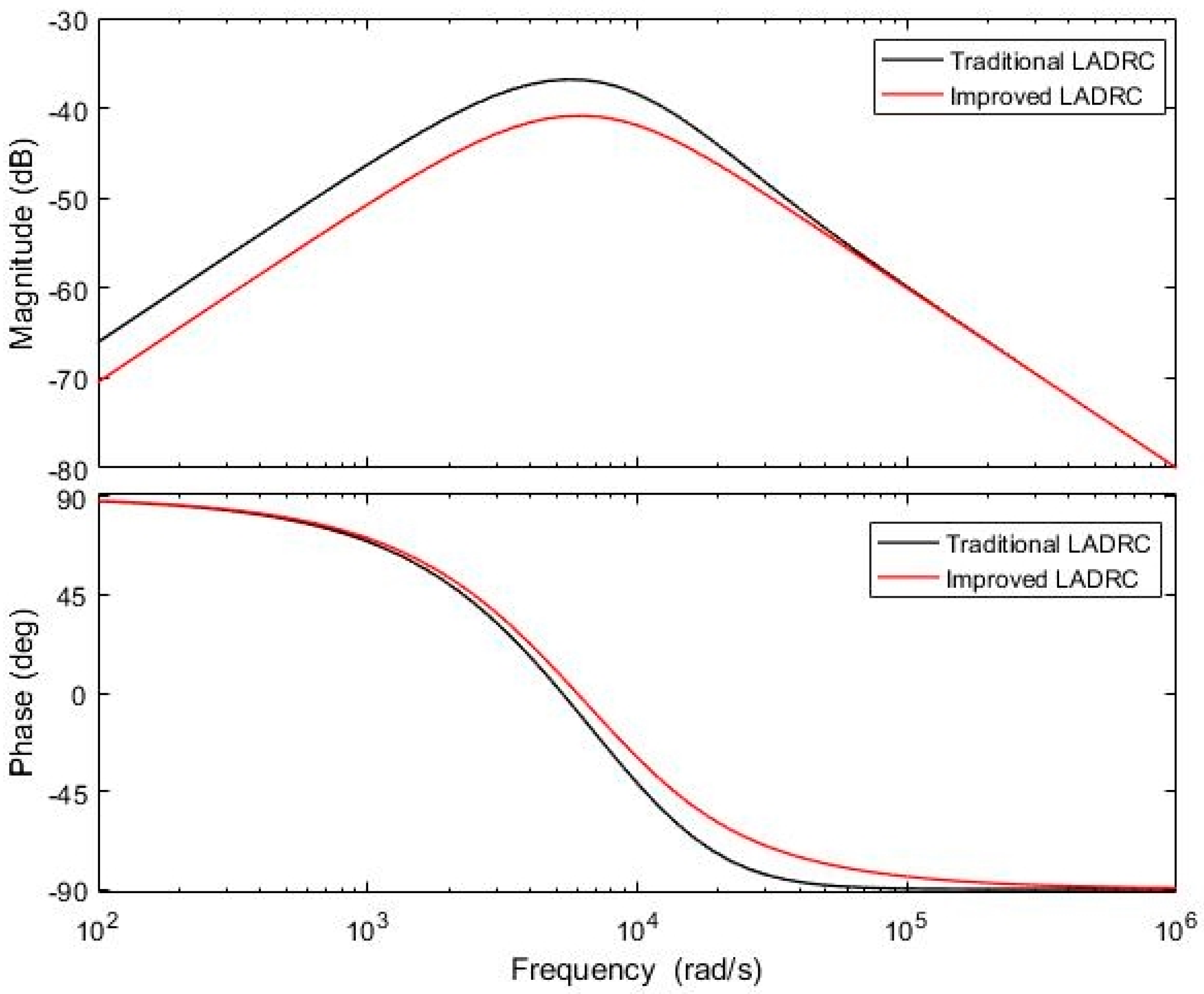
From Equation (46), it can be seen that the modified LADRC disturbance term, in combination with the D-STATCOM system, is only related to ${\omega }_0$ and ${\omega }_c$. Within the same system, the same ${\omega }_0$ and ${\omega }_c$ are identified. Figure 10 is a graph comparing the transfer function amplitude of disturbance terms between the improved LADRC and the traditional LADRC.

It can be seen from Figure 10 that the disturbance gain of the improved LADRC in medium- and low-frequency bands is significantly lower than that of the traditional LADRC, and the disturbance rejection ability of the improved LADRC is enhanced. It can be seen from the phase-frequency characteristics that the improved LADRC lags behind the traditional LADRC in phase, and the disturbance suppression ability is increased [23].

4.3.3. Stability Analysis of Improved LADRC in D-STATCOM System

According to Equation (46), the transfer function of the D-STATCOM system input items can be obtained:

$$i_d=\frac{{\omega }_c{\left(s+{\omega }_0\right)}^2}{a_1{s}^3+a_2{s}^2+a_{3}s+a_4}{i}_{d\_ref}$$

(49)

Among them:

$$\{\begin{array}{l}{a}_1=L{b}_0\\ a_2={\omega }_0+R{b}_0+L{b}_0\left({\omega }_0+{\omega }_c\right)\\ a_3={\omega }_0^2+\left(2{\omega }_c+R{b}_0\right){\omega }_0+R{b}_0{\omega }_c\\ a_4={\omega }_0^2{\omega }_c\end{array}$$

(50)

Observer bandwidth ${\omega }_0$ and controller bandwidth ${\omega }_c$ are positive, and the D-STATCOM system inductance $L$ is positive. It is easy to calculate that $a_1$ $a_2$ $a_3$ $a_4$ are positive. Then, according to the stability criterion of Lynard–Chiapart algebra, the necessary and sufficient conditions for system stability are:

$$\mathsf{\Delta }=\left|\begin{array}{ccc}{a}_2& a_4& 0\\ a_1& a_3& 0\\ 0& a_2& a_4\end{array}\right|=a_4\left(a_3{a}_2-a_1{a}_4\right)$$

(51)

According to the above equation, it can be seen that the third-order Hervitz discriminant of the system is greater than zero, namely $\mathsf{\Delta }>0$. So, the control system is stable [24].

5. Simulation and Experiment Analysis

In order to verify the effectiveness of the improved LADRC strategy described in this article, the article builds on the D-STATCOM simulation model shown in Figure 1 based on MATLAB and Simulink simulation software. When the D-STATCOM is used for reactive power compensation, the traditional LADRC control and the LADRC double closed-loop control mentioned in this article are utilized in three aspects: DC side voltage stability and harmonic distortion rate, grid side voltage drop reactive current tracking and power generated by the D-STATCOM during system load and load reduction. The compensation performance of the two different controllers is compared and analyzed. System parameters can be found in Appendix A.

5.1. Comparative Analysis of Steady-State Voltage on DC Side and Harmonic Distortion Rate

Given that the initial voltage of the system is 700 V, it can be seen from Figure 11 that the DC side voltage curve of the PWM converter controlled by the traditional LADRC has overshoot and fluctuation, while the DC side voltage curve controlled by the improved LADRC almost reaches the stable value without overshoot and oscillation.

It can be seen from Figure 12 that the harmonic distortion rate of the grid-connected current is greatly reduced when the improved LADRC control is adopted, and the harmonic content of the grid-connected current is reduced from 3.67% to 1.54%. The simulation results show that the improved LADRC plays a significant role in restraining the harmonic distortion rate of the grid current and improving the power quality of the grid, and also shows the effectiveness of the improved LADRC in controlling the D-STATCOM.

5.2. Comparative Analysis of Reactive Current Tracking Performance

To observe the tracking ability of the reactive current intuitively, as shown in Figure 13, the voltage balance drop of the system is set at 0.3 s, and the network voltage drops to 50% of the original value and returns to the original voltage steady state at 0.7 s. It can be seen from Figure 14 that when the improved LADRC control is applied, the actual reactive current $i_q$ can track $i_{q\_ref}$ almost without a difference and without lag. Compared with the traditional LADRC control, the improved LADRC has less fluctuation in tracking reactive current when measuring voltage drop, which proves that the improved LADRC has strong tracking ability.

5.3. Comparison and Analysis of the Output Power of D-STATCOM Under Load Change

The system is set to load 50% in 0.3 s and restore the original load in 0.7 s, which is taken as the system disturbance. It can be seen from Figure 15a that the adjustment time of traditional LADRC control is relatively long. The reactive power amplitude of the D-STATCOM fluctuates greatly, and the active power of the system greatly overshoots when the system is underloaded. As shown in Figure 15b, the improved LADRC has a fast adjustment time, and the reactive power issued by the D-STATCOM has almost no fluctuation when the load of the system is loaded or unloaded. The comparison analysis shows that the improved LADRC has stronger disturbance immunity.

5.4. Experimental Verification

The improved LADRC control method described in this paper is applied to a laboratory 20 kVAr experimental device. The available power factor values obtained from the control panel are shown in Figure 16b after curve fitting. It can be seen from the power factor fitting that the power factor of the system can quickly reach 1 and remain stable. This verifies the effectiveness of the improved LADRC.

6. Conclusions

In this paper, aiming at the nonlinear, multivariable, and strong coupling characteristics of the D-STATCOM, an improved LADRC control strategy is proposed to apply to the inner current loop and outer voltage loop of the D-STATCOM system. The key to the performance of the Linear Active Disturbance Rejection Controller is whether the extended state observer can accurately estimate the state variables of the system. The innovation of this paper is to propose a new deviation quantity to control the state variable of the LESO, to improve the control performance of the whole control system. The state variables of the traditional LESO only depend on a single deviation control, which causes the selected controller bandwidth and observer bandwidth to be too large and affects the dynamic performance of the controller. At the same time, it may amplify high-frequency noise, which makes the entire control system prone to high-frequency oscillations. Therefore, the next task of our research team is to resolve the contradiction between the controller and its sensitivity to noise, as well as physical experiments to support the theoretical analysis.

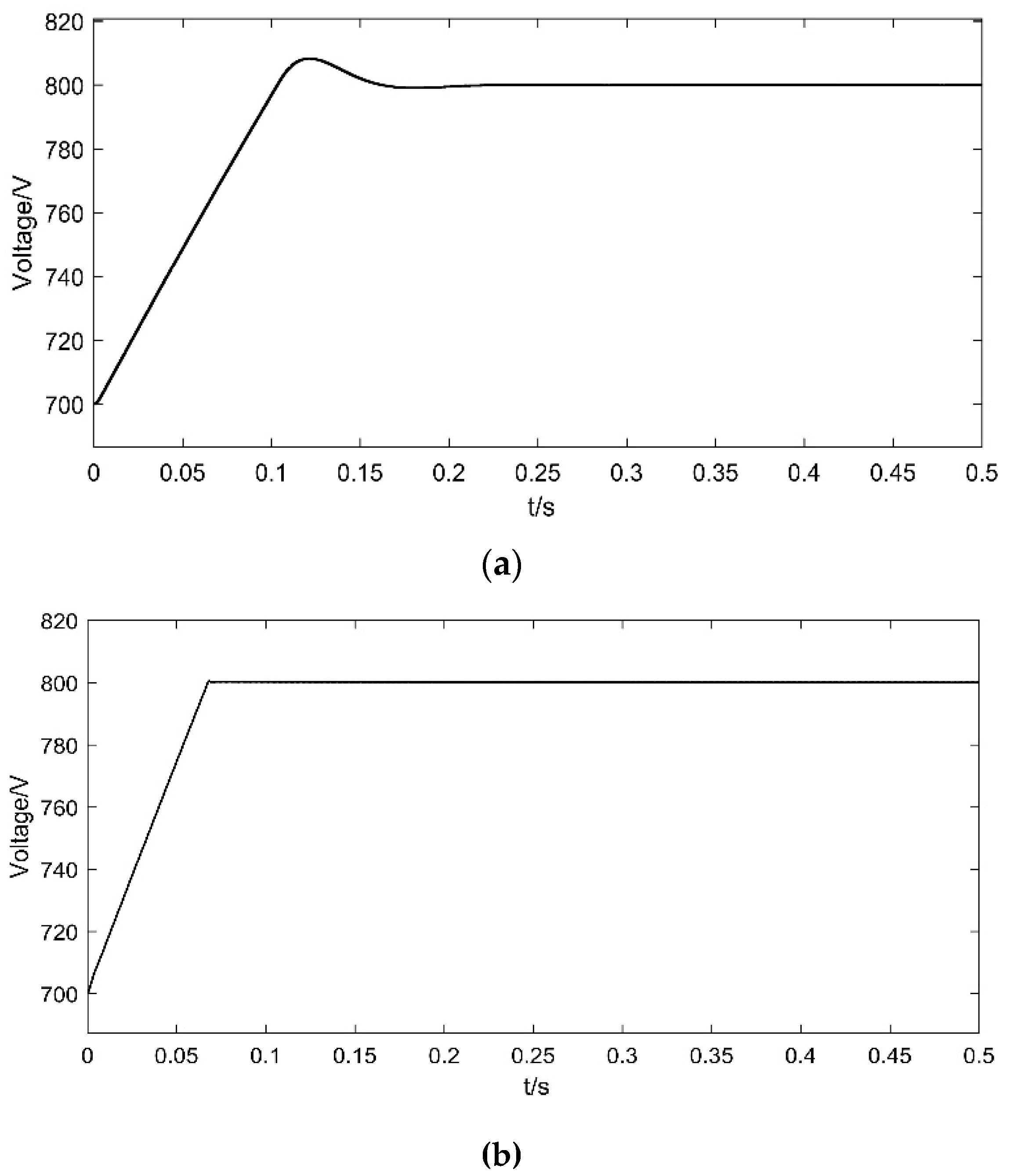
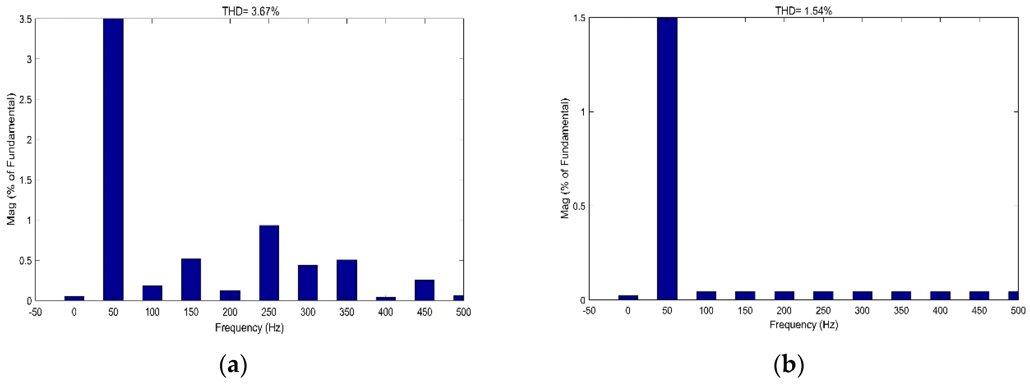
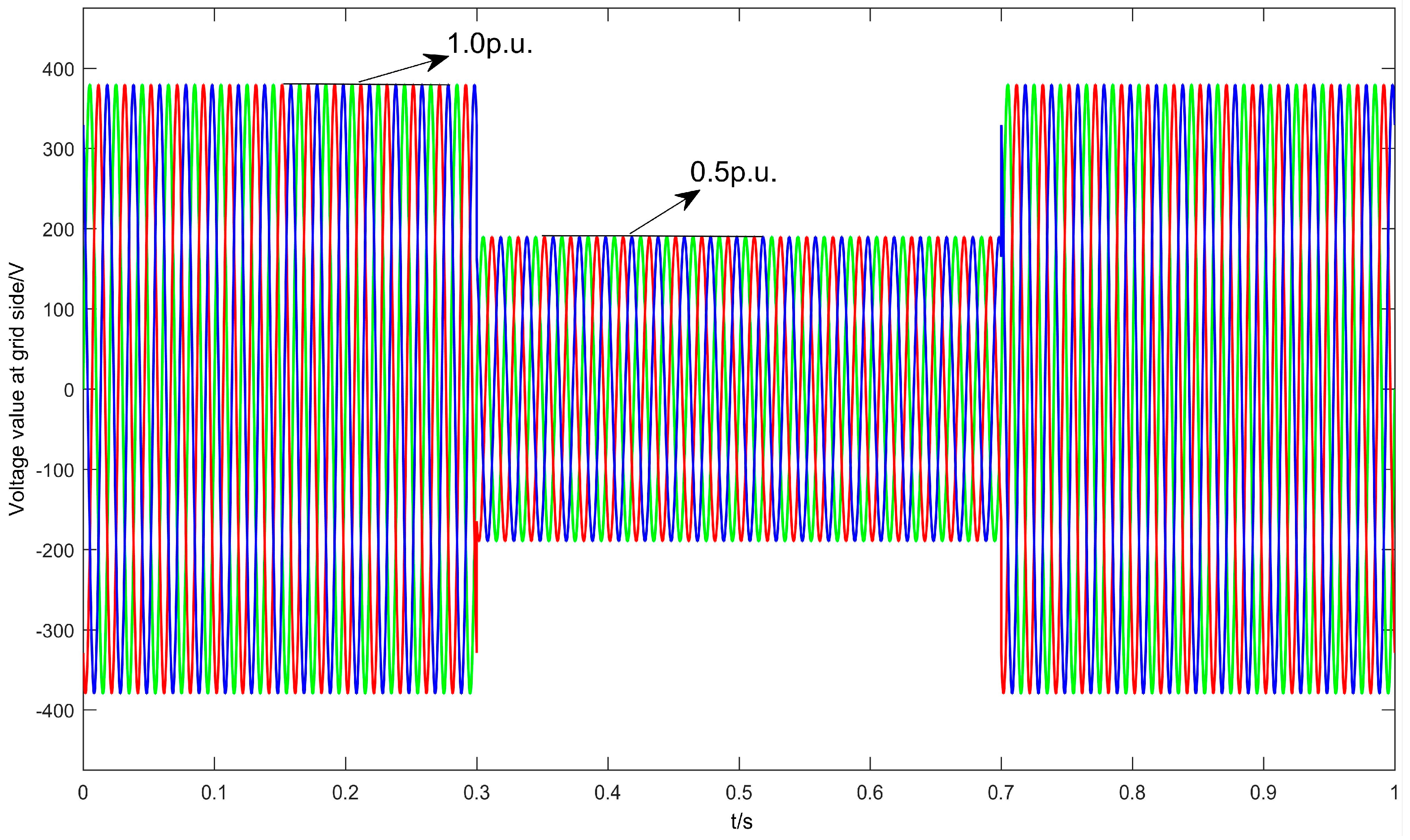
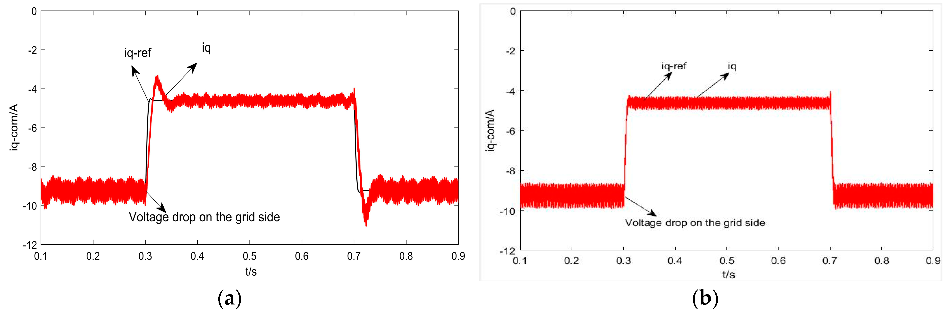
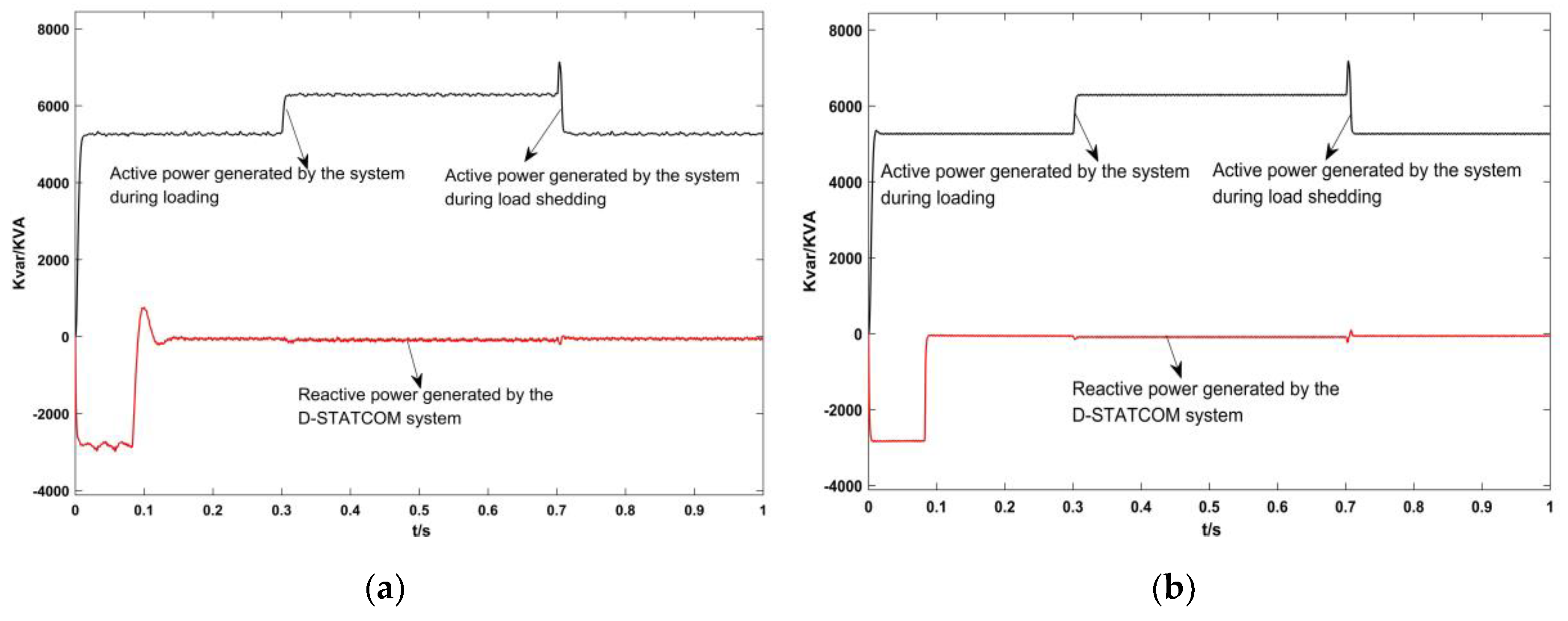
The specific work of this paper is as follows: Firstly, the mathematical model of the D-STATCOM is established, then a double closed-loop improved LADRC is proposed and designed by analyzing the traditional LADRC and the stability and anti-interference characteristics of the improved LADRC in the frequency domain in combination with the actual system. Finally, the simulation results show that the improved LADRC control has a faster and more stable dynamic performance than the traditional LADRC control when disturbed. Therefore, the improved LADRC can better solve the technical problems brought about by the D-STATCOM system’s total uncertain interference about D-STATCOM control and has good engineering practice value.