Abstract
This paper addresses the voltage control problem in medium-voltage distribution networks. The objective is to cost-efficiently maintain the voltage profile within a safe range, in presence of uncertainties in both the future working conditions, as well as the physical parameters of the system. Indeed, the voltage profile depends not only on the fluctuating renewable-based power generation and load demand, but also on the physical parameters of the system components. In reality, the characteristics of loads, lines and transformers are subject to complex and dynamic dependencies, which are difficult to model. In such a context, the quality of the control strategy depends on the accuracy of the power flow representation, which requires to capture the non-linear behavior of the power network. Relying on the detailed analytical models (which are still subject to uncertainties) introduces a high computational power that does not comply with the real-time constraint of the voltage control task. To address this issue, while avoiding arbitrary modeling approximations, we leverage a deep reinforcement learning model to ensure an autonomous grid operational control. Outcomes show that the proposed model-free approach offers a promising alternative to find a compromise between calculation time, conservativeness and economic performance.
1. Introduction
The massive integration of Distributed Generation (DG) units in electric distribution networks poses significant challenges for system operators [1,2,3,4,5]. Indeed, distribution networks were historically sized (with a radial structure) to meet maximum load demands while avoiding under-voltages at the end of the lines. However, in presence of local generation, the opposite over-voltage problem may appear. In case of severe voltage violation, inverters of DG units are temporarily cut off. This induces not only a loss of renewable-based energy, but also a deterioration of the delivered power quality (due to resulting voltage and current transients) that accelerates the equipment degradation [6]. In this context, the objective of modern Distribution System Operators (DSOs) is to adopt a reliable and cost-efficient strategy that is able to maintain a safe voltage profile in both normal and contingency conditions, with the goal of enhancing the ability of the system to accommodate new renewable-based resources. To that end, researchers have developed a wide range of techniques, with the aim of avoiding costly investment plans that simply upgrade/reinforce the network. Also, static (experience-based) strategies based on past observations have shown limitations, as they are often sub-optimal and unable to react in a very short time frame (to prevent cascading faults just after a disturbance) [7].
Theoretically, different methods can be applied for voltage management of Medium-Voltage (MV) distribution systems, but the most common methods are based on using on-load tap changer mechanism of the transformer, reactive power compensation and curtailment of DG active powers [8,9]. It is generally known that each of the above voltage control methods has its own advantages and drawbacks, and there is no single perfect voltage regulation method [10]. Recently, there has been a growing literature focusing purely on local strategies in which resources rely only on localized measurements of the voltages’ magnitude, and do not exchange information with other agents [11,12]. Such local algorithms are easy to implement in practice, but the lack of a global vision may prevent to cost-efficiently solve the voltage control problem. As an alternative, distributed strategies, which require communication capabilities between neighbouring agents, are also considered. Such approaches enable resources (that are physically close) to share information in order to cooperatively achieve the desired target levels, while considering other objectives such as losses minimization [13,14,15]. However, to further improve the optimality of the control solution, centralized voltage control algorithms, which are mainly based on an Optimal Power Flow (OPF) formulation, have also been proposed [16,17,18].
In general, although the latter centralized model-based techniques have shown promising performance, they are plagued with two main issues.
Firstly, they require to solve challenging optimization problems, which are non-linear and non-convex (from the AC power flow equations used to comply with the physical constraints of the electrical distribution system), and subject to uncertainties (from the stochastic load and generation changes, and the unexpected contingencies). The OPF-based methods thereby face scalability issues, which makes them of little relevance for real-time operation. This is partly addressed by using efficient nonlinear programming techniques [19], or through convex approximations of power flow constraints, which mainly resort on second order cone programs [20] or linear reformulations using the sensitivity analysis [21,22,23]. However, modeling errors inevitably arise and may lead to unsafe and sub-optimal solutions. Moreover, the recent trend of operating the modern distribution networks in closed loop mode makes traditional approximations even less accurate [24].
Secondly, the common feature of model-based techniques is that they assume that the physical parameters of the distribution networks are perfectly known, which is impractical due to the high complexity of these systems. In that regard, the real-time characteristics of the network components are not static, and are governed by complex dynamic dependencies [25]. For instance, deviations of parameters can arise from the atmospheric conditions and aging. Important effects are thereby often neglected, i.e., load power factors are not available precisely, there is a complex dependence structure between load and voltage levels, line impedances vary with the conductor temperatures, and the shunt admittances of lines as well as the internal resistance of transformers are also affecting network conditions [26].
The first issue (related to the high computational costs of model-based control algorithms) has led to the implementation of reinforcement learning (RL). These data-driven methods have the advantage to directly learn their operating strategy from historical data in a model-free fashion (without any assumptions on the functional form of the model). Consequently, they can show good robustness under very complex environments with measurement noise [27,28]. A novel deep reinforcement learning (DRL)-based voltage control scheme (named Grid Mind) is developed in [29]. In particular, two different techniques have been compared, i.e., deep Q-network (DQN) and deep deterministic policy gradient (DDPG), and both have shown promising outcomes. In [30], voltage regulation is improved using a RL-based policy that determines the optimal tap setting of transformers. Then, a new voltage control solution combining actions on two different time scales is implemented in [31], where DQN is applied for the (slow) operation of capacitor banks. Finally, multi-agent frameworks have been developed in [32,33] to enable decentralized executions of the control procedure that do not require a central controller.
However, all these methods are disregarding the endogenous uncertainties on network parameters, which may mislead the DSO into believing that the control strategy satisfies technical constraints, while it may actually result into unsafe conditions. In this context, the main contribution of this paper is to propose a self-learning voltage control tool based on deep reinforcement learning (DRL), which accounts for the limited knowledge on both the network parameters and the future (very-short-term) working conditions. The proposed tool can support DSOs in making autonomous and quick control actions to maintain nodal voltages within their safe range, in a cost-optimal manner (through the optimal use of ancillary services in a market environment). In this work, it is assumed that for voltage control purpose, we can act on the active and reactive powers of DG units as well as on the transformer tap position. The resulting problem is formulated as a single-agent centralized control model.
The main advantage of the proposed method lies in its ability to learn from scratch (in an off-line fashion) and gradually master the system operation. Hence, the computational burden is transferred in pre-processing (when the model is calibrated/learned through many simulations), such that the real-time control process (in actual field operation when the agent is trained) is insignificant (≪1 s). Also, the model-free tool allows to immunize the voltage control procedure against uncertainties in both exogenous (load conditions) and endogenous (network parameters) variables, while accounting for approximations in the power flow models describing the system operation. Results from a case study on a 77-bus, 11 kV radial distribution system reveal that the proposed tool allows determining an optimal policy that lead to safe grid operation at low costs.
The remainder of this paper is organized as follows. Section 2 introduces the theoretical background in reinforcement learning, with a particular interest on the deep deterministic policy gradient (DDPG) algorithm, which allows to handle high-dimensional (and continuous) action spaces. Section 3 describes the simulation environment, including the different sources of uncertainty. The developed method is tested (using new representative network conditions) in Section 4 on a realistic 77-bus system, where we validate its robustness through the numerical simulations. Finally, conclusions and perspectives for future research are given in Section 5.
2. Reinforcement Learning Background
In this section, we introduce the basics of reinforcement learning (RL), while making the practical connections with the voltage control problem.
2.1. Markov Decision Process
Firstly, the problem has to be formulated as a Markov Decision Process (MDP). The general principle consists of an agent interacting with an environment over a number of discrete time steps until the agent reaches a terminal state. In particular, at each step t, the agent observes a state from the state space , and selects an action according to its policy . As a result, the agent ends up in the next state while receiving an immediate scalar reward based on the distribution in accordance with the natural laws of the environment. The next state depends only on the action on state (and not on the prior history), which is a characteristic referred to as the Markov property.
In this work, the agent is the central controller which regulates the voltage level within its control area, and the environment is the electrical distribution network (including the realization of the different sources of uncertainty affecting its operation). The state-transition model and the reward function are inherently stochastic, and the problem can thus be formulated using reinforcement learning.
2.1.1. State Space
The state space of the RL agent (i.e., central controller) is defined by the information that can be measured in real-time by SCADA (Supervisory Control and Data Acquisition) or PMU (Phasor Measurement Unit). In that regard, the state space at time t contains the voltage levels for each node of the distribution system. Then, this information is complemented by the (predicted) maximum power level of each distributed generators at the next time interval . This information (reflecting, e.g., the maximum energy contained in the wind) allows the agent to know the upper limit of these control variables when taking its actions. Practically, this is achieved using a (deterministic) single-step ahead forecaster, which is based on an advanced architecture of recurrent neural networks, as presented in [34]. The latter is tailored to predict the power level in the upcoming future by leveraging the past dynamics of the generator output. Finally, the current tap position of the transformer (which defines the turn ratio between primary and secondary voltage levels) is also included in the state space .
2.1.2. Action Space
The action space to fix voltage issues in the studied network consists in changing the active and reactive powers of DG units, i.e., and , as well as adjusting the transformer tap ratio .
The actual changes in active and reactive power levels initiated at time t (which will define the power output at time ) are limited by the available power at time :
where denotes the power level of (dispatchable) generator g at time t, while and determine the safe range of variation of reactive power of unit g around the operation point. Likewise, the variation around the operation point of the transformer tap change is given by:
where and are the physical limits of the on-load tap changer.
It should be noted that other types of control actions, such as changing the terminal voltage set-points of (medium-sized) conventional generators or switching shunt devices, could also be considered if such resources are available in the system.
2.1.3. Reward
As the goal of the algorithm is to eliminate voltage issues at a minimal cost, the reward includes both the costs inherent to control actions (changing set-points of control variables, which may reflect the costs of relying on ancillary services [35]), and the costs of violating network constraints (which may damage the equipment). In this way, the immediate reward at time step t is defined as follows:
where and are respectively the lower and upper bounds delimiting the safe voltage levels. Then, coefficients and represent the costs of modifying the active and reactive powers of DG units, while stands for the (high) cost of changing the transformer tap position. Typically, we have . Indeed, modifying the reactive power of generators can be done at almost no cost (using the power electronics converters), while the curtailment of active power infers a loss of generated energy that ultimately results into a financial loss [36]. Then, high costs are associated with a tap change of the transformer due to the aging effects on the tap changer contacts. The terms and respectively reflect the positive reward for the nodes having voltages within the safe range, and the negative reward (i.e., penalty) for nodes outside the permitted zone. In general, all these costs need to be properly weighted (see Section 4). Indeed, if the costs of actions , and are too high with respect to and , the agent may choose to suffer the negative rewards related to voltage violations (rather than correcting the voltage problem). Conversely, if the costs of actions are too low, unnecessary actions may be taken (to ensure the positive rewards related to safe voltage levels).
2.2. Reinforcement Learning Algorithm
Like most machine learning techniques, it is important to differentiate training and test stages.
During the training, the goal of the agent is to learn the best policy , i.e., to select actions that maximize the cumulative future reward with a discount factor . This can be achieved by approximating the optimal action-value function , which is the expected discounted return of taking action a in state s, then continuing by choosing actions optimally. Indeed, once -values are obtained, the optimal policy can be easily constructed by taking the action given by . Using Bellman’s principle of optimality, can be expressed as
where the next state is sampled from the environment’s transition rules . In general, an agent starts from an initial (poor) policy that is progressively improved through many experiences (during which the agent learns how to maximize its rewards).
When the training is completed, i.e., during the test (in practical field operations), the trained agent selects the greedy action according to its learned policy.
This general principle is the source of many different RL algorithms, each with different characteristics that suits different needs. In this context, the choice of the most suited technique for the voltage control task is mainly driven by the fact that both state and action spaces are continuous. Hence, well-known algorithms, such as (deep) Q-learning, will not be considered as they only deal with a discrete action space. In this work, we will thereby focus on the deep deterministic policy gradient (DDPG) technique.
2.3. Deep Deterministic Policy Gradient (Ddpg) Algorithm
The deep deterministic policy gradient (DDPG) relies on a complicated architecture, referred to as actor-critic [37], which is depicted in Figure 1. The goal of the actor is to learn a deterministic policy which selects the action a based on the state s. The quality of the action is estimated by the critic, by computing the corresponding . To achieve good generalization capabilities of both actor and critic functions, they are estimated using deep neural networks, which are universal non-linear approximators that are very robust when the state and action spaces become large.
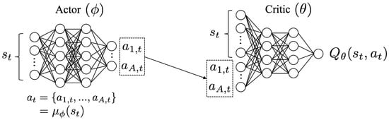
Figure 1.
Working principle of the DDPG agent, which relies on an actor-critic architecture.
Overall, starting from an initial state s, the actor neural network (characterized by weight parameters ) determines the action . This action is then applied to the environment, which yields the reward and the next state . The experience tuple is then stored in the replay memory. Once the replay memory includes enough experiences, a random mini-batch of D experiences is sampled. For each sample in the mini-batch, the state and the action are fed into the critic neural network (characterized by weight parameters ) that yields the Q-value. Both networks are then jointly updated, and the procedure is iterated until convergence.
Practically, the critic network is trained by adjusting its parameters (at regular intervals during the learning phase) so as to minimize the mean-squared Bellman error (MSBE) (9). In contrast to supervised learning, the actual (i.e., optimal) target value is unknown, and is thus substituted with an approximate target value (using the estimation ):
where is given by the critic network, i.e., .
Contrary to supervised learning where the output of the neural network and the target value (i.e., ground truth) are completely independent, we see that the target value y in (8) depends on the parameters and that we are optimizing in the training. This link between the critic’s output and its target may infer divergence in the learning procedure. A solution to this problem is to use separate target networks (for both the critic and the actor), which are responsible for calculating the target values. Practically, these target networks are time-delayed copies of the original networks with parameters and that slowly track the (reference) learned networks. As explained in [37], these target networks are not trained, and enable to break the dependency between the values computed by the networks and their targeted value, thereby improving stability in learning.
As a result, the critic network is trained (i.e., updated) by minimizing the following MSBE loss function with stochastic gradient descent:
Starting from random values , the parameters are thus progressively updated towards the optimal action-value function by minimizing the difference between (i) the output of the critic and (ii) the target (computed with target networks), which provides an estimate of the Q-function using both the outcome of the simulation model and the action from the target actor network. The update is performed on a mini-batch D of different experiences , drawn uniformly at random from the pool of historical samples. This (replay buffer) procedure breaks the similarity between consecutive training samples, thus avoiding that the model is updated towards a local minimum.
In parallel, the actor network is trained (on the same mini-batch D) with the goal of adapting its parameters , so as to provide actions that maximize . This amounts to maximize the following function , which is achieved with a gradient ascent algorithm:
To ensure that the DDPG algorithm properly explores its environment during the training phase, noise is added to the action space, i.e., . In particular, we use an exponential decaying noise so as to favor exploration at the start of the training, which is then progressively decreased to stimulate exploitation as the agent converges towards the optimal policy. Naturally, when the model is trained (and used during test time), no noise is added to the optimal action .
3. Simulation Environment
To train the DRL agent, it is necessary to build a simulation environment that mimics the actual system. This environment is composed of three modules: (i) to generate realistic deviations of the expected nodal load and distributed generation powers for the next time step (to reflect prediction errors), (ii) to provide realistic values of the uncertain network parameters, and (iii) to simulate the physical flows in the distribution network.
As depicted in Figure 2, the RL agent is trained off-line through interactions with the simulation environment, which allows calibrating the RL model using experience and rewards. As previously explained, the starting point is an observation of the state of the environment (e.g., nodal voltage levels of the distribution system). Based on this information, the (target) actor network is used to take an action (where the additional noise is used during training to boost exploration). It should be noted that, if no voltage problem is observed, the optimal action is to do nothing. Then, the simulator (thoroughly described in the rest of this Section) is used to determine the impact of the action on the environment, which consists in computing the reward , but also the next state . Then, the (target) critic is used to evaluate the quality of the decisions, and both actor and critic networks are updated using respectively (10) and (9) to improve the policy of the DRL-based agent.
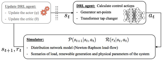
Figure 2.
Training of the DRL agent for autonomous voltage control in distribution systems.
When the learning is performed, the agent can be deployed for practical power system operation (for which only the actor network is useful). Interestingly, the agent can still continue its learning (and thus adapt to potential misrepresentations of the simulation environment) by adjusting its parameters through on-line feedback. This may also serve for calibrating the model to the time-varying conditions of the system.
3.1. Exogenous Uncertainties on the Network Operating Point
The first category of uncertainties belongs to the network working point (regarding both the nodal consumptions and generations). Indeed, the output power of renewable-based generators is intermittent upon the nature of their primal sources (mainly wind and solar), such that the generated power can quickly vary within a short interval. Moreover, the nodal consumption and generation levels are not always measurable. Consequently, in practice, the future operating state of the distribution system is not known with certainty, and this stochasticity is here represented with scenarios of representative prediction errors. Practically, for the renewable generation, a database is constructed based on the historical prediction errors of the employed forecaster (described in Section 2.1.1), and a sample is randomly drawn from this database to generate the desired scenario. For the nodal loads, the same sampling strategy is used to simulate the (uncertain) changes in the consumption level.
3.2. Endogenous Uncertainties on the Network Component Models and Parameters
The second category of uncertainties is related to partial knowledge of network component models and parameters. In general, network analyses and simulations are carried out relying on the simplified models of network components, which do not correctly represent the physical relations and dependencies within the real network. This includes uncertainties associated with the line, load and transformer models [26].
In particular, we model the thermal dependency phenomenon whereby the line resistance fluctuates with respect to the conductor temperature variation. Then, the uncertainty associated with the load power factor is considered to better reflect the different natures, types and amplitudes of the various load demands. Moreover, as shown in [38], the internal resistance of the transformer can have a significant effect on the node voltages, and is thereby also incorporated in the network model. Finally, in contrast to typical network models, the shunt admittances of power lines are taken into account using the PI line model. Overall, all these (uncertain) parameters are modelled as random variables changing within representative predefined bounds.
3.3. Distribution Network Model
The electrical network operation is modeled through load-flow calculations, which are solved using the Newton-Raphson approach.
4. Case Study
To solve the voltage control problem, the DDPG algorithm is implemented in Python using PyTorch and Gym libraries. The solution is tested on the 11 kV radial distribution system with N = 77 buses shown in Figure 3 [39]. The bus 1 is the high-voltage (HV) connection point, which is considered as the slack node. The substation (between nodes 1 and 2) supplies 8 different feeders, for a total of 75 loads. The maximum (peak) active and reactive consumption powers equal to 24.27 MW and 4.85 Mvar, respectively. The system is also hosting 22 (identical) distributed generators, with an installed power equal to 4 MW.
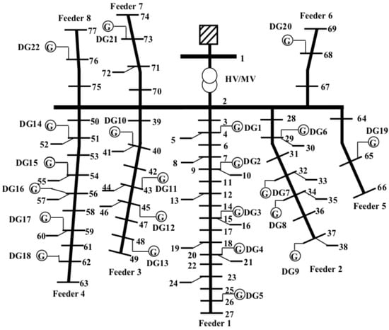
Figure 3.
Schematic diagram of the 77-bus distribution system. The section between bus 1 and 2 is the substation, which is supplying 8 different feeders.
The objective of the DRL-based agent is to maintain the voltage magnitudes of the 77 buses within the desired range. In order to illustrate the effectiveness of the proposed control scheme, these allowed voltage limits are defined by a very conservative range of [0.99, 1.01] p.u., and the initial reactive powers of DGs are set to zero. The reward function (6) is characterized by a compromise between the costs of voltage violations and those of corrective actions. We give more weight in maintaining safe voltage levels by defining and , while , and are respectively set to 1, 0.1 and 0.04.
A total of 12,000 initial operating states (that need to be processed by the DRL-based agent) are generated with the simulation model, among which 10,000 are used to train the agent, while the remaining 2000 scenarios are kept (as a test set) to evaluate the performance of the resulting model. It should be noted that, in this work, the agent has a single step to process each of the generated scenarios (it cannot rely on several interactions with the environment to solve a voltage problem). The value of the discount factor is thereby fixed to 1.
To have an overview of the global network conditions in the case where no control action is performed, we show in Figure 4 the distribution of nodal voltage levels (for the 12,000 simulated states) using a boxplot representation. We observe that violations of voltage limits [0.99, 1.01] p.u. occur more than 50% of the time. In particular, the distribution is asymmetrical, skewed towards more over-voltage issues (due to the high penetration of distributed generation) which occurs in 40.1% of the simulated samples.
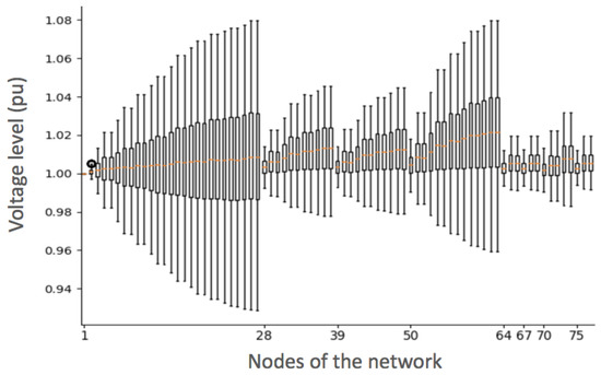
Figure 4.
Boxplot representing the (nodal) distributions of the voltage levels for the 77 buses among the 12,000 simulated states.
4.1. Impact of Ddpg Parameters
In the proposed case study, the state space is of size 100, i.e., 77 dimensions for the nodal voltages , 22 dimensions for the (predicted) maximum power of the 22 generators , and 1 dimension for the position of the tap changer . Also, the action space is of size 45, i.e., 2 × 22 = 44 dimensions corresponding to the changes in active and reactive power for the 22 generators, and 1 dimension for changing the position of the tap changer. Hence, as sketched in Figure 5, the actor network has an input layer of size 100 (i.e., composed of 100 neurons), and an output layer of size 45. Then, the critic network is characterized by 145-dimensional input layer, for a single output.
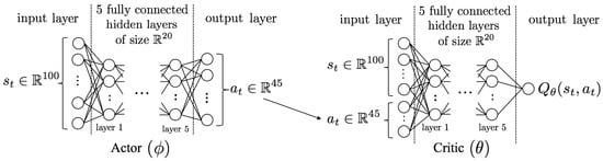
Figure 5.
Representation of the neural network architectures for both actor and critic.
Based on this (fixed) information, we then performed an optimization of the hyper-parameters of the DRL-based agent, which consists in optimizing its complexity by adding extra hidden layers in the architecture of both actor and critic neural networks. In particular, the best performance was achieved by connecting the input and output layers (for both the actor and the critic networks) with 5 fully connected layers, with 20 units in all layers. The activation functions of the hidden layers are ReLU (rectified linear units). Then, the hyperbolic tangent function is used for the output layer of the actor, while a linear function is employed for the critic. The batch size of the learning is set to 16 samples, and the target networks are updated (during the training) with a delay of 10 iterations. Both actor and critic networks are initialized with random weights in the range [, 0.1].
The exploration-exploitation parameter (i.e., extra noise added to the actions during the training) is , where is a zero-mean Gaussian noise with a standard deviation of 0.2, which is exponentially decaying along the training iterations k. The decay period is equal to 5000 episodes. In general, this action noise has a significant impact on the learning abilities of the DRL-based agent. This observation is illustrated in Figure 6, where we depict two different learning curves where all parameters of the agents are similar, except for the action noise. In particular, the optimal calibration of is compared to a perturbation of (with the same decaying intensity over the training samples).
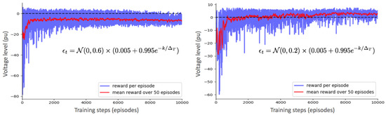
Figure 6.
Evolution of the total immediate rewards across training episodes for two different configurations of the action noise .
In general, when the perturbations are too small, the training may fail to properly explore the search space (which increases the probability to end up in a local minimum), while oversized perturbations may negatively affect the learning (and even leading the algorithm to repeatedly perform the same action).
For the best model (right part of Figure 6), we see that the DDPG control scheme quickly learns (after around 7500 interactions with the environment) a stable and efficient policy. In particular, at the beginning (during the 2000 first training steps), the agent randomly selects actions, which lead to many situations where it deteriorates the electrical network conditions. However, in the course of the learning procedure, the agent is progressively evolving, and starts solving the voltage issues with less costly decisions. The agent eventually converges to total rewards . In contrast, the other model (left part of Figure 6) achieves convergence at a much lower performance (total rewards of ), which roughly corresponds to the same reward as when no action is performed. In general, the main advantage of the proposed framework lies in its generic design that makes it broadly applicable (e.g., to any distribution system), and in its ability to adapt to the varying operating conditions. Evidently, when the methodology is applied to another environment, the DDPG agent needs to be re-trained from scratch, and its hyper-parameters (e.g., training noise, as well as number of hidden layers and number of neurons for both actor and critic networks) also need to be adapted.
4.2. Impact of Endogenous Uncertainties
The impact of endogenous uncertainties (regarding the physical parameters of the distribution system) is evaluated through the analysis of three cases.
- The network parameters are considered as perfectly known in both training and test stages;
- The uncertainty on the network parameters are neglected during the training phase (to mimic current optimization models), but are considered when evaluating the performance of the trained DRL-based agent (to reflect reality);
- The uncertainty on the values of network parameters is accounted for in both training and test phases.
The simulation results regarding the three cases are summarized in Figure 7. Practically, we represent the evolution of the negative reward (which is a measure of the voltage violations) in both training and test phases. This negative reward is equal to 0 in the perfect situation where all nodal voltages pertain to = [0.99, 1.01] p.u., and decreases in negative values with the severity of voltage violations, i.e.,:
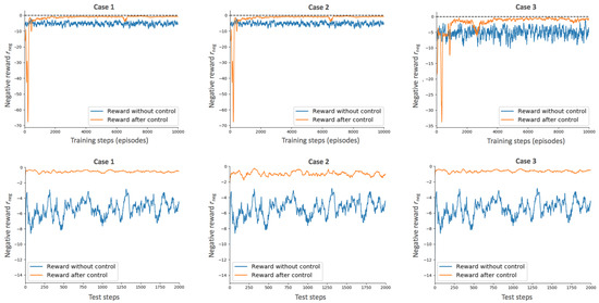
Figure 7.
Evolution of the reward in the three studied cases in both training and test stages.
We observe that when uncertainties associated with the model parameters are neglected during the training (cases I and II), the RL agent quickly find actions that remove voltage violations, i.e., the upper bound of the negative reward is almost reached in around 2000 episodes. This performance is achieved in more than 4000 episodes when dealing with endogenous uncertainties due to the increased difficulty of the task. This effect is also translated into a higher variability of the reward. Interestingly, by comparing the evolution of with the total reward r in Figure 6 during the training, we see that even though the agent is able to mitigate the voltage issues after 4000 training episodes, the cost-efficiency of the actions can still be improved (which is realized during the next 4000 episodes).
To quantify the impact of neglecting the endogenous model uncertainties, the mean value of the negative reward in (11) over the last 2000 episodes of the training phase, and over the 2000 new episodes of the test set are provided in Table 1 for the three studied cases.

Table 1.
Average value of the negative reward across training and test sets.
As expected, the agent that is agnostic to endogenous uncertainties on the physical parameters of the system during the training (cases 1 and 2) achieves a lower out-of-sample performance when these effects are modeled in the test set. Specifically, the reward drops from −0.53 (in case 1 when endogenous uncertainties are also disregarded at the test stage) down to −0.93 in the realistic case 2. In this latter situation, the agent expects a reward of around −0.6 (at the end of its learning), while it actually results in a disappointing ex-post outcome of −0.93. This problem can be efficiently alleviated by incorporating these endogenous uncertainties within the learning procedure. In that framework (case 3), the training and test rewards are close to each other, i.e., , which illustrates the good performance of the proposed method.
4.3. Extreme Cases
In this part, the outcome of the DRL-based agent is illustrated for two extreme situations, respectively corresponding to the worst-case over- and under-voltage states. These states result from the combination of extreme consumption and generation conditions, associated with unfavourable parameters of the distribution system (such as high line impedances arising from a temperature increase).
In Figure 8, we select the scenario (from the 2000 test samples) which leads to the worst-case voltage rise. In this case, the load demands are low (globally equal to around 10% of their nominal values) while active powers of DGs are at 90% of their rated values. The initial system voltages significantly exceed the upper limit of 1.01 p.u. (for almost all nodes), and reach a maximum value of 1.08 p.u. at node 27 (end of feeder 1). Also, the absolute value of the reward associated with the control actions taken by the proposed DDPG algorithm is represented in the right part of the Figure 8.
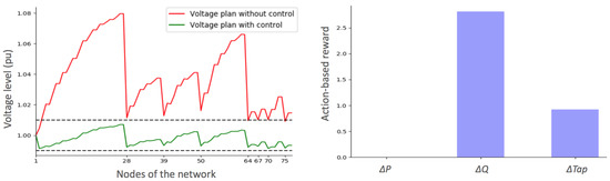
Figure 8.
Initial nodal voltages as well as the corrected ones obtained by the DRL-based agent in an extreme over-voltage situation. The corresponding (absolute value) of the reward related to each family of actions is also displayed.
Interestingly, the DRL-based agent has completely solved the voltage problem. We see that it did not rely on the curtailment of the active power of distributed generators. Indeed, this solution is more expensive than consuming reactive power (which is thereby the privileged action). However, the transformer tap ratio had also to be modified (i.e., voltage drop between nodes 1 and 2) to prevent over-voltages at the end of the feeders.
In Figure 9, the voltage drop condition is analyzed, which corresponds to a situation where load demands are maximum, while active powers of DGs are equal to zero. This results into under-voltage issues in many nodes of the distribution system.
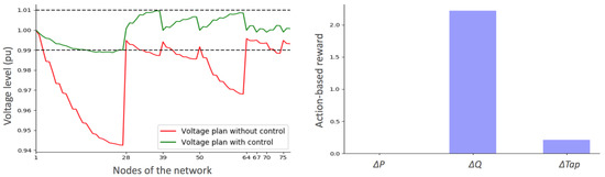
Figure 9.
Initial nodal voltages as well as the corrected ones obtained by the DRL-based agent in an extreme under-voltage situation. The corresponding (absolute value) of the reward related to each family of actions is also displayed.
Similarly to the over-voltage case, the privileged action is to modify the reactive power level of DG units (here by exchanging capacitive reactive power to compensate the voltage drops). The corrected situation brings the voltage plan within the desired limits, at the exception of some nodes at the end of feeder 1 that are slightly violating the lower bound (of 0.99 p.u.).
In general, after the training, the agent is able to successfully make the right decisions. In particular, during the testing under new randomly generated conditions, the proposed DRL-based algorithm achieves robust solutions (against the various sources of uncertainty) that mitigate severe voltage violations using cost-effective actions.
5. Conclusions and Perspectives
This paper was devoted to the voltage control problem in distribution systems, which is facing new challenges from growing dynamics and uncertainties. In particular, current strategies are hampered by the limited knowledge of the network parameters, which may prevent achieving the optimal cost-efficiency. This problem is formulated as a centralized control of resources using deep reinforcement learning, through an actor-critic architecture that enables to properly represent the continuous environment. This framework bypasses the need to represent analytically the electrical system, such that the impact of model accuracy is decoupled from the control performance.
The main advantage of the proposed model is to put the computational complexity on the pre-processing (in a fully data-driven framework), such that the model provides very fast decisions in test time. Interestingly, the developed regulation scheme is not only easy to implement, but also cost-efficient as we observe that the agent is able to automatically adapt its behavior to varying conditions.
The promising outcomes of the work pave the way towards more advanced strategies, such as the extension to a decentralized approach using a multi-agent formulation (that would prevent the single point of failure of the centralized framework). Similarly, extending the framework to partially observable networks (where the state of the system is not fully known [40]) also offers a valuable area of research for system operators.
Author Contributions
Conceptualization, J.-F.T. and F.V.; methodology, J.-F.T.; validation, J.-F.T., and B.B.Z.; writing–original draft preparation, J.-F.T. and B.B.Z.; writing–review and editing, M.H., Z.D.G. and F.V.; supervision, F.V.; project administration, F.V. All authors have read and agreed to the published version of the manuscript.
Funding
This research received no external funding.
Acknowledgments
J.-F. Toubeau is supported by FNRS (Belgian National Fund of Scientific Research).
Conflicts of Interest
The authors declare no conflict of interest.
References
- Toubeau, J.-F.; Vallée, F.; Grève, Z.D.; Lobry, J. A new approach based on the experimental design method for the improvement of the operational efficiency in Medium Voltage distribution networks. Int. J. Electr. Power Energy Syst. 2015, 66, 116–124. [Google Scholar] [CrossRef]
- Wei, B.; Deconinck, G. Distributed Optimization in Low Voltage Distribution Networks via Broadcast Signals. Energies 2020, 13, 43. [Google Scholar] [CrossRef]
- Klonari, V.; Toubeau, J.-F.; Lobry, J.; Vallée, F. Photovoltaic integration in smart city power distribution: A probabilistic photovoltaic hosting capacity assessment based on smart metering data. In Proceedings of the 2016 5th International Conference on Smart Cities and Green ICT Systems (SMARTGREENS), Rome, Italy, 23–25 April 2016; pp. 1–13. [Google Scholar]
- Liu, H.J.; Shi, W.; Zhu, H. Distributed voltage control in distribution networks: Online and robust implementations. IEEE Trans. Smart Grid 2018, 9, 6106–6117. [Google Scholar] [CrossRef]
- Ou-Yang, J.-X.; Long, X.-X.; Du, X.; Diao, Y.-B.; Li, M.-Y. Voltage Control Method for Active Distribution Networks Based on Regional Power Coordination. Energies 2019, 12, 4364. [Google Scholar] [CrossRef]
- Klonari, V.; Toubeau, J.-F.; Grève, Z.D.; Durieux, O.; Lobry, J.; Vallée, F. Probabilistic simulation framework for balanced and unbalanced low voltage networks. Int. J. Electr. Power Energy Syst. 2016, 82, 439–451. [Google Scholar] [CrossRef]
- Sun, H.; Guo, Q.; Qi, J.; Ajjarapu, V.; Bravo, R.; Chow, J.; Li, Z.; Moghe, R.; Nasr-Azadani, E.; Tamrakar, U.; et al. Review of challenges and research opportunities for voltage control in smart grids. IEEE Trans. Power Syst. 2019, 34, 2790–2801. [Google Scholar] [CrossRef]
- Xiao, C.; Sun, L.; Ding, M. Multiple Spatiotemporal Characteristics-Based Zonal Voltage Control for High Penetrated PVs in Active Distribution Networks. Energies 2020, 13, 249. [Google Scholar] [CrossRef]
- Xiao, C.; Zhao, B.; Ding, M.; Li, Z.; Ge, X. Zonal Voltage Control Combined Day-Ahead Scheduling and Real-Time Control for Distribution Networks with High Proportion of PVs. Energies 2017, 10, 1464. [Google Scholar] [CrossRef]
- Zad, B.B.; Lobry, J.; Vallée, F. A Centralized approach for voltage control of MV distribution systems using DGs power control and a direct sensitivity analysis method. In Proceedings of the IEEE International Energy Conference (ENERGYCON), Leuven, Belgium, 2–4 April 2016. [Google Scholar]
- Calderaro, V.; Conio, G.; Galdi, V.; Massa, G.; Piccolo, A. Optimal Decentralized Voltage Control for Distribution Systems With Inverter-Based Distributed Generators. IEEE Trans. Power Syst. 2014, 29, 230–241. [Google Scholar] [CrossRef]
- Nowak, S.; Wang, L.; Metcalfe, M.S. Two-level centralized and local voltage control in distribution systems mitigating effects of highly intermittent renewable generation. Int. J. Electr. Power Energy Syst. 2020, 119, 1–15. [Google Scholar] [CrossRef]
- Brenna, M.; Berardinis, E.D.; DelliCarpini, L.; Foiadelli, F.; Paulon, P.; Petroni, P.; Sapienza, G.; Scrosati, G.; Zaninelli, D. Automatic distributed voltage control algorithm in smart grids applications. IEEE Trans. Smart Grid 2013, 4, 877–885. [Google Scholar] [CrossRef]
- Almasalma, H.; Claeys, S.; Mikhaylov, K.; Haapola, J.; Pouttu, A.; Deconinck, G. Experimental Validation of Peer-to-Peer Distributed Voltage Control System. Energies 2018, 11, 1304. [Google Scholar] [CrossRef]
- Vovos, P.N.; Kiprakis, A.E.; Wallace, A.R.; Harrison, G.P. Centralized and Distributed Voltage Control: Impact on Distributed Generation Penetration. IEEE Trans. Power Syst. 2007, 22, 476–483. [Google Scholar] [CrossRef]
- Capitanescu, F.; Bilibin, I.; Ramos, E.R. A comprehensive centralized approach for voltage constraints management in active distribution grid. IEEE Trans. Power Syst. 2013, 29, 933–942. [Google Scholar] [CrossRef]
- Robertson, J.G.; Harrison, G.P.; Wallace, A.R. OPF Techniques for Real-Time Active Management of Distribution Networks. IEEE Trans. Power Syst. 2017, 32, 3529–3537. [Google Scholar] [CrossRef]
- Guo, Q.; Sun, H.; Zhang, M.; Tong, J.; Zhang, B.; Wang, B. Optimal voltage control of pjm smart transmission grid: Study, implementation, and evaluation. IEEE Trans. Smart Grid 2013, 4, 1665–1674. [Google Scholar]
- Qin, N.; Bak, C.L.; Abildgaard, H.; Chen, Z. Multi-stage optimization-based automatic voltage control systems considering wind power forecasting errors. IEEE Trans. Power Syst. 2016, 32, 1073–1088. [Google Scholar] [CrossRef]
- Taylor, J.A. Convex Optimization of Power Systems; Cambridge University Press: Cambridge, UK, 2015. [Google Scholar]
- Borghetti, A.; Bosetti, M.; Grillo, S.; Massucco, S.; Nucci, C.A.; Paolone, M.; Silvestro, F. Short-term scheduling and control of active distribution systems with high penetration of renewable resources. IEEE Syst. J. 2010, 4, 313–322. [Google Scholar] [CrossRef]
- Zad, B.B.; Hasanvand, H.; Lobry, J.; Vallée, F. Optimal reactive power control of DGs for voltage regulation of MV distribution systems using sensitivity analysis method and PSO algorithm. Int. J. Electr. Power Energy Syst. 2015, 68, 52–60. [Google Scholar]
- Pilo, F.; Pisano, G.; Soma, G.G. Optimal coordination of energy resources with a two-stage online active management. IEEE Trans. Ind. Electron. 2011, 58, 4526–4537. [Google Scholar] [CrossRef]
- Loos, M.; Werben, S.; Maun, J.C. Circulating currents in closed loop structure, a new problematic in distribution networks. In Proceedings of the 2012 IEEE Power and Energy Society General Meeting, San Diego, CA, USA, 22–26 July 2012; pp. 1–7. [Google Scholar]
- Rousseaux, P.; Toubeau, J.; Grève, Z.D.; Vallée, F.; Glavic, M.; Cutsem, T.V. A new formulation of state estimation in distribution systems including demand and generation states. In Proceedings of the 2015 IEEE Eindhoven PowerTech, Eindhoven, The Netherlands, 29 June–2 July 2015; pp. 1–6. [Google Scholar]
- Zad, B.B.; Toubeau, J.-F.; Lobry, J.; Vallée, F. Robust voltage control algorithm incorporating model uncertainty impacts. IET Gener. Transm. Distrib. 2019, 13, 3921–3931. [Google Scholar]
- Vlachogiannis, J.G.; Hatziargyriou, N.D. Reinforcement learning for reactive power control. IEEE Trans. Power Syst. 2004, 19, 1317–1325. [Google Scholar] [CrossRef]
- Glavic, M.; Fonteneau, R.; Ernst, D. Reinforcement learning for electric power system decision and control: Past considerations and perspectives. IFAC-PapersOnLine 2017, 50, 6918–6927. [Google Scholar] [CrossRef]
- Duan, J.; Shi, D.; Diao, R.; Li, H.; Wang, Z.; Zhang, B.; Bian, D.; Yi, Z. Deep-reinforcement-learning-based autonomous voltage control for power grid operations. IEEE Trans. Power Syst. 2019, 35, 814–817. [Google Scholar] [CrossRef]
- Xu, H.; Dominguez-Garcia, A.; Sauer, P.W. Optimal tap setting of voltage regulation transformers using batch reinforcement learning. IEEE Trans. Power Syst. 2019, 35, 1990–2001. [Google Scholar] [CrossRef]
- Yang, Q.; Wang, G.; Sadeghi, A.; Giannakis, G.B.; Sun, J. Two- timescale voltage control in distribution grids using deep reinforcement learning. IEEE Trans. Smart Grid 2019, 11, 2313–2323. [Google Scholar] [CrossRef]
- Xu, Y.; Zhang, W.; Liu, W.; Ferrese, F. Multiagent-based reinforcement learning for optimal reactive power dispatch. IEEE Trans. Syst. Man Cybern. Part (Appl. Rev.) 2012, 42, 1742–1751. [Google Scholar] [CrossRef]
- Wang, S.; Duan, J.; Shi, D.; Xu, C.; Li, H.; Diao, R.; Wang, Z. A Data-driven Multi-agent Autonomous Voltage Control Framework Using Deep Reinforcement Learning. IEEE Trans. Power Syst. 2020. [Google Scholar] [CrossRef]
- Toubeau, J.-F.; Bottieau, J.; Vallée, F.; Grève, Z.D. Deep Learning-Based Multivariate Probabilistic Forecasting for Short-Term Scheduling in Power Markets. IEEE Trans. Power Syst. 2019, 34, 1203–1215. [Google Scholar] [CrossRef]
- Toubeau, J.-F.; Grève, Z.D.; Vallée, F. Medium-Term Multimarket Optimization for Virtual Power Plants: A Stochastic-Based Decision Environment. IEEE Trans. Power Syst. 2018, 33, 1399–1410. [Google Scholar] [CrossRef]
- Olivier, F.; Aristidou, P.; Ernst, D.; Cutsem, T.V. Active Management of Low-Voltage Networks for Mitigating Overvoltages Due to Photovoltaic Units. IEEE Trans. Smart Grid 2016, 7, 926–936. [Google Scholar] [CrossRef]
- Lillicrap, T.P.; Hunt, J.J.; Pritzel, A.; Heess, N.; Erez, T.; Tassa, Y.; Silver, D.; Wierstra, D. Continuous control with deep reinforcement learning. arXiv 2015, arXiv:1509.02971. [Google Scholar]
- Zad, B.B.; Lobry, J.; Vallée, F. Impacts of the model uncertainty on the voltage regulation problem of Medium Voltage distribution systems. IET Gener. Transm. Distrib. 2018, 12, 2359–2368. [Google Scholar]
- Valverde, G.; Cutsem, T.V. Model predictive control of voltages in active distribution networks. IEEE Trans. Smart Grid 2013, 4, 2152–2161. [Google Scholar] [CrossRef]
- Toubeau, J.-F.; Hupez, M.; Klonari, V.; Grève, Z.D.; Vallée, F. Statistical Load and Generation Modelling for Long Term Studies of Low Voltage Networks in Presence of Sparse Smart Metering Data. In Proceedings of the 42nd Annual Conference of IEEE Industrial Electronics Society (IECON), Florence, Italy, 23–26 October 2016. [Google Scholar]
© 2020 by the authors. Licensee MDPI, Basel, Switzerland. This article is an open access article distributed under the terms and conditions of the Creative Commons Attribution (CC BY) license (http://creativecommons.org/licenses/by/4.0/).