Direct Normal Irradiance Forecasting Using Multivariate Gated Recurrent Units

Abstract

Power grid operators rely on solar irradiance forecasts to manage uncertainty and variability associated with solar power. Meteorological factors such as cloud cover, wind direction, and wind speed affect irradiance and are associated with a high degree of variability and uncertainty. Statistical models fail to accurately capture the dependence between these factors and irradiance. In this paper, we introduce the idea of applying multivariate Gated Recurrent Units (GRU) to forecast Direct Normal Irradiance (DNI) hourly. The proposed GRU-based forecasting method is evaluated against traditional Long Short-Term Memory (LSTM) using historical irradiance data (i.e., weather variables that include cloud cover, wind direction, and wind speed) to forecast irradiance forecasting over intra-hour and inter-hour intervals. Our evaluation on one of the sites from Measurement and Instrumentation Data Center indicate that both GRU and LSTM improved DNI forecasting performance when evaluated under different conditions. Moreover, including wind direction and wind speed can have substantial improvement in the accuracy of DNI forecasts. Besides, the forecasting model can accurately forecast irradiance values over multiple forecasting horizons.

1. Introduction

Advancement in solar panel and battery technology has made solar energy generation efficient and cost-effective compared to traditional energy sources. The power generated by Concentrated Solar Thermal (CST) and Photovoltaic (PV) modules depend on the amount of solar radiation that reaches the earth’s surface.

Grid operators and solar power plant operators use irradiance and power load forecasting models to plan and compensate for uncertainty in solar power [1] due to cloud cover and weather conditions. With greater adoption of solar energy both at the utility and back of the roof installations, grid operators need high-confidence irradiance and power forecasting models to understand the load from both consumer and utility-scale power generation [2,3].

Global Horizontal Irradiance (GHI) and Direct Normal Irradiance (DNI) are two irradiance measurements that are of interest to power grid operators, as both these measurements directly influence the performance of a solar power plant. GHI is the amount of terrestrial irradiance falling on the earth’s surface and includes both direct and diffuse components. GHI is more useful for PV panels as they rely on both direct and diffuse irradiance. DNI on the other hand is the amount of irradiation received by the surface that is held perpendicular to the solar beam [4]. DNI is more useful for concentrating Solar Power (CSP). DNI is measured using a pyrheliometer with a narrow view that measures direct beam from the sun, or it can be statistically derived from GHI. The power output can vary quite a bit based on the CSP design and installation, and meteorological parameters that affect thermal output performance [5].

Given the importance of irradiance forecasting and lack of high-confidence models that capture the short term variability in cloudy days, many different approaches have been studied [6]. These approaches differ in the utility of forecasting (i.e., short term vs long term). The survey from Diagne [1] categorizes these models into physics-based, statistics-based, and machine learning models. These models were studied for both short-range forecasting (a few minutes to hours) and long-range (from 4-6 h to longer periods). These models use information such as cloud cover available from satellite or sky imagery datasets, and meteorological variables from weather data, and have their own strengths and limitations in terms of performance accuracy, computational performance, etc. Physics-based models decompose the Global Horizontal Irradiance prediction into different computations like above atmosphere radiation, solar zenith angle, and cloud absorption [7]. Physics-based models are computationally intensive compare to machine learning or statistical models [1]. On the other hand, statistics-based models such as regression, smoothing models, and ARIMA models are quite useful to predict solar irradiance over shorter periods [5,8,9,10,11]. Recent researchers use ensemble methods [12] that combine outputs of multiple models such as averaging different NWP model predictions [13] to predict DNI.

The application of machine learning models for irradiance is not new. Melzi et al. evaluated the performance of hourly solar irradiance forecasting using similarity methods, support vector machines, and neural networks [11]. The authors designed a similarity model that uses information from previous days that featured a similar number of daylight hours and years to forecast solar irradiance. The authors observed that while their proposed techniques offer good performance accuracy at forecasting during normal hours, the models performed poorly for days with variable or bad weather conditions like rainy and windy days. Li et al. developed short-term solar irradiance forecasts that use Hidden Markov Models (HMM) and Support Vector Regression (SVR) to predict solar irradiance within intervals of 5 to 30 min [14]. The authors found that incorporating weather variables like relative humidity, dry bulb temperature, and wind speed as observation states within their HMM improved forecasting performance. Aguiar et al. designed an ANN model that used historical GHI, satellite GHI data, and total cloud cover forecasts to forecast GHI in horizons of 1 to 6 h [15]. The results indicate that combining the satellite data with the cloud cover forecasts improved the performance of forecasting. Deep-learning approaches offer a promising direction to advance/improve irradiance forecasting, primarily due to the availability of high-resolution meteorological and satellite data, and historical data from various solar power plants in various climatic conditions. Recurrent Neural Networks (RNNs) are a type of network that has shown good promise in forecasting time-series data due to their ability to remember long-term dependencies as inputs [16]. The standard Long Short-Term Memory (LSTM) and Gated Recurrent Units (GRU) are two common types of gated recurrent networks that have been shown to be quite effective in learning sequential data (e.g., time series and video frame predictions) [17,18]. GRU differs from LSTM in terms of the number of trainable parameters and gates within their architecture and the way information is transferred between the gates. Chung et al. compared the prediction performance of GRU and LSTM and found that the performance of LSTM is comparable to that of GRU [19]. But GRU is comparatively faster, memory efficient, and more effective than LSTM for training models with fewer training parameters [20]. Alzahrani et al. implemented LSTM to forecast very short-term solar irradiance using millisecond data resolution. While these models exhibit good performance, predicting longer horizons is much more difficult and important to CSP operators than a millisecond to millisecond forecast that do not provide time to plan ahead [21]. Abdel-Nasser et al. evaluated LSTM for forecasting PV output for one hour ahead forecasts [22]. The authors found LSTM to be quite effective in learning patterns with both seasonality and trend components, and in some cases, these models can also generalize noise. Quing et al. proposed a recurrent network for prediction of solar irradiance that uses weather data from the previous day as an input to predict one day ahead [23]. The authors used dry bulb temperature, humidity, visibility, wind speed, and weather type in addition to the solar irradiance value as inputs. The LSTM-based forecasting approach is much more accurate than other machine learning models such as linear regressors, traditional feedforward neural network models, and persistence models due to better generalization. Husein and Chung studied the performance of LSTM to forecast solar irradiance based on weather information such as dry bulb temperature, dew point, humidity, wind speed, wind direction, precipitation, and cloud cover [24]. Their model outperformed traditional feedforward neural network models for all tested locations, leading to an increase in energy savings. Sorkun et al. examined the use of univariate recurrent networks, for an hour-ahead solar irradiance forecasting [25]. They discovered that both standard LSTM and GRU networks outperformed traditional RNNs due to their ability to remember long-term relations. However, using only historical solar irradiance as inputs to LSTM or GRU did not make much difference in forecasting performance. Kumar et al. evaluated the performance of various LSTM and GRU architectures with adjusting hyperparameters to predict short-term load in power grids using spark clusters [26]. Wang et al. designed a new approach to identify various patterns of data using multiple features and segmented the data based on k-means [27]. The authors then trained multivariate GRUs separately for all groups of training sets with similar patterns. The authors found that this approach outperformed existing PV forecasting approaches due to the addition of highly correlated features. The authors also concluded that GRU is less resource-intensive and faster compared to LSTM. The proposed work builds on our prior work [28], where we analyzed the performance of LSTM and GRU for GHI forecasting with and without using exogenous variables for one hour ahead forecasting [29]. Our observation in our prior work is that including weather variables particularly cloud cover significantly improved forecasting performance for both LSTM and GRU compared to univariate models.

Studying direct irradiance (relative to global irradiance) is quite significant due to the utility of DNI for CSP plants, and the effect of atmospheric conditions on DNI that further exacerbate the uncertainty in forecasting. Given the significance of this problem, several researchers [30,31] including a dedicated survey [5] studied DNI forecasting as a separate research problem. Most large-scale power companies use CSP, due to their efficiency and low- cost thermal energy storage compared to PVs’. Unlike PV, which relies both on diffuse and direct beam solar radiance, CSP exclusively relies on direct solar beam radiation. This is why solar energy plant operators and grid operators use DNI (rather than GHI) to understand the amount of energy that will be produced during a given day, by hour at a location of interest [32]. Both DNI and GHI rely on cloud cover for power generation, but in the absence of cloud cover, DNI is quite sensitive to both the amount of aerosols and dust in the atmosphere. This contributes to additional uncertainty in the model. In the absence of cloud cover, the presence of aerosols can affect DNI by as much as 30% and the presence of dust can affect DNI by as much as 100% [33].

In this paper, we extend our prior work on deep-learning-based approaches to forecasting GHI to forecast DNI. CSP plant operators depend on irradiance forecast models to improve energy efficiency, especially during solar intermittency. We compare multivariate LSTM and GRU with univariate models. We also study how DNI varies over multiple time horizons ranging from 15 min to 3 h. To the best of our knowledge, GRU and LSTM in combination with short-term weather and cloud variables have not been applied to forecast direct solar irradiance. The following are the key contributions of our paper

• Application of multivariate long-short term memory and gated recurrent unit to forecast short-term Direct Normal irradiance for the Low Range Solar Station (LRSS) one to ten time-steps ahead using past solar irradiance and weather features
• Comparison of univariate and multivariate LSTM and GRU for different time horizons (i.e., 15 min to 3 h)
• Investigate the impact of wind speed and direction on forecasting performance

The paper is organized as follows: Section 2 provides a brief description of the proposed model and illustrates our experimental setup to evaluate GRU against LSTM networks. Section 3 provides a performance analysis of both these models and provides a discussion on results and error regarding RMSE and MAPE metrics. We conclude our research paper in Section 4 and provide future works in this area.

2. Materials and Methodology

This section provides a brief background on the models (i.e., multivariate GRU) to forecast solar irradiance. We also describe data collection, along with exogenous weather variables and solar irradiance data. Finally, we also provide the evaluation criteria that are used to compare the proposed GRU approach with LSTM and existing literature both in terms of forecasting effectiveness and computational efficiency.

2.1. Multivariate GRU

A different model of Long Short-Term memory (LSTM) is the Gated Recurrent Unit that is a special kind of recurrent neural network. Both GRU and LSTM can learn long-term dependencies of input data and could be used in time series data prediction that always have a combination of trend, seasonality and noise and etc. A simple recurrent neural network only has a simple activation function like sigmoid function or tanh. However, LSTMs and GRUs have four and three trainable gates capable of being trained to learn long-term dependency relationships. Using the benefit of multiple interacting trainable gates, enables an LSTM or GRU to learn the data features properly and forecast time-series data more precious.

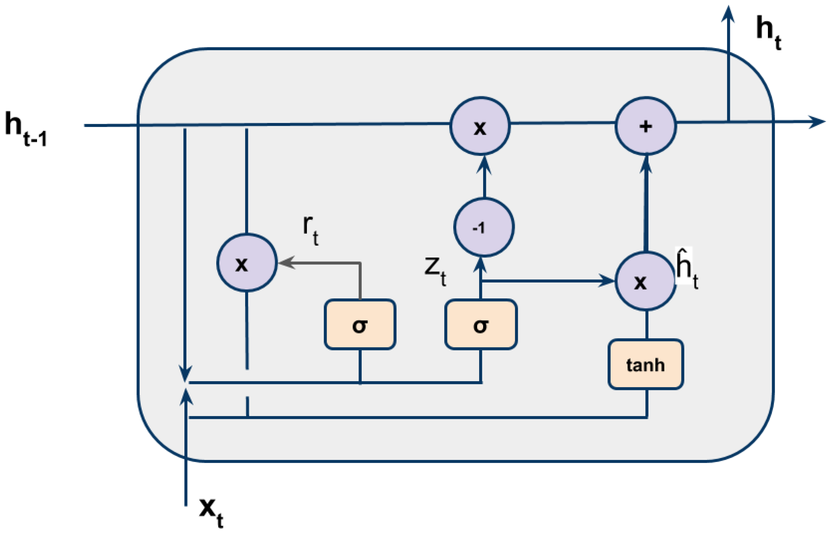
Cho et al. proposed GRU as a new type of recurrent unit that is much simpler to compute and implement compared to LSTM [34]. GRU, like the LSTM, consists of designing multiple cells that selectively remember important information and forget information that is considered irrelevant in the future [34]. The feedback loops of the Gated recurrent units can be interpreted as an unrolled network in time. The output of the cell from the earlier time period is used as an input to the cell state parallel to the current input so that the GRU is influenced by the current data along with previous data. This feature enables the model to remember the interesting patterns and is used to predict sequential data such as time-series data-sets over time. GRU contains only two gates: update and reset gates compared to input, output, and forget gates for LSTM. Thus, GRU presents a more compact representation of the current hidden state compared to LSTM [34]. An illustration of the GRU hidden activation function is presented in Figure 1. The update controls the amount of information from the previous state that will be carried over to the current hidden state. At the same time, the reset gate decides whether the new information will be added to the current state [34] or not or how much has to be passed. The cells within the GRU equations are as follows:

$$z_t=\sigma (W_z·\left[h_{t-1},x_t\right])$$

(1)

$$r_t=\sigma (W_r·\left[h_{t-1},x_t\right])$$

(2)

$$\widetilde{h_t}=tanh(W·\left[r_t·h_{t-1},x_t\right])$$

(3)

$$h_t=(1-z_t·h_{t-1}+z_t·h_t)$$

(4)

where $h_t$ is the output of GRU which is plays a role of being the forecasted output and an input to the next time-step and $W_z$, $W_r$, and W are the weights of each gate, x represents the current input, $\sigma$ is the sigmoid activation function. Both LSTM and GRU have different structures but use the same idea of using recurrent connections as one of the inputs and using the gates to modify the output.

GRU has shown to be one of the quite effective RNN techniques, due to its ability to learn and capture long-term dependencies and variable-length observations [35,36,37]. This property is especially helpful for time series data [38]. During the training phase, the GRU cells are trained to minimize the loss function using backpropagated weight adjusting through time. We evaluated the use of various cost functions in the network. We observed that minimizing the mean standard error generated the best forecast for the univariate approach, whereas using the mean absolute error for multivariate data resulted in a better prediction. To forecast the direct normal irradiance, historical solar irradiance from the previous time steps is used as the input. In our case, we consider DNI values from the daylight hours from the previous two days as the input to the model. In our experiments, all four networks contained the same features as Wojtkiewicz et al. [28]. The network includes ten cells for the univariate model with one layer, and three layers consisted of 30, 20, and 10 cells for multivariate models.

We investigated combinations of various configurable parameters including the type of optimizers and batch size. The Adam optimizer with a learning rate of 0.0001 with a batch size of 35 achieved the best performance in terms of the effectiveness of forecasting. The univariate models are trained for 100 epochs whereas the multivariate models are trained for 50 epochs. The total number of trainable parameters when using a GRU model is 25% less than those required for the LSTM [28].

2.2. Data Description

We collected real-world direct normal irradiance, weather data, and cloud cover from LRSS solar plant data that is publicly available. Irradiance and weather data were obtained from National Renewable Energy Laboratory’s Measurement, and Instrumentation Data Center for LRSS located near Denver, CO. DNI and weather features including zenith angle, humidity, dry bulb temperature, wind speed, and wind direction were extracted between August 2009 and January 2014 with 1-h granularity. These variables were chosen based on the Pearson correlation coefficients between DNI, and each of these variables indicates whether or not there is a robust linear relationship between DNI and each variable. Solar irradiance begins to increase at sunrise, reaches a maximum at solar noon, and returns to zero after sunset. The intensity varies throughout the year. The National Oceanic and Atmospheric Administration (NOAA) provides cloud cover data; we used the ISCCP HXG data with a resolution of 0.1 in angles of longitude and latitude for every three h, which is represented with 1 or 0 as the cloud covered or not, respectively. We calculate an average of pixels containing cloud cover to total nodes to determine the cloud activity and provided wind direction and wind speed of the location of interest. For our experiments, we used a net of nine nodes over the three pixels squared with the location of LRSS in the center of the grid. The direct normal irradiance, weather data, and cloud cover were aggregated by repeating the cloud cover ratios to match the solar irradiance and weather datasets. During the pre-processing step, a min-max normalization mapped the DNI, weather information, and cloud data to another map where all the variables were between 0 and 1.

2.3. Experimental Evaluation

To evaluate the capability of the proposed GRU-based RNN to forecast the irradiance values, we perform three sets of experiments. First, we assess the ability of the GRU to forecast the future values of GRU by using just the historical DNI values from LRSS. The model uses the irradiance from the previous two-day data to predict the direct normal irradiance for the hour ahead. We evaluated the performance of the models using the last 24, 48, and 72 h to forecast the next time step and configured that the previous two days daylight hours resulted in the best performance for both LSTM and GRU. To evaluate our proposed reframed networks, we took a set of three steps. In the first step, we trained a univariate GRU network comprised only of historical direct normal irradiance from LRSS. Our model reframed the last two days’ daylight hours data, to predict direct normal irradiance at the next hour. We tested the model for one, two, and three days (17 h per day) and found that using two-day data resulted in the best performance for both multivariate recurrent networks. Second: we design a Gated recurrent unit as our previous work that includes weather and cloud features like solar zenith angle, humidity, dry bulb temperature, wind direction, and wind speed along with cloud cover data to forecast the direct normal irradiance values for the next hour. In the multivariate model, we still consider the previous two days’ worth of historical data during the training phase of the process. Finally, we also evaluate the capability of the GRU to forecast DNI over multiple horizons for short term forecasting. This includes forecasting the solar irradiance for the next 15 min, 30 min, 1 h, 2 h, and 3 h respectively.

For each experiment, the data is split into 60 percent of initial data (44 months) for training, and the next 20 percent (12 months) validation, and the final 20 percent (12 months) testing to validate the model and compare the performance in terms of RMSE and MAPE metrics. Both Gated recurrent unit and Long-Short Term Memory networks are implemented using the TensorFlow and Keras libraries in Python.

3. Results

Table 1. Comparison of forecast errors at one time step ahead for one year of testing data.

Model	Univariate		Multivariate
			w/o Cloud Cover		w/o Wind Variables		All Variables
	RMSE ($\mathit{W}\mathbf{/}{\mathit{m}}^{\mathbf{2}}$)	MAPE $\mathbf{(}\mathbf{\%}\mathbf{)}$	RMSE ($\mathit{W}\mathbf{/}{\mathit{m}}^{\mathbf{2}}$)	MAPE $\mathbf{(}\mathbf{\%}\mathbf{)}$	RMSE ($\mathit{W}\mathbf{/}{\mathit{m}}^{\mathbf{2}}$)	MAPE $\mathbf{(}\mathbf{\%}\mathbf{)}$	RMSE ($\mathit{W}\mathbf{/}{\mathit{m}}^{\mathbf{2}}$)	MAPE $\mathbf{(}\mathbf{\%}\mathbf{)}$
LSTM	112.36	17.37	81.73	11.41	78.62	11.13	74.83	10.71
GRU	114.97	17.71	83.61	12.44	80.27	10.71	76.51	10.36

shows the results for one hour-ahead prediction of our experiments for the recurrent neural networks: univariate models, multivariate models without cloud cover and wind data, multivariate models with cloud cover and without wind data, and multivariate with all the features. We observe that including multivariate data improves the forecasting accuracy for both the LSTM and GRU, where the multivariate model using all the variables outperform the univariate models by at least 37.43% and 36.72% for LSTM and GRU respectively. The multivariate model, that includes all the variables, is much more accurate compared to multivariate models that exclude variables like cloud cover, wind direction, and wind speed. Thus ignoring cloud cover, wind direction, and wind speed would lead to less optimal forecasts, leading to higher errors in forecasted power generation capability of the solar farm. We also note that multivariate LSTM outperforms multivariate GRU for scenarios that include all the variables and also the model that excludes the cloud cover. We also evaluate the capability of both LSTM and GRU to forecast multiple time steps ahead when forecasting irradiance into the future. 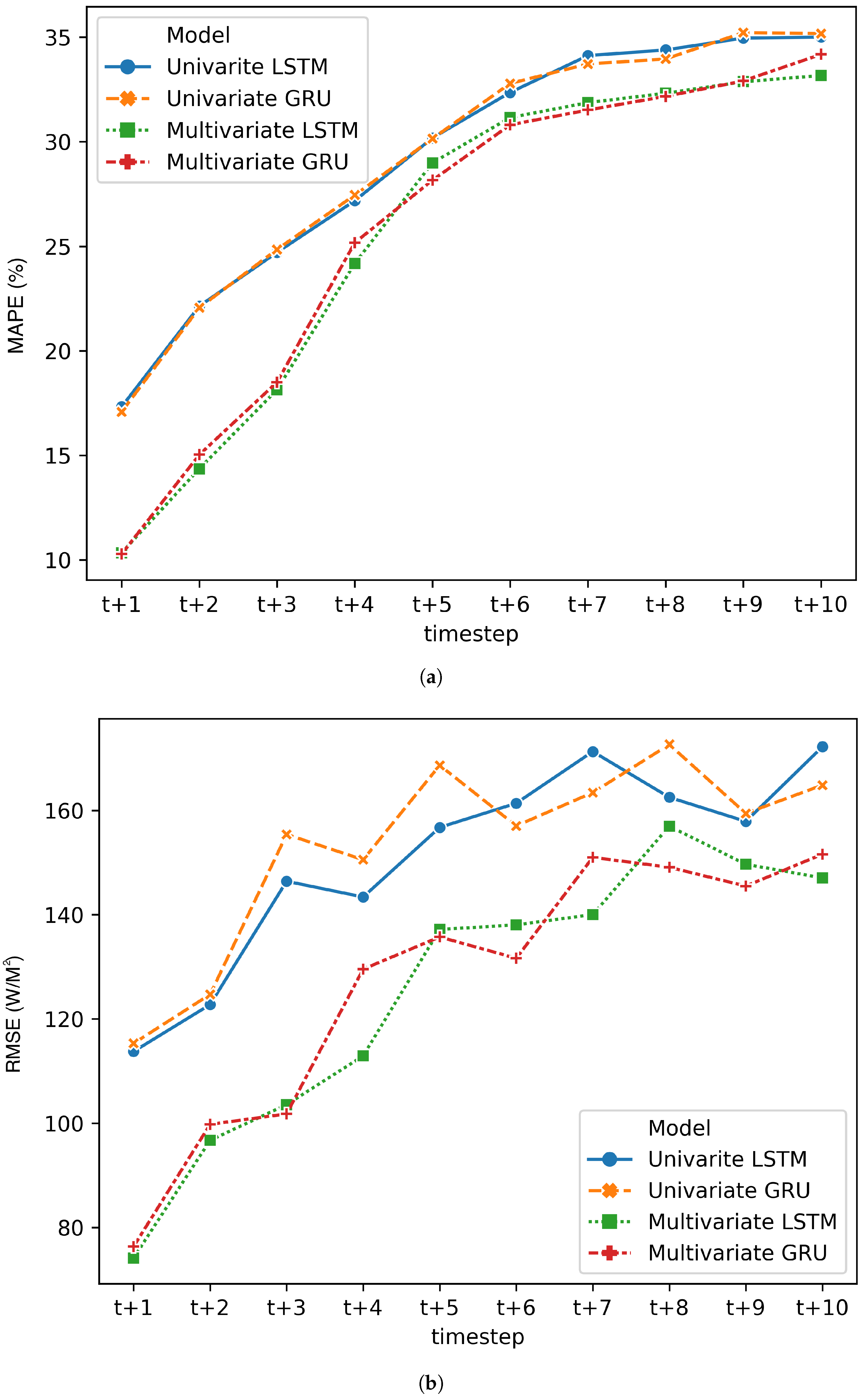Figure 2 presents the MAPE and RMSE for multi-step ahead forecasting for one step forward $(t+1)$ to 10 steps head $(t+10)$ forecast. The error increases for all the models as the number of steps increases with the univariate models performing worse than multivariate models in terms of MAPE. Still, the error trends between LSTM and GRU are virtually indistinguishable.

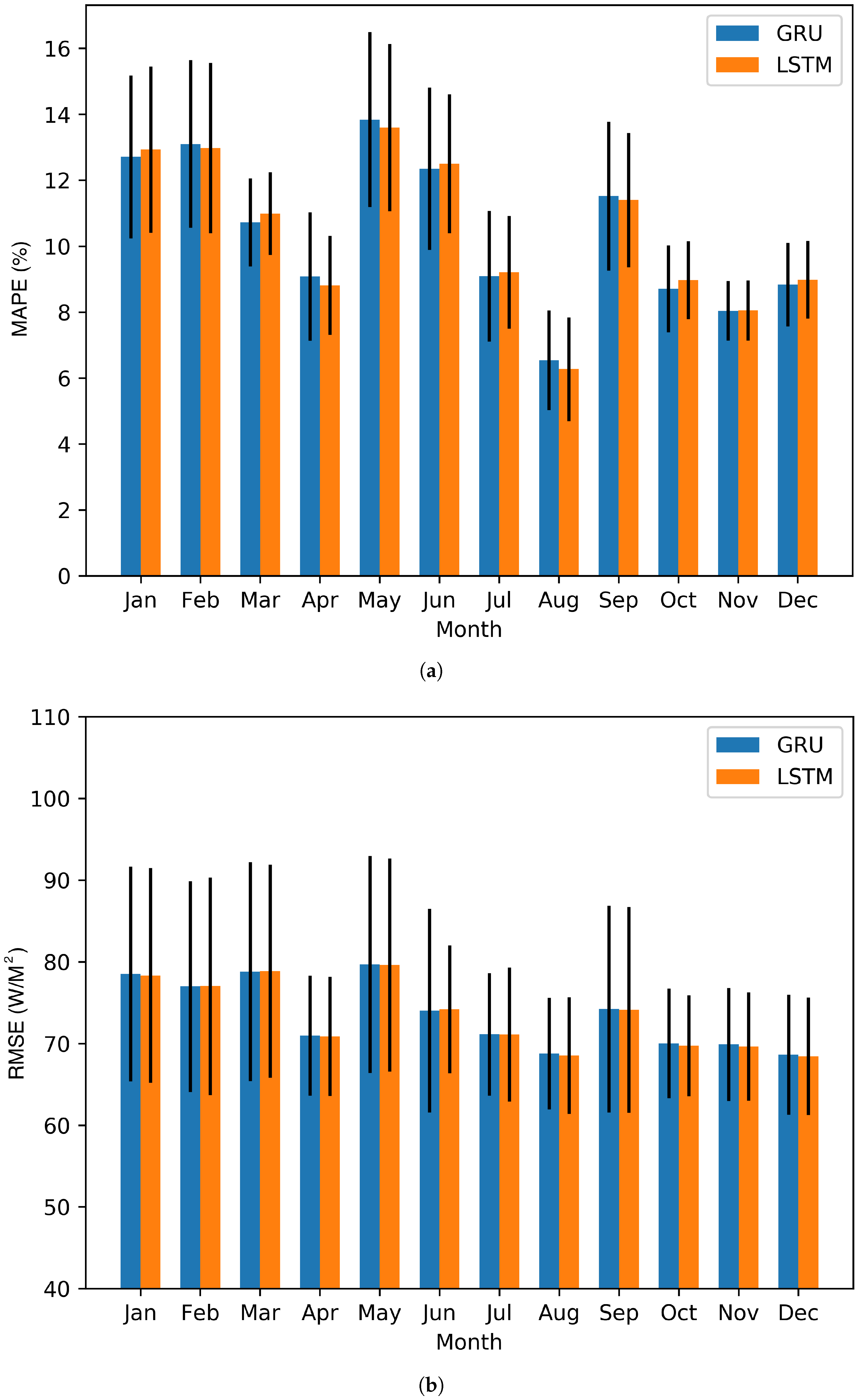
Figure 3 shows the average mean absolute percentage error (MAPE), and root mean squared error (RMSE) to forecast DNI including all the variables for all the months of the year in the testing set using multivariate Long-Short Term Memory and Gated Recurrent unit with all the variables included in the model. In six of the twelve months (April, July, August, October, November, and December), the MAPE values for both LSTM and GRU are less than 10 percent. Similarly, the RMSE values are less than 70 for 4 of the twelve months (i.e., August, October, November, and December). In both metrics, January, February, March, and June produced the highest amounts of error. Additionally, the standard errors are higher during these times of the year. 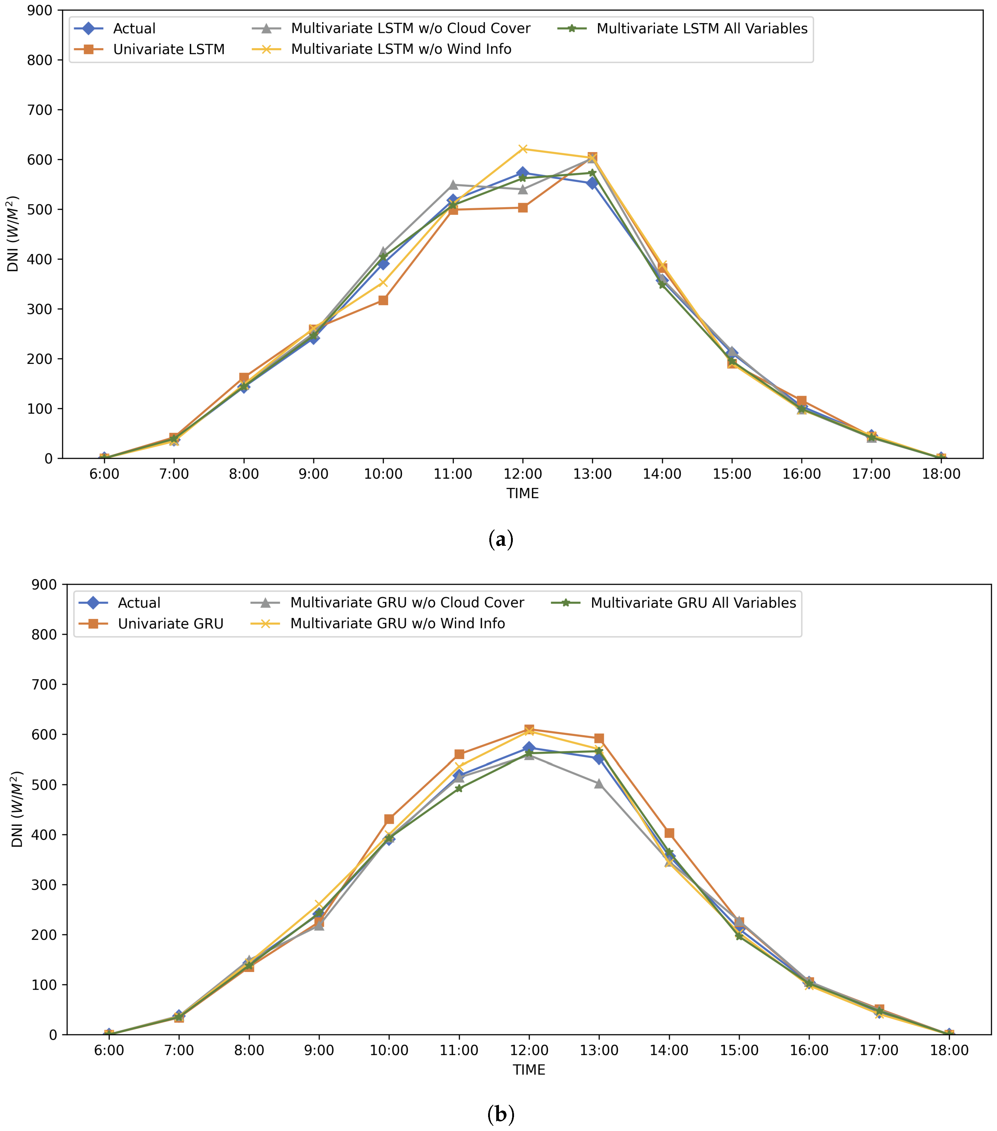Figure 4 illustrates the forecasted DNI using both LSTM and GRU based approaches during a clear day with no cloud cover for 1-h ahead forecasting. All the approaches are fairly accurate at forecasting DNI values in this setting. 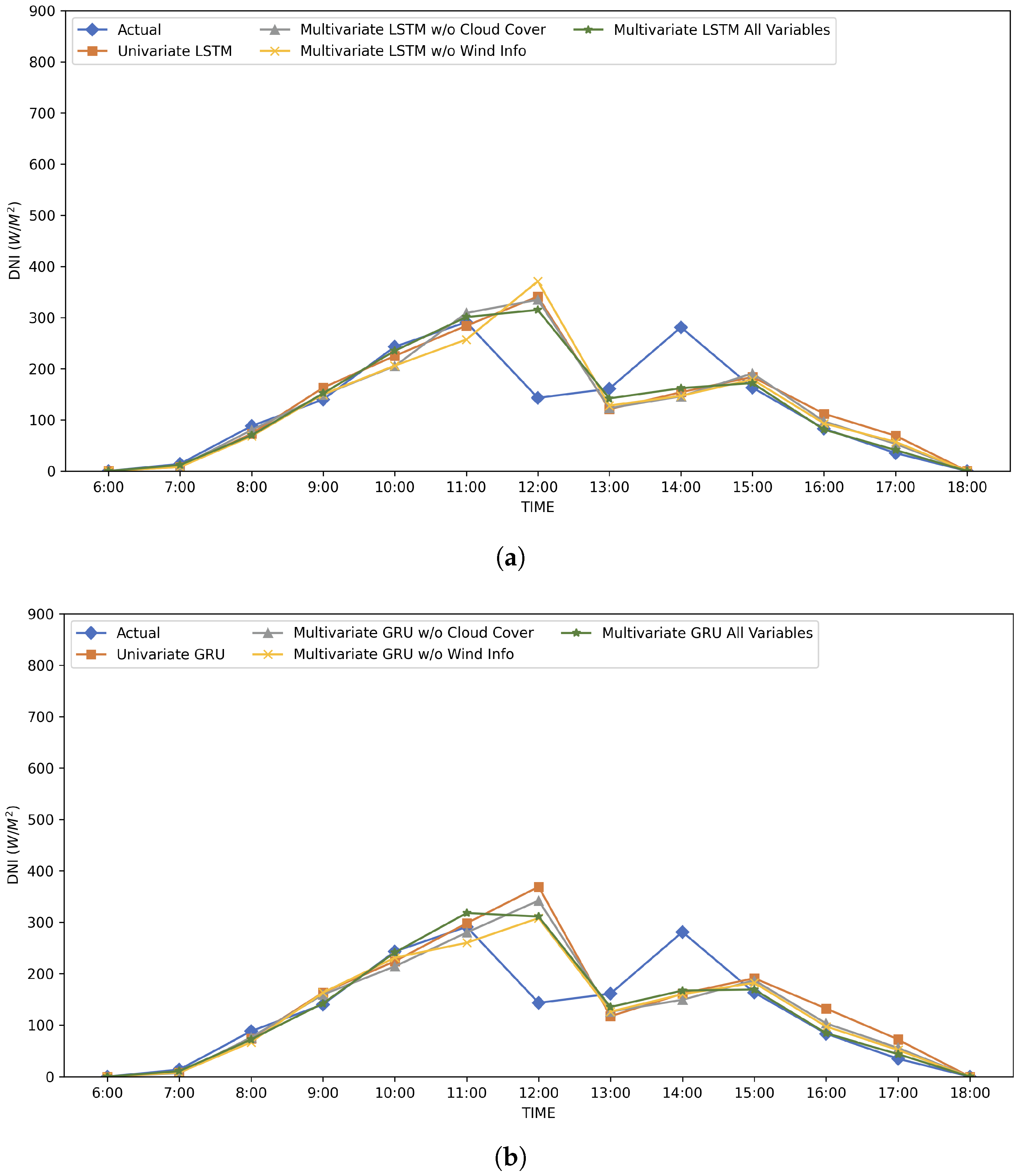However, as Figure 5 illustrates, these approaches are not as accurate for forecasting DNI on a cloudy day.

However, for various scenarios that include continuous, intermittent, and no cloud cover days, both LSTM and GRU predict similar results with the forecasts not being significantly different between the two models. In all these scenarios, the multivariate model outperforms the univariate model in terms of both MAPE and RMSE. Significant amounts of error were observed for the models when the model overestimated the solar irradiance after a substantial change in solar irradiance during the previous time period. The models assume that the next time period will follow the same pattern, which leads to an inaccurate forecast. DNI distribution during a typical day follows a bell curve with a gradual increase in DNI at sunrise, peak DNI in the afternoon, and a gradual decrease during the sunset. However, if the irradiance during the morning is inconsistent, the forecasted DNI for the rest of the day is much more inaccurate than reduced irradiance due to cloud cover during the afternoon or the evening. After a sudden change in direct normal irradiance, the models tend to overcorrect by decreasing the forecast solar irradiance in the following hour than accurately predicting the typical next prediction. These kinds of over corrections lead to a high MAPE and RMSE due to the reactivity of the models. The overall error is drastically higher on days where direct normal irradiance is stochastic due to cloud cover variations. The performance of these models can be improved by using a more granular cloud cover data [21].

We evaluated the capability of the proposed approaches to forecast DNI values over multiple time resolutions, and the MAPE and RMSE of various GRU models are presented in

Table 2. Comparison of MAPE for DNI forecasting at different time resolutions using various GRU based approaches.

		Multivariate
Time Resolution	Univariate	w/o Cloud Cover	w/o Wind Info	All Variables
15 min	26.75	19.81	17.42	12.14
30 min	22.31	16.18	13.67	10.56
1 h	17.08	12.4	10.97	10.28
2 h	16.31	12.31	11.31	10.17
3 h	15.95	12.52	11.92	10.84

and

Table 3. Comparison of RMSE for DNI forecasting at different time resolutions using various GRU based approaches.

		Multivariate
Time Resolution	Univariate	w/o Cloud Cover	w/o Wind Info	All Variables
15 min	143.57	86.13	83.16	78.15
30 min	128.12	84.53	84.19	77.32
1 h	114.97	83.61	80.27	76.51
2 h	104.83	84.21	79.54	75.84
3 h	94.17	82.95	79.31	78.31

. We did not notice any significant different between GRU and LSTM variants of this approach for multiple time resolutions. The training data required for each of these times are extended to include all the data that includes the previous 48 h of data. The number of historical irradiance values and weather attributes include $T=192$ for 15-min resolution prediction and $T=16$ for 3-h resolution prediction. The MAPE increases as the time resolution is increased, the variance of DNI and other exogenous variables increases with respect to the time resolutions. This variance leads to an increase on RMSE and MAPE for higher resolutions of data (2 and 3 h). In addition, the cloud cover data is only available every 3 h which leads to errors when used to forecast DNI at lower time resolutions.

The results show that both LSTM and GRU are capable of forecasting solar irradiance over multiple time steps. The MAPE and RMSE for both of these models are similar, with no significant difference between the forecasts generated by these two models. However, with the addition of more variables to the training data, the time is taken to train the models and forecast the predictions increases for both GRU and LSTM.

Table 4. Comparison of training and prediction time for LSTM and GRU.

Model	Training	Prediction
Univariate GRU	0.43 ± 0.03	1.21 ± 0.13
Univariate LSTM	0.52 ± 0.4	1.36 ± 0.21
Multivariate GRU w/o cloud	1.61 ± 0.07	4.13 ± 1.1
Multivariate LSTM w/o cloud	1.82 ± 0.14	4.18 ± 0.94
Multivariate GRU w/o wind	1.38 ± 0.11	3.73 ± 0.83
Multivariate LSTM w/o wind	1.47 ± 0.09	3.81 ± 1.02
Multivariate GRU All variables	2.34 ± 0.07	10.31 ± 2.14
Multivariate LSTM all variables	3.12 ± 0.09	10.43 ± 2.97

shows the training and prediction times for various experiments. An extensive hyper-parameter search is performed on the validation data during the training process to arrive at the final parameters of the model. The validation time is part of the training time for Deep neural networks. The experiments were conducted on a CentOS machine with a Intel Xeon E5 2600 v3 processor with 28 cores and a memory of 448 GB, no GPUs were used for this computation. The average training and testing time are computed over 20 executions on the same dataset. The time taken for multivariate models is almost six times longer than the univariate models. In all the experiments, the GRU variants of the models are consistently more computationally efficient in terms of training compared to LSTM models. This is primarily due to the number of trainable parameters for each of these models. The number of trainable parameters for the LSTM is almost 25% higher than the number of trainable parameters for the GRU.

4. Conclusions and Future Work

In this paper, we applied a GRU based approach for DNI forecasting that is more computationally efficient and is as accurate as LSTMs to forecast solar irradiance. We evaluated both univariate and multivariate GRU model configurations that were optimized to predict solar irradiance using historical irradiance values, weather information, and cloud cover information. These models were evaluated using the data extracted from the LRSS solar facility near Denver, Colorado. The proposed approach was compared against LSTM in terms of both accuracy of forecasts using MAPE and RMSE, as well as computation performance for training the model and predicting the value in the next time step. The proposed multivariate model outperforms the univariate model by 34.42% using RMSE and 41.31% using MAPE. We also evaluated the importance of including variables like cloud cover and wind direction and wind speed, which also seemed to improve the accuracy of forecasts by 23.32% and 8.91%, respectively. We also evaluated the performance of the multivariate GRU at forecasting multiple horizons of time intervals. Our analysis shows that the proposed multivariate GRU is computationally efficient compared to traditional LSTM models for forecasting irradiance values with no significant effect on the accuracy of forecasts.

We plan to extend the current work by improving the quality of data used for forecasting. This includes using a finer level of granularity of cloud cover data as well as incorporating more features on cloud cover such as aerosol content etc. Additional improvements to the models include adapting a weather forecast model in addition to the historical weather prediction model that can predict further weather forecasts that can be used to improve the quality of irradiance forecasts. Our results indicate that the model over-corrects when there is a sudden change in the irradiance values due to changes in the solar facility’s local environment. We would like to extend our work to include a concept drift-based approach that can predict solar irradiance for changes in various variables, which can then be used to build an ensemble approach for forecasting.