DPsim—Advancements in Power Electronics Modelling Using Shifted Frequency Analysis and in Real-Time Simulation Capability by Parallelization

Abstract

Real-time simulation is an increasingly popular tool for product development and research in power systems. However, commercial simulators are still quite exclusive due to their costs and they face problems in bridging the gap between two common types of power system simulation, conventional phasor based, and electromagnetic transient simulation. This work describes recent improvements to the open source real-time simulator DPsim to address increasingly important use cases that involve power electronics that are connected to the electrical grid and increasing grid sizes. New power electronic models have been developed and integrated into the DPsim simulator together with techniques to decouple the system solution, which facilitate parallelization. The results show that the dynamic phasors in DPsim, which result from shifted frequency analysis, allow the user to combine the characteristics of conventional phasor and electromagnetic transient simulation. Besides, simulation speed up techniques that are known from the electromagnetic domain and new techniques, specific to dynamic phasors, significantly improve the performance. It demonstrates the advantages of dynamic phasor simulation for future power systems and the applicability of this concept to large scale scenarios.

1. Introduction

Real-time simulation is increasingly applied in power systems for testing new components and algorithms. However, power system simulators that are capable of real-time execution are still not accessible for many researchers and product developers. One reason for the high cost of real-time power system simulators is the customized hardware platform that is usually required. Early real-time simulators used special purpose processors, e.g., digital signal processors (DSP). Today, general purpose processors are commonly employed as the core computing unit but often in combination with additional hardware, such as a customized backplane to interconnect computing units or field-programmable gate arrays (FPGAs) [1]. The use of FPGAs as main computing unit is gaining traction with the advent of power electronics simulation. While this approach is only adopted by few commercial manufacturers, there are many examples of FPGA driven real-time simulators built by researchers [2,3,4,5]. An interesting alternative direction is presented in [6], where real-time simulation is conducted on a small low cost device. However, [6] is based on quasi-static assumptions, whereas the aim of this work is a more detailed represention of dynamics. DPsim (https://github.com/dpsim-simulator), the simulator employed and extended in the frame of this work, is capable of running real-time simulation on commercial off-the-shelf hardware without neglecting electromagnetic dynamics.

This is possible due to shifted frequency analysis (SFA) [7], which enables larger simulation time steps for the same simulated signal frequencies as compared to electromagnetic-transient (EMT) simulations. Larger time steps facilitate the simulation on standard hardware and in large scale because the requirements on computational speed can be relaxed. The SFA approach intends to bridge the gap between EMT and conventional phasor simulation in terms of accuracy. Applying SFA on a real signal results in one or many time-varying phasors, which are often denoted as dynamic phasors (DP).

DPsim is not the first simulator that is based on this approach. Previous developments of SFA or dynamic phasor based simulators are described in [8,9,10]. In contrast to DPsim, these simulators do not seem to aim at real-time execution and related topics, such as parallelization, to speed up the simulation. As described in this paper, DPsim supports the simulation of higher order harmonics to accurately represent switching power electronics. The other simulators only focus on the fundamental system frequency phasor or lower order harmonics resulting from the dq0 transform in combination with unbalanced conditions as in [9]. While previous SFA models implemented in DPsim have not required an approximation of the phasors using Fourier analysis, the detailed inverter model results presented in the following rely on it to compute the phasor values for each time step. This approach is based on the generalized state space averaging method that is explained in [11] and harmonic analysis of the inverter circuit [12].

Most importantly, DPsim is developed as open source in contrast to the aforementioned projects. It allows the user not only to compare and validate against other solutions, but also to understand the implementation in detail. Besides, DPsim supports a faster transition from offline testing to real-time execution, since the same software and hardware system is used in both cases.

The dynamic phasor approach is not only used in the development of simulators, but also for the interconnection of real-time simulators, especially if there is a considerable distance between these simulators. This idea is presented in [13], where several EMT simulators are interconnected via a dynamic phasor interface that is based on the VILLAS software project [14].

DPsim was first introduced by Mirz et al. [15], which describes the main software components and demonstrates the real-time capability of the simulator for different system sizes. It integrates the VILLAS project to facilitate the exchange of simulation data in real-time taking advantage of the vast collection of protocols supported by VILLAS. A possible simulation framework architecture that is based on DPsim and VILLAS is described in [16]. Although DPsim primarily targets the dynamic phasor domain, the solver also supports EMT and quasi-static simulations. The main input format for network description is the IEC 61970 CIM XML-RDF format, which is imported by using the CIM++ project [17]. A more detailed overview of the features of DPsim can be found in [15]. The aim of DPsim is to support real-time simulation with time steps in the range from 10 $\mathsf{\mu }$s to several $\mathrm{ms}$. Due to the frequency shift applied when computing dynamic phasors, the maximum frequency of simulated signals is not limited by the simulation time step.

Until now, DPsim only supported traditional power system components, such as synchronous generators, lines, and transformers. Here, we describe two new power electronics models and one new parallelization method, which were implemented in DPsim. First, an averaged inverter model is presented and how an associated dq0 state-space controller can be integrated into the simulation. The second model is more detailed and it extends the averaged model by harmonics resulting from switches. A new method for the DPsim solver is demonstrated that ensures real-time capability for such an inverter model with a large number of harmonics. Besides, the explanation of the subsystem decoupling using the transmission line method briefly presented in [15] is extended by a description on how the line model is adapted for SFA.

Section 2 briefly summarizes SFA and how it computes dynamic phasor variables. A detailed description of the component models and methods used to obtain the simulation results can be found in Section 3. Section 4 and Section 5 present and discuss the results.

2. Theoretical Background

The basic concept of SFA, constructing a frequency shifted complex representation of a real valued physical signal, is also established in other domains, e.g., microwave and communications engineering [18,19]. In these domains, the concept is commonly denoted as baseband representation or complex envelope. The research reported in the power engineering domain can be roughly divided into two categories, Hilbert or Fourier based. The phasor representation can be derived from the analytical signal constructed from the Hilbert transform or by applying Fourier transform.

The Hilbert based approach is commonly applied in the power system domain, where it is referred to as envelope waveforms [8], dynamic phasors [20], or SFA [21]. The second approach relies on the Fourier transform to approximate a physical signal by a series of Fourier coefficients and it has been developed in the power electronics domain as generalized state space averaging [11]. In more recent publications, SFA and dynamic phasors have been associated to the Hilbert and Fourier based approach [7,22]. In the following, the variables that result from SFA are denoted as dynamic phasors, regardless of which one of the approaches is used.

A dynamic phasor can be considered as a projection of a signal defined as a function over time onto the time-frequency plane. Dynamic phasors are not a spectral representation over an infinite time interval, which would eliminate the time dependency as in a frequency spectrum. Instead, dynamic phasors depend on both time and frequency.

The Hilbert approach is based on the analytical signal, which can be derived from a real signal by extending it with an imaginary part that is equal to the Hilbert transform of the original signal (1).

$$\mathcal{A}\left\{s\right(t\left)\right\}=s\left(t\right)+j\mathcal{H}\left\{s\right(t\left)\right\}$$

(1)

Applying (1) to a bandpass signal $s_{bp}\left(t\right)=A\left(t\right)cos({\omega }_{c}t+\theta \left(t\right))$, results in the analytical representation corresponding to a generic bandpass signal:

$$\begin{array}{cc}\hfill \mathcal{A}\left\{s_{bp}\left(t\right)\right\}& =s_{bp}\left(t\right)+j\mathcal{H}\left\{s_{bp}\left(t\right)\right\}\hfill \\ \hfill & =s_{bp,I}\left(t\right)cos\left({\omega }_{c}t\right)-s_{bp,Q}\left(t\right)sin\left({\omega }_{c}t\right)+j(s_{bp,I}\left(t\right)sin\left({\omega }_{c}t\right)+s_{bp,Q}\left(t\right)cos\left({\omega }_{c}t\right))\hfill \\ \hfill & =(s_{bp,I}\left(t\right)+j{s}_{bp,Q}\left(t\right))(cos\left({\omega }_{c}t\right)+jsin\left({\omega }_{c}t\right))\hfill \\ \hfill & =\langle s_{bp}\rangle \left(t\right)e^{j{\omega }_{c}t}\hfill \end{array}$$

(2)

with the in-phase component $s_{bp,I}\left(t\right)=A\left(t\right)cos\left(\theta \left(t\right)\right)$ and the quadrature component $s_{bp,Q}\left(t\right)=A\left(t\right)sin\left(\theta \left(t\right)\right)$. In order to calculate the dynamic phasor from the analytical signal, it is shifted by the center frequency ${\omega }_c$ (3).

$$\langle s\rangle \left(t\right)=\mathcal{A}\left\{s\left(t\right)\right\}{e}^{-j{\omega }_{c}t}$$

(3)

The Fourier transform is common in the power electronics domain, because it can be applied to monocomponent as well as multicomponent signals, where more than one frequency band are of interest. The disadvantage of the Fourier transform for time-frequency analysis is that it suffers from the uncertainty principle. Time and frequency resolution cannot be increased arbitrarily at the same time, which complicates the calculation of accurate dynamic phasors. Each phasor is approximated by a Fourier coefficient that is dynamically changing over time. The time dependency of the Fourier coefficients results from the sliding Fourier transform. Applying a sliding observation window of time T, the time dependent Fourier coefficients are expressed by the transform (4), where ${\omega }_c$ is the fundamental frequency.

$${\langle s\rangle }_k\left(t\right)=\frac{1}{T}{\int }_{t-T}^{t}s\left(\tau \right)·e^{-jk{\omega }_c\tau }d\tau$$

(4)

An accuracy analysis of the basic approach used in the DPsim solver, which is the combination of frequency shifted phasor variables and the trapezoidal rule as discretization method, can be found in [8].

3. Models and Methods

The following sections describe, in detail, the models simulated in Section 4: averaged inverter, inverter with harmonics, and transmission line. The last section explains how the simulation can be more efficiently parallelized in the case of detailed power electronics models. First, the solution process of DPsim is reviewed, including the transmission line method (TLM) for subsystem decoupling. Subsequently, the process is extended with a method to split the network not only between nodes, but also across frequencies to compensate for the increased number of equations when simulating the inverter model with harmonics.

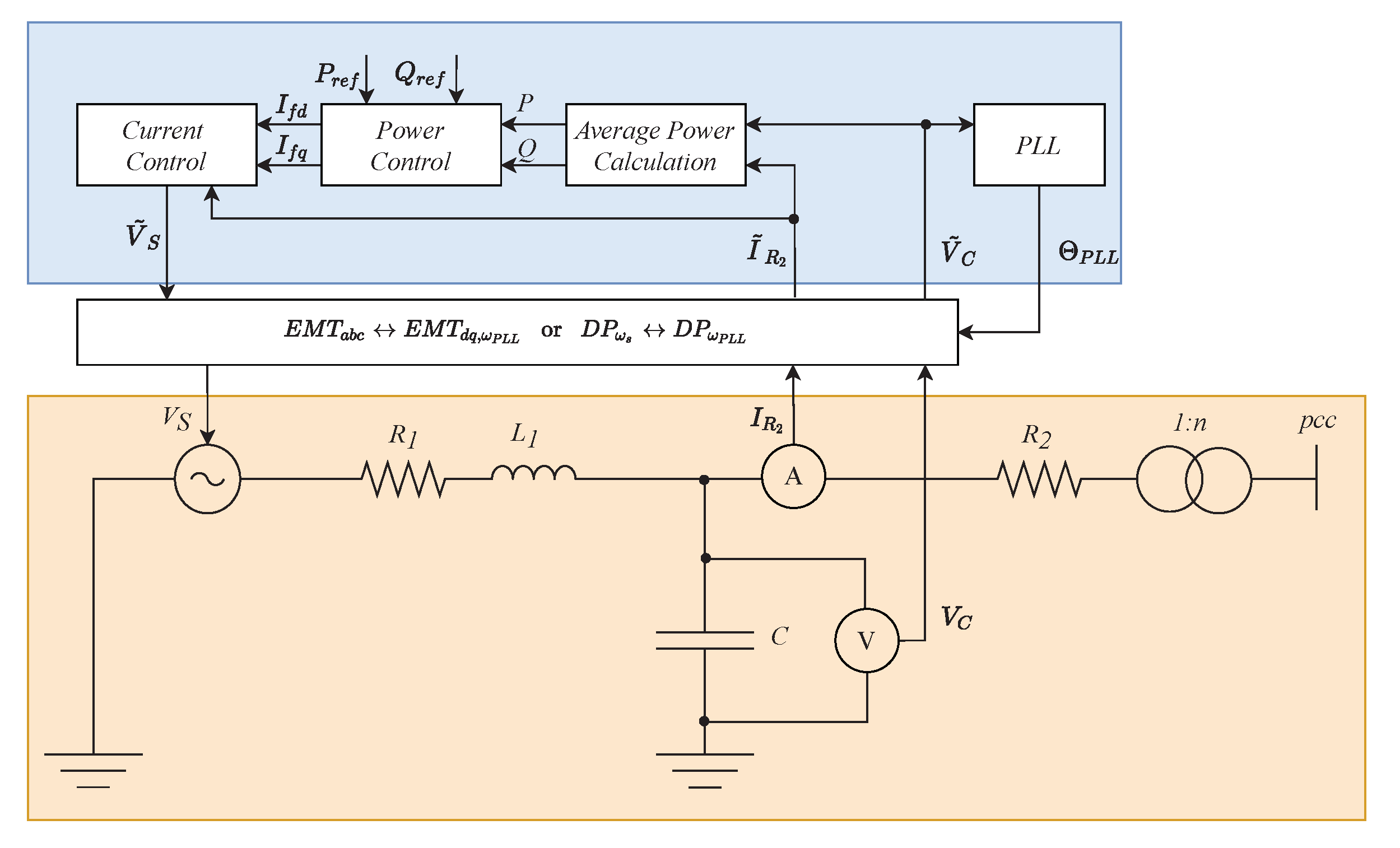
3.1. Averaged Inverter Model with Controls

The averaged model with controls encompasses three kinds of components: electrical components, control components, and interface components connecting the former two. The averaged inverter model is applied in DPsim for both types of simulations DP and EMT, see Section 4.1. This section is focused on the description of how the inverter’s control, which is modelled in state space, is interfaced with the inverter’s and grid’s electrical components in the case of DP and EMT simulation.

The inverter is modelled as Voltage Source Inverter (VSI), see Figure 1. Accordingly, a controlled voltage source represents the inverter’s output based on an averaged switching model. Besides, the inverter model includes an LC filter as output filter, which is composed of two resistors, an inductor and a capacitor. The inverter model operates at low voltage (LV) level and the grid operates at medium voltage (MV) level. Therefore, the inverter includes a step-up transformer for connection to the MV grid. The chosen parameters are listed in

Table 1. Averaged inverter example parameters.

Attribute	Value
$R_1$	$0.1$$\mathsf{\Omega }$
$L_1$	2 $\mathrm{m}$$\mathrm{H}$
C	$789.3$$\mathsf{\mu }$$\mathrm{F}$
$R_2$	$0.1$$\mathsf{\Omega }$
$L_{transformer}$	$928.3$$\mathrm{m}$$\mathrm{H}$

.

As mentioned in Section 3.4, DPsim follows the modified nodal analysis approach in order to solve the electrical network. Accordingly, the inverter’s electrical components that are mentioned above are integrated into the system solution by stamping their contributions into system matrix and source vector. The dynamic behaviour of the components is taken into account by means of the components’ DC equivalents [23]. Depending on the type of simulation, the DC equivalents represent the models either in the DP or the EMT domain.

The inverter’s control is modelled in state space and it enables an operation of the inverter in grid feeding mode [24]. The control aims at injecting active and reactive power according to specified reference values. The actual power feed-in is determined through an average power calculation, including a low-pass filter. The power calculation serves as input to power and current control loop, which are both implemented as PI controllers and that finally provide the voltage set-point for the controlled voltage source. As common in the field of control engineering, the inverter’s control is modelled in state space. The state space model employs quantities represented in the inverter’s local dq reference frame, which rotates with the frequency measured by a phase-locked-loop (PLL). The interface connecting the electrical model with the controller’s model in state space depends on the domain in which the electrical simulation is performed.

In case of an EMT simulation, the quantities are represented with respect to a stationary reference frame. The grid quantities are represented in DPsim as real-valued phase-to-ground peak quantities $x=\begin{array}{ccc}[{\widehat{x}}_a& {\widehat{x}}_b& {\widehat{x}}_c]\end{array}$. To obtain the quantities in the inverter’s local reference frame rotating with ${\omega }_{PLL}$, they are transformed by means of the power-invariant dq transformation, according to

$$\begin{array}{c}\hfill \left[\begin{array}{c}{x}_{d,{\omega }_{PLL}}\\ x_{q,{\omega }_{PLL}}\end{array}\right]=\underset{T_{dq,{\theta }_{PLL}}}{\underbrace{\sqrt{\frac{2}{3}}\left[\begin{array}{ccc}cos\left({\theta }_{PLL}\right)& cos({\theta }_{PLL}-\frac{2\pi }{3})& cos({\theta }_{PLL}+\frac{2\pi }{3})\\ -sin\left({\theta }_{PLL}\right)& -sin({\theta }_{PLL}-\frac{2\pi }{3})& -sin({\theta }_{PLL}+\frac{2\pi }{3})\end{array}\right]}}\left[\begin{array}{c}{\widehat{x}}_a\\ {\widehat{x}}_b\\ {\widehat{x}}_c\end{array}\right].\end{array}$$

(5)

This means that the inverter’s input variables $v_C$ and $i_{R_2}$, see Figure 1, are transformed to ${\tilde{v}}_C$ and ${\tilde{i}}_{R_2}$ according to

$$\begin{array}{c}\hfill {\tilde{v}}_C=\left[\begin{array}{c}{v}_{C,d,{\omega }_{PLL}}\\ v_{C,q,{\omega }_{PLL}}\end{array}\right]=T_{dq,{\theta }_{PLL}}\underset{v_C}{\underbrace{\left[\begin{array}{c}{\widehat{v}}_{C,a}\\ {\widehat{v}}_{C,b}\\ {\widehat{v}}_{C,c}\end{array}\right]}}\end{array}$$

(6)

$$\begin{array}{c}\hfill {\tilde{i}}_{R_2}=\left[\begin{array}{c}{i}_{R_2,d,{\omega }_{PLL}}\\ i_{R_2,q,{\omega }_{PLL}}\end{array}\right]=T_{dq,{\theta }_{PLL}}\underset{i_{R_2}}{\underbrace{\left[\begin{array}{c}{\widehat{i}}_{R_2,a}\\ {\widehat{i}}_{R_2,b}\\ {\widehat{i}}_{R_2,c}\end{array}\right]}}.\end{array}$$

(7)

The inverter’s controllers deliver as output the quantities in the local reference frame, which are then transformed back to the grid’s stationary frame by means of the inverse dq transformation

$$\begin{array}{c}\hfill \left[\begin{array}{c}{\widehat{x}}_a\\ {\widehat{x}}_b\\ {\widehat{x}}_c\end{array}\right]=\underset{T_{dq,{\theta }_{PLL}}^{-1}}{\underbrace{\sqrt{\frac{2}{3}}\left[\begin{array}{cc}cos\left({\theta }_{PLL}\right)& -sin\left({\theta }_{PLL}\right)\\ cos({\theta }_{PLL}-\frac{2\pi }{3})& -sin({\theta }_{PLL}-\frac{2\pi }{3})\\ cos({\theta }_{PLL}+\frac{2\pi }{3})& -sin({\theta }_{PLL}+\frac{2\pi }{3})\end{array}\right]}}\left[\begin{array}{c}{x}_{d,{\omega }_{PLL}}\\ x_{q,{\omega }_{PLL}}\end{array}\right].\end{array}$$

(8)

Correspondingly, the controller’s output voltage $v_S$ is considered in the grid solution after the back transformation of ${\tilde{v}}_S$, according to

$$\begin{array}{c}\hfill v_S=\left[\begin{array}{c}{\widehat{v}}_{S,a}\\ {\widehat{v}}_{S,b}\\ {\widehat{v}}_{S,c}\end{array}\right]=T_{dq,{\theta }_{PLL}}^{-1}\underset{{\tilde{v}}_S}{\underbrace{\left[\begin{array}{c}{v}_{S,d,{\omega }_{PLL}}\\ v_{S,q,{\omega }_{PLL}}\end{array}\right]}}.\end{array}$$

(9)

In case of a DP simulation, DPsim uses complex phase-to-phase RMS quantities denoted as ${\langle x\rangle }_{{\omega }_c}=\begin{array}{cc}[{\langle x\rangle }_{{\omega }_c,re}& {\langle x\rangle }_{{\omega }_c,im}]\end{array}$ following Equation (2). In contrast to the next section, we consider at this point exclusively the first order DP at center frequency ${\omega }_c$. The grid quantities have the grid’s synchronous frequency ${\omega }_S$ as center frequency, which is usually equal to 50 or 60 Hz. Thus, the original EMT quantities are related to the DP grid quantities by

$$\begin{array}{c}\hfill \left[\begin{array}{c}{\widehat{x}}_a\\ {\widehat{x}}_b\\ {\widehat{x}}_c\end{array}\right]=Re\left\{\sqrt{\frac{2}{3}}{\langle x\rangle }_{{\omega }_S}{e}^{j{\theta }_S}\left[\begin{array}{c}1\\ e^{-j\frac{2\pi }{3}}\\ e^{j\frac{2\pi }{3}}\end{array}\right]\right\}.\end{array}$$

(10)

with ${\theta }_S={\omega }_{S}t$. Instead, the inverter’s input and output quantities imply the local frequency ${\omega }_{PLL}$ as center frequency, which is defined through the PLL’s angle ${\theta }_{PLL}$. Accordingly, the inverter’s quantities are related to the original EMT quantities by

$$\begin{array}{c}\hfill \left[\begin{array}{c}{\widehat{x}}_a\\ {\widehat{x}}_b\\ {\widehat{x}}_c\end{array}\right]=Re\left\{\sqrt{\frac{2}{3}}{\langle x\rangle }_{{\omega }_{PLL}}{e}^{j{\theta }_{PLL}}\left[\begin{array}{c}1\\ e^{-j\frac{2\pi }{3}}\\ e^{j\frac{2\pi }{3}}\end{array}\right]\right\}\end{array}$$

(11)

Comparing Equations (10) and (11) yields the following relationship between the DPs with two different center frequencies

$$\begin{array}{c}\hfill {\langle x\rangle }_{{\omega }_{PLL}}={\langle x\rangle }_{{\omega }_S}{e}^{j({\theta }_S-{\theta }_{PLL})}.\end{array}$$

(12)

Thus, the transformation from DPs with the grid’s synchronous frequency ${\omega }_S$ as center frequency to DPs with the inverter’s frequency ${\omega }_{PLL}$ as center frequency looks as follows

$$\begin{array}{c}\hfill \left[\begin{array}{c}{\langle x\rangle }_{{\omega }_{PLL},re}\\ {\langle x\rangle }_{{\omega }_{PLL},im}\end{array}\right]=\underset{=:T_{DP,{\theta }_S-{\theta }_{PLL}}}{\underbrace{\left[\begin{array}{cc}cos({\theta }_S-{\theta }_{PLL})& -sin({\theta }_S-{\theta }_{PLL})\\ sin({\theta }_S-{\theta }_{PLL})& cos({\theta }_S-{\theta }_{PLL})\end{array}\right]}}\left[\begin{array}{c}{\langle x\rangle }_{{\omega }_S,re}\\ {\langle x\rangle }_{{\omega }_S,im}\end{array}\right].\end{array}$$

(13)

Accordingly, the inverter’s input quantities can be obtained from

$$\begin{array}{c}\hfill {\tilde{v}}_C=\left[\begin{array}{c}{\langle v_C\rangle }_{{\omega }_{PLL},re}\\ {\langle v_C\rangle }_{{\omega }_{PLL},im}\end{array}\right]=T_{DP,{\theta }_S-{\theta }_{PLL}}\underset{v_C}{\underbrace{\left[\begin{array}{c}{\langle v_C\rangle }_{{\omega }_S,re}\\ {\langle v_C\rangle }_{{\omega }_S,im}\end{array}\right]}}\end{array}$$

(14)

$$\begin{array}{c}\hfill {\tilde{i}}_{R_2}=\left[\begin{array}{c}{\langle i_{R_2}\rangle }_{{\omega }_{PLL},re}\\ {\langle i_{R_2}\rangle }_{{\omega }_{PLL},im}\end{array}\right]=T_{DP,{\theta }_S-{\theta }_{PLL}}\underset{i_{R_2}}{\underbrace{\left[\begin{array}{c}{\langle i_{R_2}\rangle }_{{\omega }_S,re}\\ {\langle i_{R_2}\rangle }_{{\omega }_S,im}\end{array}\right]}}.\end{array}$$

(15)

Besides, the inverter’s output voltage is transformed back according to

$$\begin{array}{c}\hfill v_S=\left[\begin{array}{c}{\langle v_S\rangle }_{{\omega }_S,re}\\ {\langle v_S\rangle }_{{\omega }_S,im}\end{array}\right]=T_{DP,{\theta }_{PLL}-{\theta }_S}\underset{{\tilde{v}}_S}{\underbrace{\left[\begin{array}{c}{\langle v_S\rangle }_{{\omega }_{PLL},re}\\ {\langle v_S\rangle }_{{\omega }_{PLL},im}\end{array}\right]}}.\end{array}$$

(16)

It can be noted that the transformation matrix in Equation (8), which links the inverter’s dq variables $\begin{array}{cc}[x_{d,{\omega }_{PLL}}& x_{q,{\omega }_{PLL}}]\end{array}$ with the original EMT variables, is the same as the transformation matrix obtained when resolving Equation (11), which links the inverter’s DP variables $\begin{array}{cc}[{\langle x\rangle }_{{\omega }_{PLL},re}& {\langle x\rangle }_{{\omega }_{PLL},im}]\end{array}$ with the original EMT variables. That is, the described interfaces ensure that, from a theoretical perspective, the inverter model in state space operates on the same quantities for EMT and DP simulation, while from a simulation perspective these quantities can significantly differ in terms of accuracy, as shown in Section 4.1.

Using these interfaces, other state space controllers can be integrated into DPsim in the same way. Control models operating on dq variables with respect to a local reference frame can be easily integrated into DPsim and applied in both EMT and DP simulations.

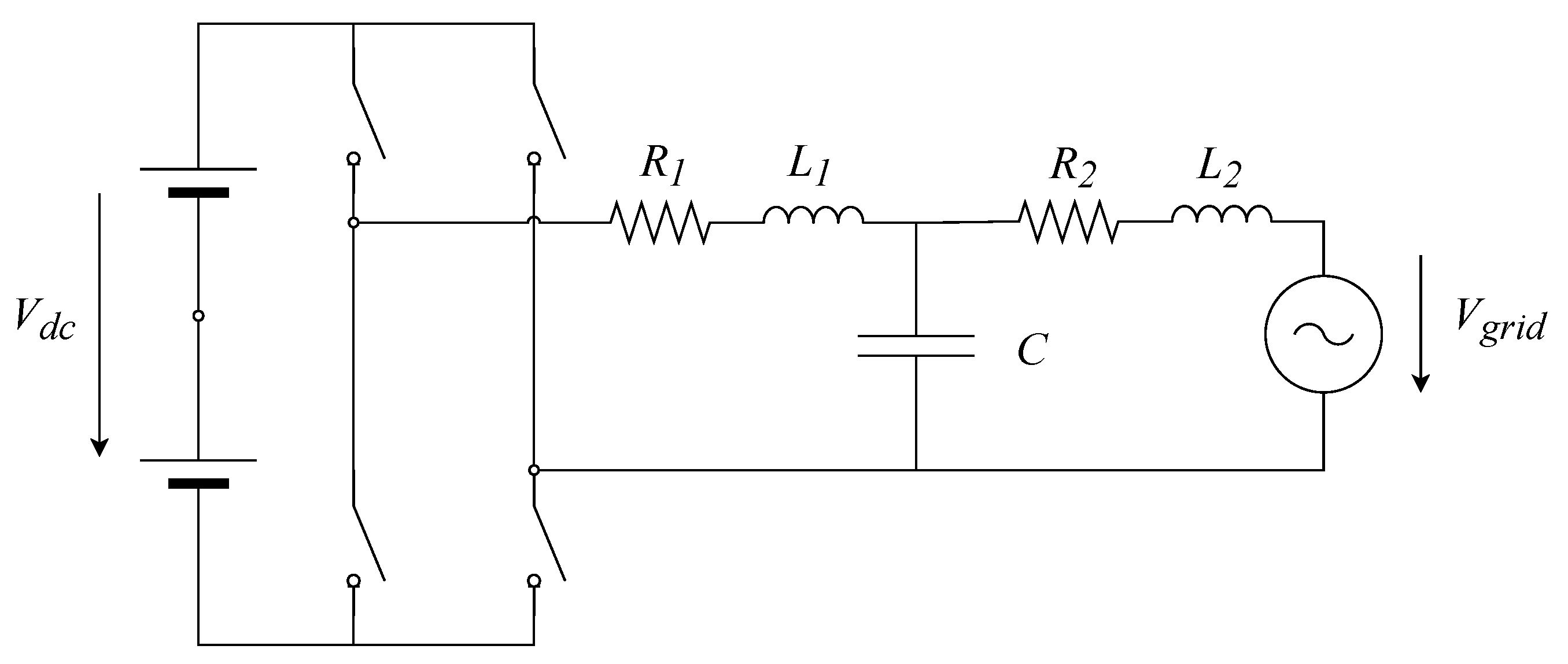
3.2. Inverter Model Including Harmonics

Here, harmonic analysis is applied to determine the dynamic phasor quantities injected into the grid by a unipolar single-phase full-bridge voltage source inverter. The harmonic frequency content of power electronics topologies could also be determined by a Fast Fourier Transform (FFT) of the electromagnetic transient waveform, which reduces the mathematical effort, but it requires extra computing capacity. Instead, the harmonic components of the PWM waveform can be computed directly, which is more precise [12].

In the following, it is assumed that the PWM signal is generated by comparing a triangular carrier signal and a reference signal of the form (17). The reference signal is defined by the nominal grid frequency ${\omega }_0$, the modulation index $M_r$, and the reference signal phase $\phi$.

$$s_{ref}\left(t\right)=M_{r}cos({\omega }_{0}t+\phi )$$

(17)

Applying double Fourier integral analysis, as explained in [12], the resulting PWM waveform can be expressed in terms of Fourier coefficients (18). With respect to [12], the following equations have been reformulated in a way that allows fewer evaluations of the series term, which facilitates efficient implementation. Besides, a phase angle of the reference signal different from zero is considered. In this case, double edge natural sampling is assumed for the PWM signal. This means that the carrier signal is triangular instead of sawtooth (trailing edge), and switching is initiated whenever the carrier and reference signal cross.

$$\begin{array}{cc}\hfill v_{inv}\left(t\right)& =A_{nd,1}cos({\omega }_{0}t+\phi )\hfill \\ \hfill & +\frac{4V_{in}}{\pi }\sum _{m=2,4,...}^{\infty }\sum _{n=\pm 1,\pm 3,...}^{\infty }{A}_{nd,2}(m,n)cos(m{\omega }_{sw}t+n({\omega }_{0}t+\phi ))\hfill \\ \hfill A_{nd,1}& =M_r{V}_{in}\hfill \\ \hfill A_{nd,2}(m,n)& =\frac{J_n(m{M}_r\pi /2)}{m}sin\left(\frac{(m+n)\pi }{2}\right)\hfill \end{array}$$

(18)

$J_n$ is the Bessel function defined as:

$$J_n\left(x\right)=\sum _{k=0}^{\infty }\frac{{(-1)}^k}{k!\mathsf{\Gamma }(k+n+1)}{\left(\frac{x}{2}\right)}^{2k+n}.$$

(19)

The switching frequency is ${\omega }_{sw}$, switching frequency harmonic is m and the nominal grid frequency harmonic is denoted n.

Achieving natural sampling with a digital control system is challenging, because it is difficult to determine the exact point of crossing between reference and carrier signal. Therefore, alternatives such as regular sampling are often implemented. Regular sampling means that the reference signal is sampled and held for each carrier signal interval. Depending on the sample and hold time of the reference signal, double edge regular sampling can be further divided into symmetrical or asymmetrical sampling. In the symmetrical case, the reference is sampled once per carrier interval opposed to twice in the asymmetrical case. The harmonic analysis for a symmetrical regular sampled reference with a double edge carrier is defined by Equation (20).

$$\begin{array}{cc}\hfill {\displaystyle v_{inv}\left(t\right)}& =\frac{4V_{in}}{\pi }\sum _{n=1,3,...}^{\infty }{A}_{rd,1}\left(n\right)cos\left(n({\omega }_{0}t+\phi )\right)\hfill \\ \hfill & +\frac{4V_{in}}{\pi }\sum _{m=1,2,...}^{\infty }\sum _{n=\pm 1,\pm 3,...}^{\infty }{A}_{rd,2}(n,m)cos(m{\omega }_{sw}t+n({\omega }_{0}t+\phi ))\hfill \\ \hfill A_{rd,1}\left(n\right)& =\frac{J_n\left(n\frac{{\omega }_0}{{\omega }_{sw}}\frac{\pi }{2}{M}_r\right)}{n\frac{{\omega }_0}{{\omega }_{sw}}}sin\left(\left(n+n\frac{{\omega }_0}{{\omega }_{sw}}\right)\frac{\pi }{2}\right)\hfill \\ \hfill A_{rd,2}(n,m)& =\frac{J_n\left(\left(m+n\frac{{\omega }_0}{{\omega }_{sw}}\right)\frac{\pi }{2}{M}_r\right)}{m+n\frac{{\omega }_0}{{\omega }_{sw}}}sin\left(\left(m+n+n\frac{{\omega }_0}{{\omega }_{sw}}\right)\frac{\pi }{2}\right).\hfill \\ \hfill \end{array}$$

(20)

If the ratio between the switching frequency of the inverter and the reference signal frequency is an integer, the harmonic analysis can be applied to calculate dynamic phasors for the fundamental and its harmonics. For consistency with the previous Equations (18) and (20), the harmonics are still denominated in terms of multiples of the switching frequency and the reference signal frequency, even though they could be expressed as multiples of n only if the requirement of an integer ratio is fulfilled. Every time that the input variables $M_r$ and $\phi$ change, the dynamic phasors must be updated according to (22) when considering natural sampling and similarly for regular sampling.

$$\begin{array}{cc}\hfill {\langle v\rangle }_1& =A_{nd,1}{e}^{j\phi }\hfill \end{array}$$

(21)

$$\begin{array}{cc}\hfill {\langle v\rangle }_{m,n}& =A_{nd,2}(m,n)e^{jn\phi }\hfill \end{array}$$

(22)

Subsequently, the inverter is represented by voltage sources behind the LCL output filter, which is represented by basic components that are stamped into the nodal analysis system matrix. For each dynamic phasor, there is one voltage source representing one harmonic of the reference signal frequency, as depicted in Figure 2. Therefore, increasing the accuracy of the model by increasing the number of dynamic phasors reduces the simulation performance in terms of minimum computation time per simulation step, because the resulting equation set is larger. A solution to this challenge is described in Section 3.4.

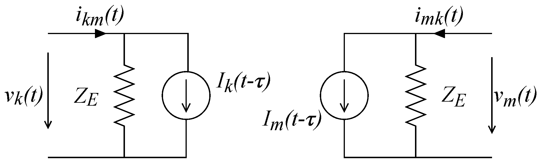
3.3. Transmission Line

The travelling wave transmission line model has two advantages over the Pi-line model. For long lines, it is more accurate than the Pi-line model and it enables the decoupling of network sections as shown in Section 3.4.

The most simple transmission line model, the Bergeron model, which is also implemented in the simulator, is based on the telegrapher’s equation. This model is derived from the equations of a lossless line and losses are only approximated in a second step. The model parameters are computed for a fixed frequency, which means that they are inaccurate for deviating frequencies. Actually, the line parameters vary, especially for high frequencies, where the skin effect has a notable impact. Dynamic phasors have an advantage in this regard, because, in the best case, each phasor represents a narrow frequency band signal. Each of these phasors can be treated differently by computing the transmission line parameters for the center frequency of these bands.

The Bergeron model applied to nodal analysis can decouple the two end nodes of a transmission line. This means two network sections that are only connected by transmission lines can be solved separately and in parallel. Instead of having one large system matrix, two smaller system matrices can be computed. These two subsystems are only coupled by their source vectors, which depend on the solution of the other subsystem from the previous time step.

This transmission line model can only be used for lines, where the delay is larger than the simulation time step. Therefore, this model is usually not suitable for simulations with large time steps or networks with very short lines.

First, the commonly used EMT domain model is described. Subsequently, this model is adapted for DP variables. The Bergeron model is derived from the wave propagation Equation (24) of a lossless line with per line length inductance $L^{\prime }$ and capacitance $C^{\prime }$ [25].

$$\begin{array}{cc}\hfill -\frac{\partial v(x,t)}{\partial x}& =L^{\prime }\frac{\partial i(x,t)}{\partial t}\hfill \end{array}$$

(23)

$$\begin{array}{cc}\hfill -\frac{\partial i(x,t)}{\partial x}& =C^{\prime }\frac{\partial v(x,t)}{\partial t}\hfill \end{array}$$

(24)

The lossless line can be represented in nodal analysis by impedances and current sources, as depicted in Figure 3, with $Z_E=Z_C$ and the values of the current sources being computed from the currents at time $t-\tau$ [23].

The time constant $\tau$ and the characteristic impedance $Z_C$ are calculated from the line length d, as follows:

$$Z_C=\sqrt{L^{\prime }/C^{\prime }}\tau =d\sqrt{L^{\prime }{C}^{\prime }}.$$

(25)

Line losses can be approximated in the model by adding a resistance at the start and end of each line section and modifying the history current sources. The equivalent impedance becomes $Z_E=Z+R/4$ and the history current is calculated as:

$$\begin{array}{cc}\hfill I_k(t-\tau )& =\frac{-Z}{{(Z+R/4)}^2}(v_m(t-\tau )+(Z-R/4)·i_{mk}(t-\tau ))\hfill \\ \hfill & -\frac{R/4}{{(Z+R/4)}^2}(v_k(t-\tau )+(Z-R/4)·i_{km}(t-\tau )),\hfill \end{array}$$

(26)

with an analogous expression for $I_m(t-\tau )$.

It is necessary to understand how the time delay in (26) affects the DP variables in order to develop the dynamic phasor model. A bandpass signal $s\left(t\right)$ can be expressed as a baseband signal $f\left(t\right)$ shifted by ${\omega }_s$ (27). The Fourier transform $S\left(\omega \right)$ is given by (28).

$$s\left(t\right)=\mathbf{Re}\left\{f\left(t\right)e^{j{\omega }_{s}t}\right\}$$

(27)

$$S\left(\omega \right)=\int f\left(t\right)e^{j{\omega }_{s}t}{e}^{-j\omega t}d\omega =F(\omega -{\omega }_s)$$

(28)

A time shift $\tau$ becomes a multiplication by $e^{-j\tau \omega }$ in the frequency domain. Hence, the time shifted signal can be computed from the Fourier transform, as follows:

$$s(t-\tau )=\mathbf{Re}\left\{\int F(\omega -{\omega }_s)e^{-j\tau \omega }{e}^{j\omega t}d\omega \right\}.$$

(29)

For $y=\omega -{\omega }_s$, (29) becomes

$$\begin{array}{cc}\hfill s(t-\tau )& =\mathbf{Re}\left\{\int F\left(y\right)e^{-j\tau (y+{\omega }_s)}{e}^{j(y+{\omega }_s)t}dy\right\}\hfill \\ \hfill & =\mathbf{Re}\left\{e^{j({\omega }_{s}t-\tau {\omega }_s)}\int F\left(y\right)e^{-j\tau y}{e}^{jyt}dy\right\}\hfill \\ \hfill & =\mathbf{Re}\left\{e^{j({\omega }_{s}t-\tau {\omega }_s)}f(t-\tau )\right\}.\hfill \end{array}$$

(30)

This means that the time shift leads to an additional phase shift $e^{-j\tau {\omega }_s}$ for the DP variables. Therefore, (26) expressed in terms of dynamic phasors results in (31).

$$\begin{array}{cc}\hfill \langle I_k(t-\tau )\rangle & =e^{-j\tau {\omega }_s}[\frac{-Z}{{(Z+R/4)}^2}(\langle v_m(t-\tau )\rangle +(Z-R/4)·\langle i_{mk}(t-\tau )\rangle )\hfill \\ \hfill & -\frac{R/4}{{(Z+R/4)}^2}(\langle v_k(t-\tau )\rangle +(Z-R/4)·\langle i_{km}(t-\tau )\rangle )]\hfill \end{array}$$

(31)

In a dynamic phasor simulation, the carrier or shifting frequency is only considered after the actual simulation in a post processing step. Without the additional phase shift, the time delay does not affect the carrier signal and the simulation results would be incorrect.

A small example that consists of a voltage source and resistance connected by a transmission line is simulated in order to demonstrate the correctness of the DP model. The parameters of the components can be found in

Table 2. Transmission line example parameters.

Attribute	Value
$V_{sec}$	100 $\mathrm{k}$$\mathrm{V}$
R	5 $\mathsf{\Omega }$
L	$0.16$$\mathrm{H}$
C	1 $\mathsf{\mu }$$\mathrm{F}$
$R_{load}$	10 $\mathrm{k}$$\mathsf{\Omega }$

.

The comparison of DP to EMT simulation shows that the results are the same if the phase shift is correctly taken into account. At the beginning, transients are visible because the simulation does not start from steady state. Figure 4 compares the current through the transmission line for the DP and EMT model.

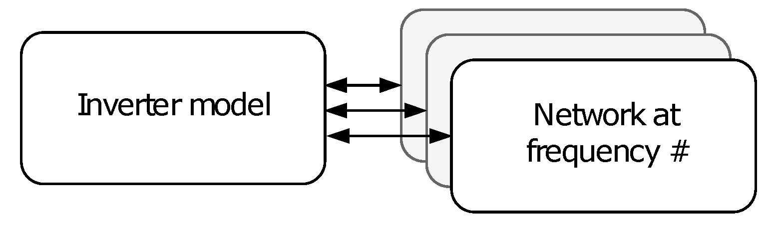
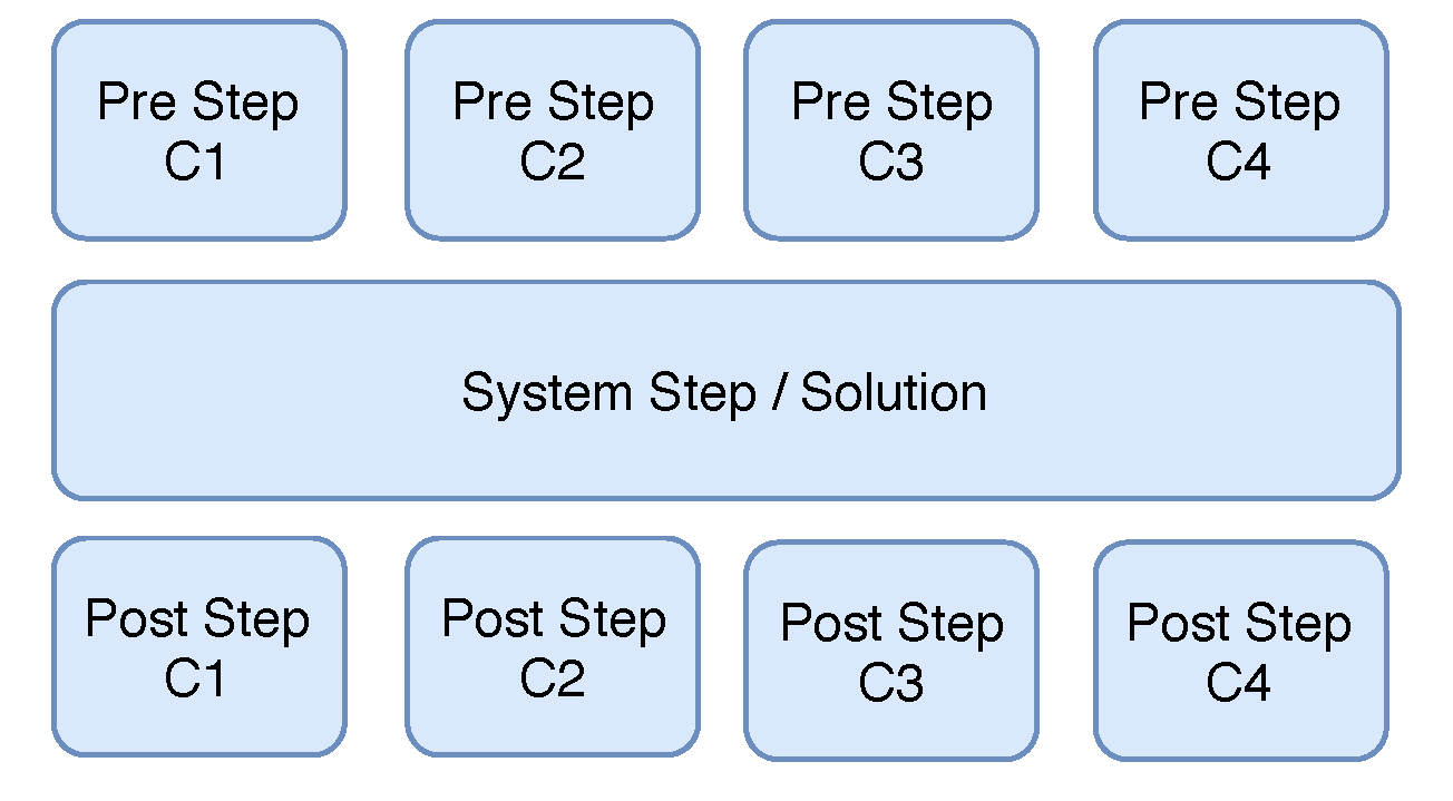
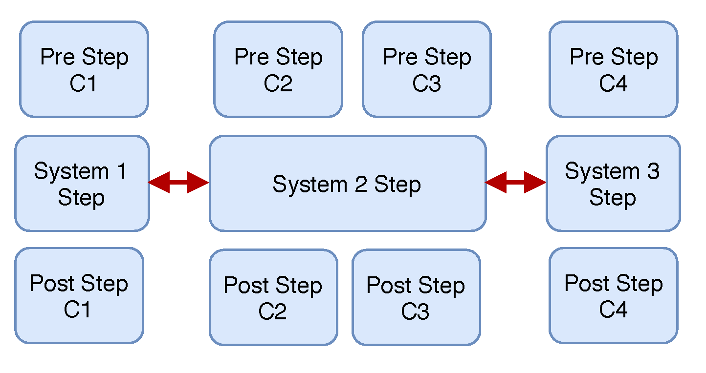
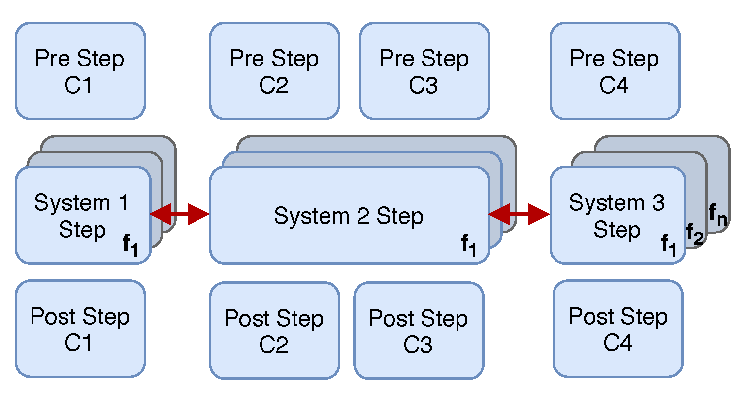
3.4. Parallelization of Subsystems and Frequency Bands

First, the solution process of the DPsim simulator is reviewed, including the decoupling and parallelization implemented before power electronics were added to the simulator. Subsequently, this concept is extended by a method that supports a more efficient computation of networks with many harmonics.

The main idea behind DPsim is to compute the network solution with nodal analysis [26] applied to DP variables. Therefore, the solution for one simulation step consists of three parts:

• calculating component states required for the network solution,
• solving the network,
• updating remaining component states from the network solution.

Most component related tasks can be executed in parallel as shown in Figure 5, because the components do not interact with each other directly, but only through the network.

However, the network simulation is often the bottleneck. The TLM is commonly used in EMT real-time simulation in order to decouple the network and compute the subsystems in parallel, as shown in Figure 6. Because DPsim is computing DP variables, the EMT transmission line model has to be adapted to the DP domain, as described in Section 3.3.

As mentioned earlier, one of the main disadvantages of the dynamic phasor approach is that the more phasors are used to represent a time domain variable, the larger becomes the number of equations and variables to solve for. This is especially a problem for the network solution, which can be already very large because of the number of network nodes. The idea is to split the network solution into separate solutions for each frequency band, as depicted in Figure 7. The underlying assumption is that the network is usually composed of linear components. An approach on how to separate nonlinearities from the network model is proposed in [27]. Nonlinearities are implemented in the components connected to the network and they can be treated separate from the network solution. Hence, the network solution does not feature cross frequency coupling.

4. Results

The first section demonstrates a scenario featuring the averaged DP inverter model integrated into DPsim in order to support the analysis of future energy systems with large shares of inverter interfaced renewable sources. The simulation scenario is a variation of the CIGRE MV network with a high share of renewable sources represented by averaged inverter models with controls, see Section 3.1. The results show that a DP simulation can be as accurate as an EMT simulation for small simulation time steps. For larger simulation steps, where the EMT simulation does not return useful results anymore, the DP results show still a good accuracy while tending towards conventional phasor results.

Section 4.2 demonstrates the extension of the inverter model by harmonics, which results in a very detailed representation of a switched inverter model. This model is compared to a switching EMT inverter model implemented in Matlab/Simulink™. The detailed dynamic phasor model, including harmonics, leads to a large set of equations, which has an impact on the computation time, especially for the network solution.

Section 4.3 presents results for the parallelization of the detailed inverter model simulation. The method is explained in Section 3.4 and it addresses the problem by splitting the solution of the network into smaller tasks, which can be executed in parallel.

4.1. Averaged Inverter Model with Controls

This section shows an analysis of the simulation results that were obtained for a scenario with a high penetration of renewables using two types of component models: DP and EMT models. That is, all types of grid components in the simulation (transformers, lines, loads, and renewable sources) are represented by DP or EMT models. The underlying research question is how an increase of the simulation step affects the accuracy of the simulation results when using these two modeling approaches. At this point, it should be noted that a fixed-step solver is applied, which is particularly suitable for real-time simulation, and the trapezoidal rule for numerical integration.

The two modeling approaches are investigated in the context of a grid simulation at medium voltage level, where a high penetration of renewables requires an adequate simulation of the emerging grid dynamics. The simulation scenario encompasses the first feeder of the CIGRE MV grid, see Figure 8, at a nominal voltage of $20\mathrm{k}\mathrm{V}$, and with a total load power of $4319\mathrm{k}\mathrm{W}$. In the following, a scenario is considered with 100% penetration of photovoltaic systems, i.e., the installed nominal power of the PV systems is equal to the total load power. For this, PV systems of equal size are connected to nodes N3 to N11 of the feeder. The PV systems are represented by inverters using an averaged switching model. The inverters operate in grid feeding mode targeting the injection of active and reactive power reference values. Section 3.1 outlines further details on the averaged inverter model and its control.

First, EMT and DP simulations are both executed with characteristic simulation steps. The simulations are conducted with a duration of $5\mathrm{s}$ and apply a load step event at time instant $2\mathrm{s}$ by increasing the load power about $1500\mathrm{k}\mathrm{W}$ at node N11. Figure 9 shows the current through the line L11-10 $100\mathrm{m}\mathrm{s}$ before and $200\mathrm{m}\mathrm{s}$ after the load step event. The DP simulation results have been analogous to the EMT results linearly interpolated to $50\mathsf{\mu }\mathrm{s}$ and additionally shifted back by $50\mathrm{Hz}$.

The DP and EMT simulation results are compared for characteristic simulation steps against a reference simulation, which was conducted as EMT simulation with a simulation step of $50\mathsf{\mu }\mathrm{s}$. Figure 9a demonstrates that, for a step size of $100\mathsf{\mu }\mathrm{s}$, the simulation results in the DP and EMT domain still match well with the results of the reference simulation. When increasing the simulation step to 1 ms, see Figure 9b, the results still appear very similar. However, it is noteworthy that both DP and EMT results deviate from the reference during the first oscillatory cycle. This seems to be feasible as a simulation with a step size of $1\mathrm{m}\mathrm{s}$ is not able to capture the wide frequency spectrum occurring after the load step, for both the EMT and the $50\mathrm{Hz}$ shifted DP signal. Yet, except from this deviation during the first oscillatory cycle, the signals match well in the following oscillatory cycles after the load step event.

For larger simulation steps of $5\mathrm{m}\mathrm{s}$ and $10\mathrm{m}\mathrm{s}$, see Figure 9c,d, the EMT results differ significantly from the reference results. Instead, the DP results remain quite accurate for these larger simulation steps. In particular, it is remarkable that the DP results still show the evolution of the oscillations towards the steady state behaviour well.

In the following, the difference of DP and EMT simulation results is quantatively investigated with respect to the reference results. For this, the DP and EMT simulation results obtained with steps in the range from $100\mathsf{\mu }\mathrm{s}$ to $20\mathrm{m}\mathrm{s}$ are considered. The step size is increased by $200\mathsf{\mu }\mathrm{s}$ in the microseconds range and by $1\mathrm{m}\mathrm{s}$ in the milliseconds range. For DP and EMT results of the line current L11-10, the root mean squared error (RMSE) is calculated with respect to the reference results. The evolution of the RMSE that is depicted in Figure 10 confirms that both DP and EMT results are quite accurate for simulation steps up to $1\mathrm{m}\mathrm{s}$.

In the range from $2\mathrm{m}\mathrm{s}$ to $20\mathrm{m}\mathrm{s}$, the RMSE of the EMT results increases tremendously. This seems reasonable as in EMTP-based simulation it is well known that an appropriate accuracy is obtained only for simulation steps below $10\%$ of the minimum cycle duration that is to be simulated [28]. This requires a simulation step below $2\mathrm{m}\mathrm{s}$ for $50\mathrm{Hz}$ signals. As the simulated signals are shifted by $50\mathrm{Hz}$ in the DP domain, the RMSE of the DP results remains very low with respect to the EMT error.

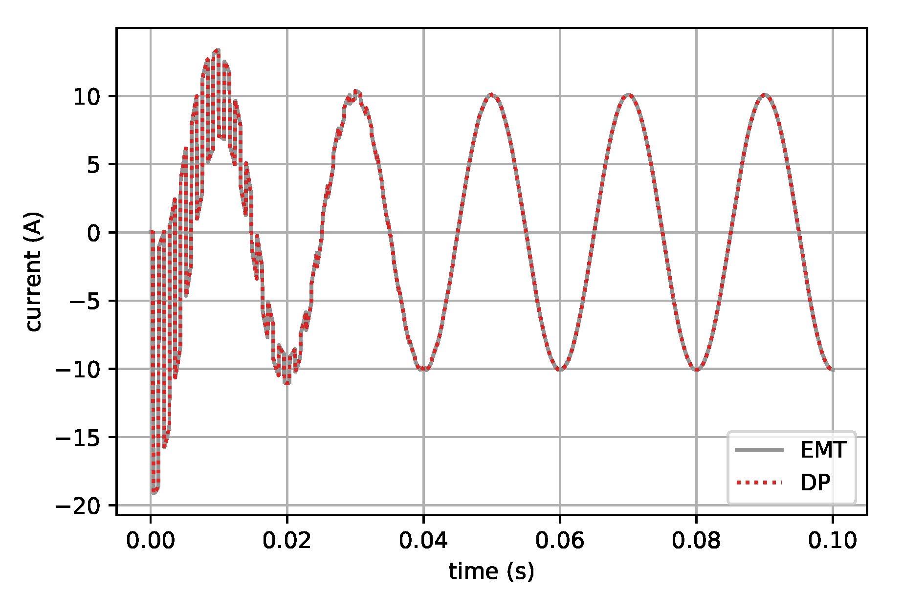
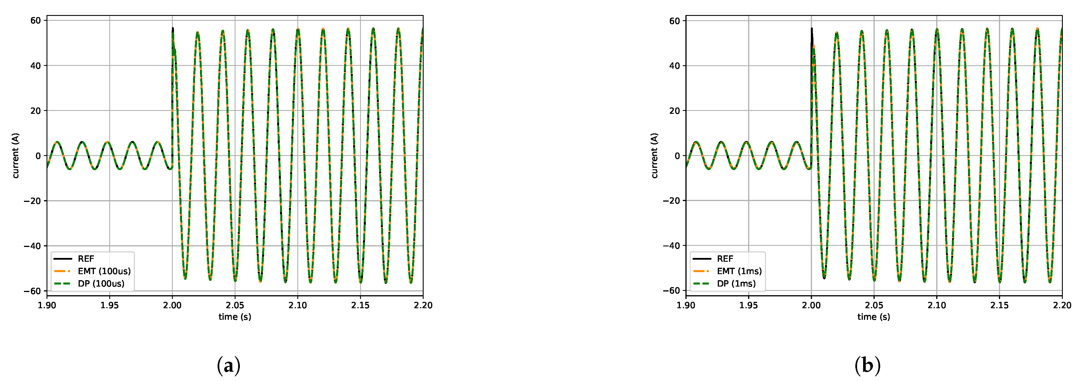
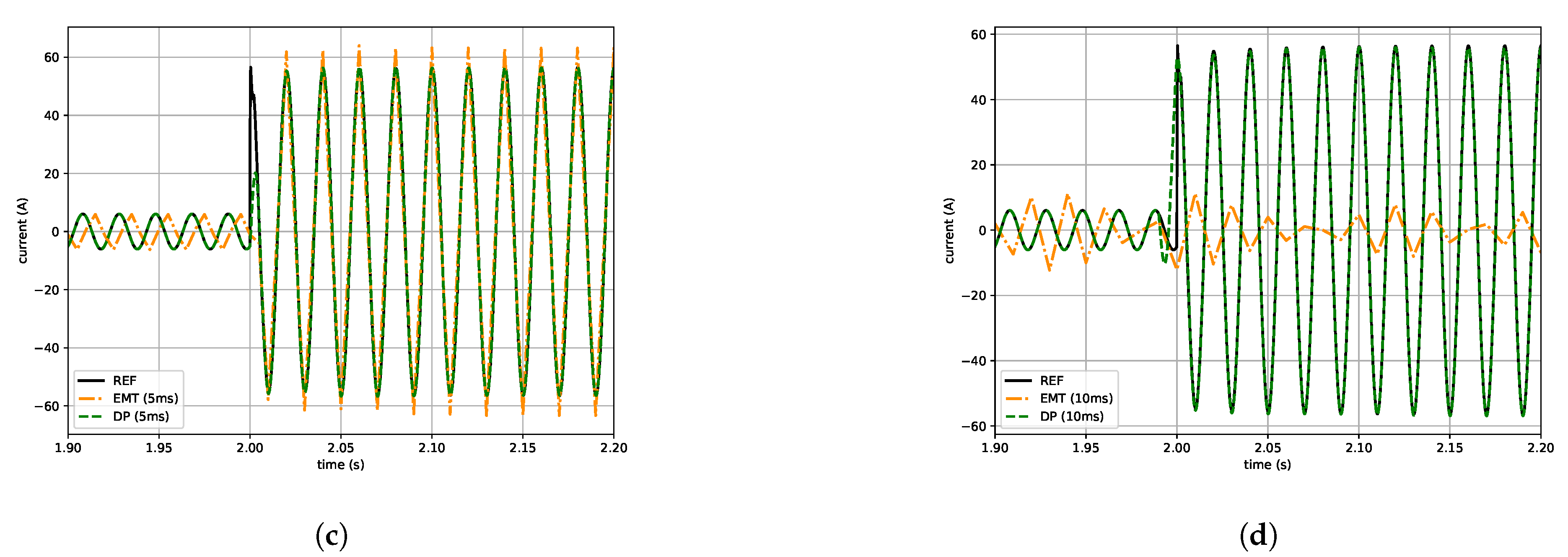
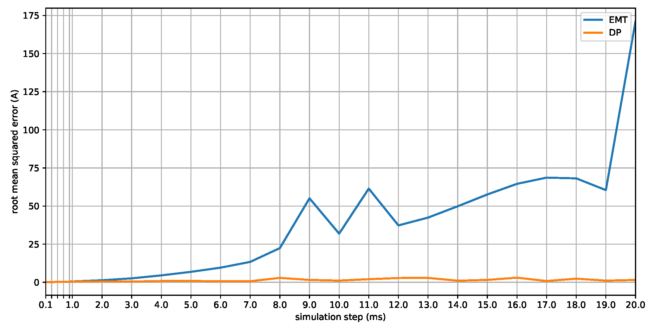
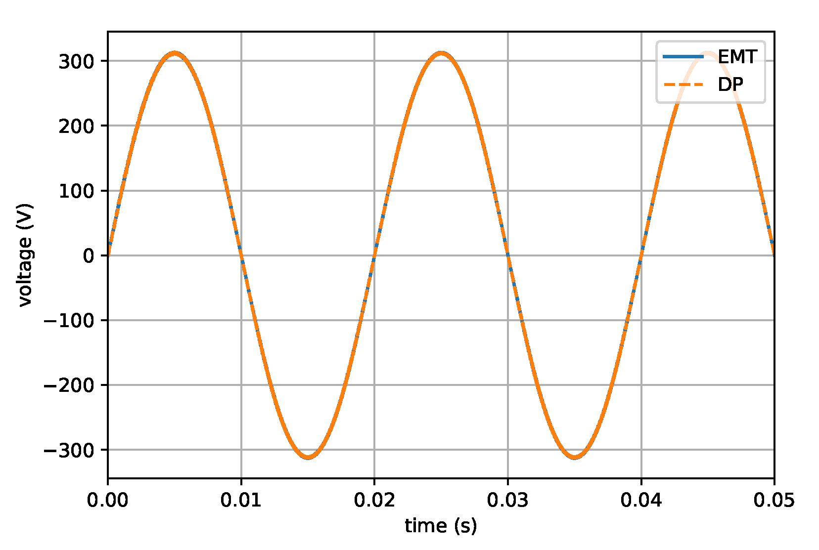
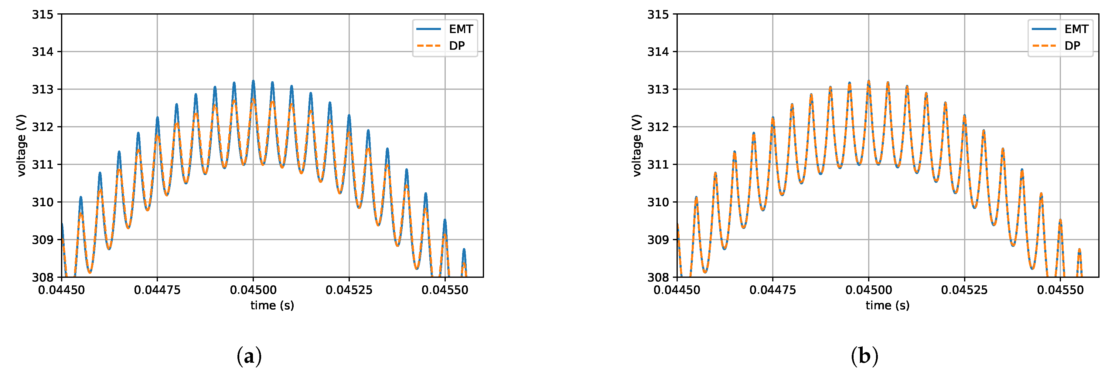
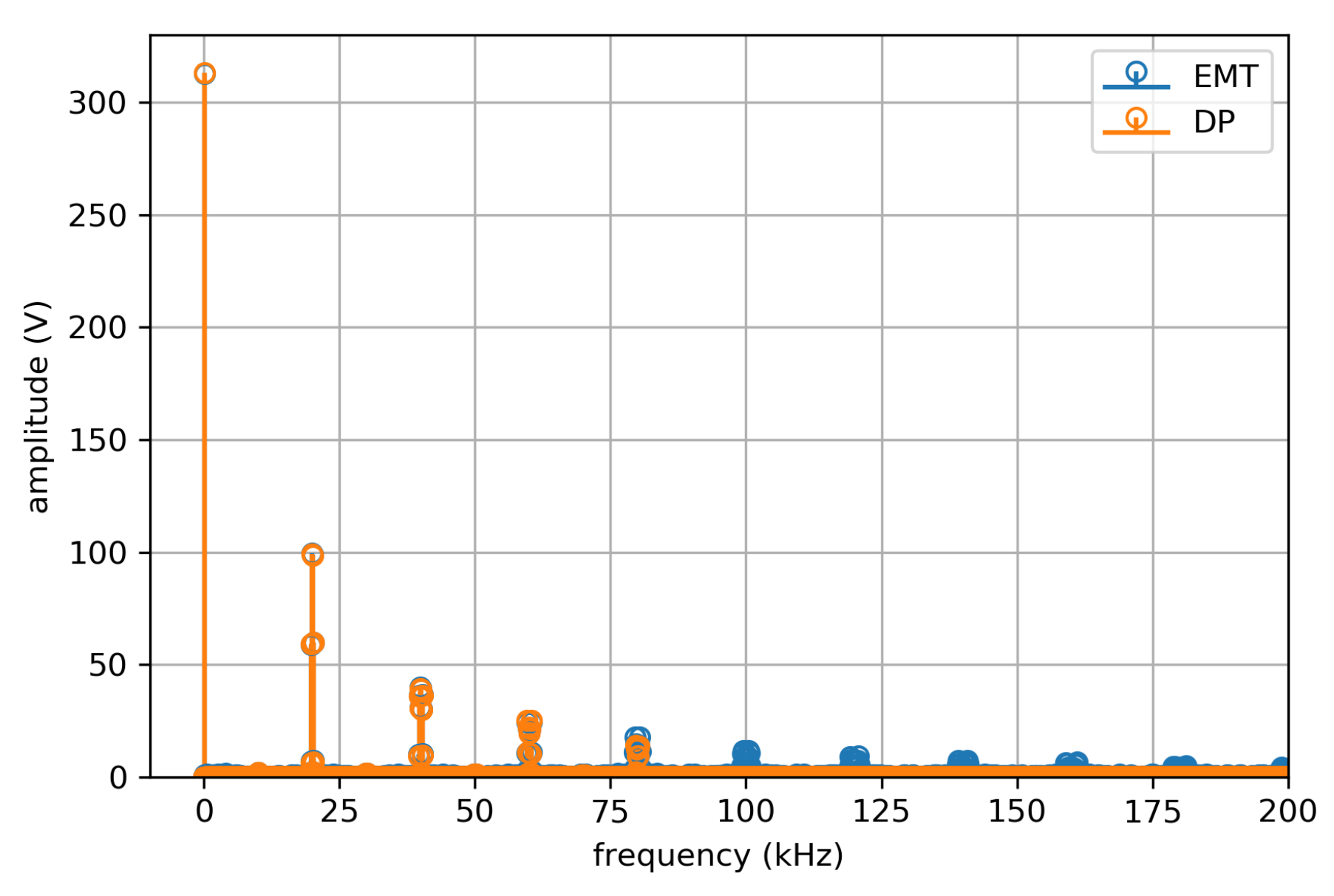
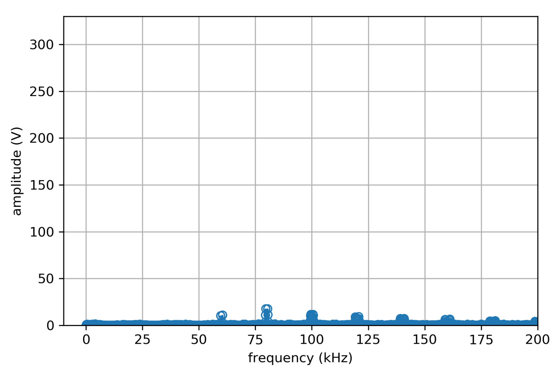
4.2. Inverter Model Including Harmonics

One advantage of dynamic phasors is the ability to include selected harmonics, which is particularly interesting for power electronics modelling. The simulations presented in this section feature a DP inverter model that extends the inverter used in Section 4.1 by harmonics that are based on harmonic analysis as explained in Section 3.2. This model, which does not include switches, is validated against a switching Matlab/Simulink™ EMT model. For this comparison, the regular sampling Equation (20) are used in the harmonic analysis.

The inverter model is connected to an equivalent grid model composed of an impedance and a voltage source. Figure 11 depicts the circuit and

Table 3. Inverter simulation example parameters.

Attribute	Value
$R_1$	$0.1$$\mathsf{\Omega }$
$L_1$	600 $\mathsf{\mu }$$\mathrm{H}$
$R_2$	$0.1$$\mathsf{\Omega }$
$L_2$	150 $\mathsf{\mu }$$\mathrm{H}$
$R_g$	$0.001$$\mathsf{\Omega }$
$L_g$	$0.001$$\mathrm{H}$
C	10 $\mathsf{\mu }$$\mathrm{F}$
$R_C$	1 $\mathsf{\mu }$$\mathsf{\Omega }$

lists the parameters.

The DP inverter model can be simulated with a varying number of harmonics. Here, eight and 28 additional harmonics are considered. Figure 12 shows the voltage at the output filter capacitor of the circuit depicted in Figure 11 for DP with eight additional harmonics and the Simulink EMT model. Figure 13a,b depict a smaller time interval of the simulation and demonstrate the difference in accuracy when considering different numbers of harmonics and dynamic phasors, respectively. The mean absolute error (MAE) for the results with eight harmonics is about $0.2$$\mathrm{V}$, whereas the MAE for 28 harmonics is 20% smaller.

The results of the simulation with eight harmonics do not represent the ripple as accurately. It can determined from harmonic analysis that in this scenario, eight harmonics account for the phasors that are larger than 10% of the fundamental, whereas 28 harmonics covers all harmonics larger than 1% of the fundamental. In this example, the grid harmonics are considered up to the index $n_{max}=7$, whereas the maximum switching harmonic is $m_{max}=8$.

Figure 14 depicts the spectrum computed from the DP and EMT signal and shows how frequencies higher than the fundamental are accurately represented in the DP results up to a certain point, which depends on the number of dynamic phasors. Figure 15 presents the difference between the two spectra. It can be seen that high sideband harmonics are missing as well as high harmonics of the switching frequency, whereas lower harmonics are covered by the DP model.

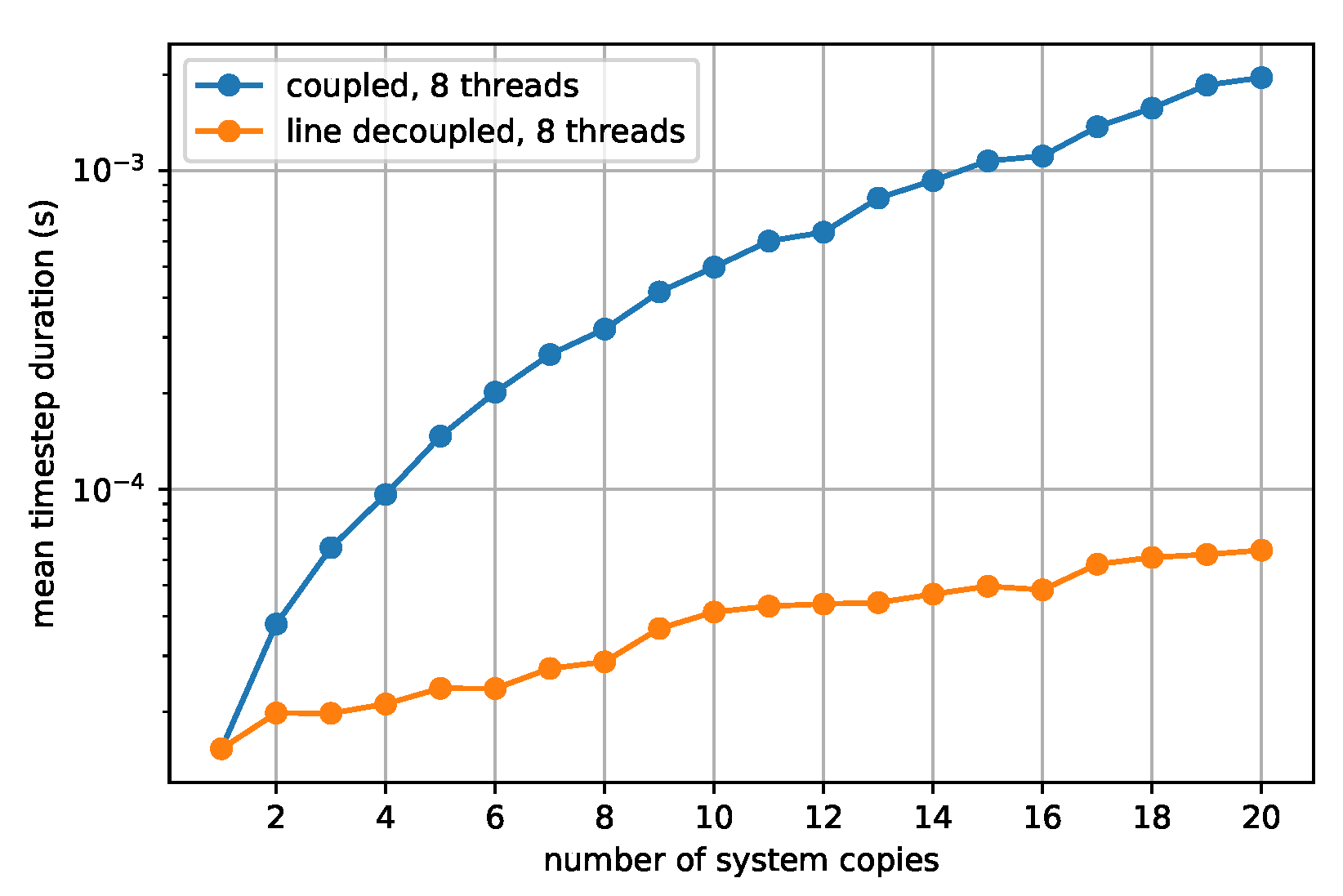
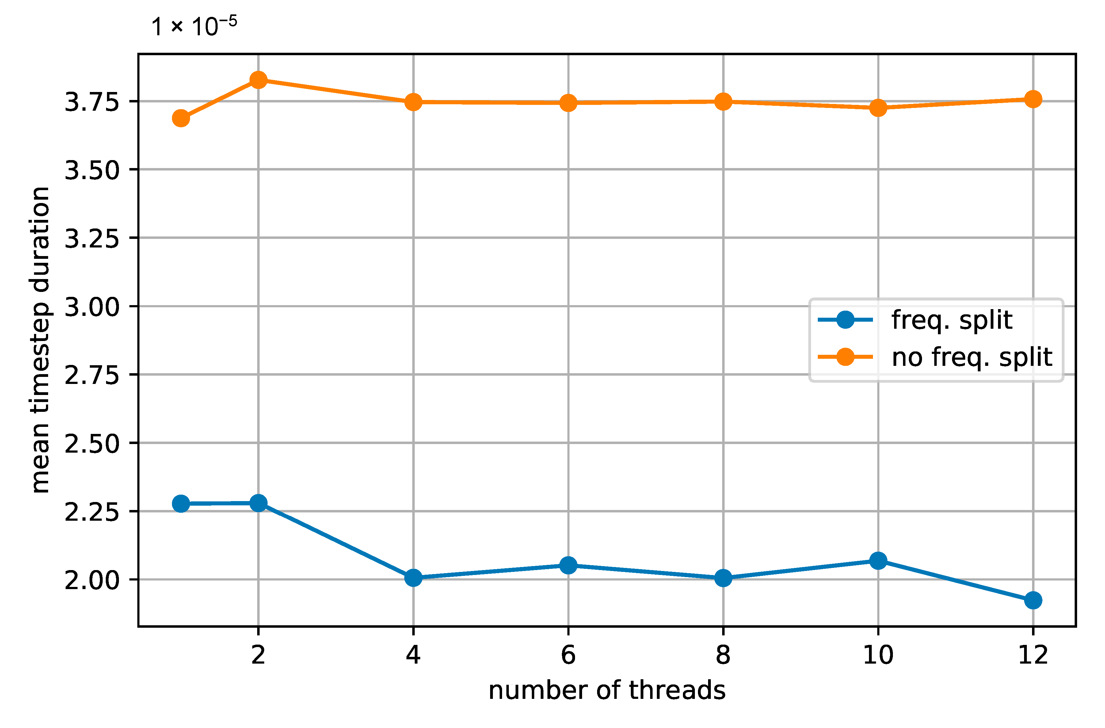
4.3. Parallelization for Large Systems and Power Electronics

The previous two sections only considered the modelling accuracy, but not the simulation performance in terms of computation time, which is important for real-time execution. Especially, the DP inverter model including harmonics, described in Section 3.2, increases the number of variables drastically with considerable impact on the computation time. To improve computation time, DPsim parallelizes tasks that are not depending on each other. Larger tasks, such as the network solution, require decoupling to be able to split the task into smaller tasks that can be executed in parallel, as explained in Section 3.4.

The results for TLM decoupling in DP simulations were already presented in [15], but for consistency with the following parallelization results, the study has been repeated on different hardware, having two Intel Xeon E5-2643 v4 CPUs clocked at 3.4 GHz with 12 cores in total, running Fedora 30, and using the most recent version of DPsim. From Figure 16, it can be seen that the simulation using TLM decoupling outperforms the coupled simulation by up to about three times for 20 copies. The number of copies refers to the number of WSCC nine-bus instances that are interconnected through transmission lines for the TLM case or Pi-lines for the coupled case, respectively. All of the simulations are using eight threads in this scenario. Although it is clear that the transmission line model decoupling is better in terms of computation time, it should be noted that the transmission line model is not equivalent to the Pi-line model and it yields different simulation results.

The inverter model simulated in Section 4.2 and described in Section 3.2 results in many phasors of different shifting frequencies being fed into the network. At first glance, this seems to be a disadvantage of dynamic phasors, because the simulation accuracy is increased at the cost of increasing the number of equations with every phasor. As explained in Section 4.2, even considering only harmonics of at least 10% of the fundamental requires eight additional phasors. Hence, if no measures are taken, the network equation set does not only grow quadratically with the number of network nodes, but also the number of considered harmonics. To overcome this limitation of dynamic phasors, the spectral parallelization that is explained in Section 3.4 is applied to the grid connected inverter example presented in Section 4.2.

It can be seen in Figure 17 that this network split with regard to frequencies already improves the computation time significantly, even for the small example circuit that is depicted in Figure 11. The computation time is almost two times shorter if the network is solved separately for each frequency band. Besides, Figure 17 demonstrates the performance for different numbers of threads. As expected, the improvement is not noticeable when the system is not split frequency-wise. If the system is split, a higher number of threads seems to be beneficial, but the impact is not very large because the considered system is small when compared to the simulation of a complete grid.

The inverter model is still computed sequentially, as depicted in Figure 2 but the network solution is computed separately for each set of dynamic phasor variables that are associated to one shifting frequency. In the open loop case, the computation of harmonics inside the inverter model could be parallelized as well, but, in the general case, there could be cross frequency coupling, for example, by means of the inverter control.

5. Conclusions

The presented simulation results fall into two groups: power electronics modelling and real-time capability advancements by parallelization. The power electronics related results demonstrate that dynamic phasors can bridge the gap between the simulation of EMT and conventional phasor models and provide an easy method to represent either of the two modelling domains, depending on the selected simulation step. When compared to EMT models of switching power electronics, dynamic phasors allow for the user to determine and only simulate the harmonics that are relevant. However, this also requires the user to find out the relevant harmonics in advance before running the simulation. A tool to provide this information to the user automatically would be beneficial in the future. The averaged model could be used in transient stability analysis and for testing frequency control techniques. Extending the set of controllers by grid forming controllers would enable the analysis of high frequency variation conditions. The detailed inverter model featuring harmonics allows for the user to investigate the interaction of inverter dynamics at high frequencies.

The second group of results, related to advancements by parallelization, is crucial to understand what methods can be effectively used to reduce the computation time and ensure real-time execution for small time steps in the range of milli and micro seconds for real large-sized grids. Large-sized grids may be simulated in real-time to conduct controller-in-the-loop (CiL) experiments and investigate wide area oscillations. Smaller grids can be simulated at smaller time steps for hardware-in-the-loop (HiL) experiments. As demonstrated in Section 3.4, these methods can be derived from techniques employed in EMT real-time simulation or new methods specifically introduced for dynamic phasors. While the dynamic phasor based transmission line method adopts a well known method applied in EMT real-time simulation, the parallelization of network frequencies mitigates the disadvantage of dynamic phasors. A combination of subsystem and frequency wise parallelization improves the real-time capability of DPsim for large grids featuring detailed power electronics models, which is necessary for the simulation of future power systems.

References

1. Faruque, M.O.; Strasser, T.; Lauss, G.; Jalili-Marandi, V.; Forsyth, P.; Dufour, C.; Dinavahi, V.; Monti, A.; Kotsampopoulos, P.; Martinez, J.A.; et al. Real-time simulation technologies for power systems design, testing, and analysis. IEEE Power Energy Technol. Syst. J. 2015, 2, 63–73. [Google Scholar] [CrossRef]
2. Chen, Y.; Dinavahi, V. FPGA-based real-time EMTP. IEEE Trans. Power Deliv. 2008, 24, 892–902. [Google Scholar] [CrossRef]
3. Razzaghi, R.; Paolone, M.; Rachidi, F. A general purpose FPGA-based real-time simulator for power systems applications. In Proceedings of the IEEE PES ISGT Europe 2013, Lyngby, Denmark, 6–9 October 2013; pp. 1–5. [Google Scholar]
4. Milton, M.; Benigni, A.; Bakos, J. System-level, FPGA-based, real-time simulation of ship power systems. IEEE Trans. Energy Convers. 2017, 32, 737–747. [Google Scholar] [CrossRef]
5. Li, Q.; Xiang, Y.; Mu, Q.; Zhang, X.; Li, X.; He, G. Exploration of FPGA-based electromagnetic transient real-time simulation system design using high-level synthesis. J. Eng. 2018, 2019, 1217–1220. [Google Scholar] [CrossRef]
6. Hernandez, M.E.; Ramos, G.A.; Lwin, M.; Siratarnsophon, P.; Santoso, S. Embedded real-time simulation platform for power distribution systems. IEEE Access 2017, 6, 6243–6256. [Google Scholar] [CrossRef]
7. Marti, J.R.; Dommel, H.W.; Bonatto, B.D.; Barrete, A.F. Shifted Frequency Analysis (SFA) concepts for EMTP modelling and simulation of Power System Dynamics. In Proceedings of the Power Systems Computation Conference (PSCC), Wroclaw, Poland, 18–22 August 2014; pp. 1–8. [Google Scholar]
8. Strunz, K.; Shintaku, R.; Gao, F. Frequency-adaptive network modeling for integrative simulation of natural and envelope waveforms in power systems and circuits. IEEE Trans. Circuits Syst. Regul. Pap. 2006, 53, 2788–2803. [Google Scholar] [CrossRef]
9. Demiray, T.; Andersson, G.; Busarello, L. Evaluation study for the simulation of power system transients using dynamic phasor models. In Proceedings of the 2008 IEEE/PES Transmission and Distribution Conference and Exposition: Latin America, Bogota, Colombia, 13–15 August 2008; pp. 1–6. [Google Scholar]
10. Marti, A.T.J.; Jatskevich, J. Transient Stability Analysis Using Shifted Frequency Analysis (SFA). In Proceedings of the 2018 Power Systems Computation Conference (PSCC), Dublin, Ireland, 11–15 June 2018; pp. 1–7. [Google Scholar]
11. Sanders, S.R.; Noworolski, J.M.; Liu, X.Z.; Verghese, G.C. Generalized averaging method for power conversion circuits. IEEE Trans. Power Electron. 1991, 6, 251–259. [Google Scholar] [CrossRef] [Green Version]
12. Holmes, D.G.; Lipo, T.A. Pulse Width Modulation for Power Converters: Principles and Practice; John Wiley & Sons: Hoboken, NJ, USA, 2003; Volume 18. [Google Scholar]
13. Stevic, M.; Estebsari, A.; Vogel, S.; Pons, E.; Bompard, E.; Masera, M.; Monti, A. Multi-site European framework for real-time co-simulation of power systems. IET Gener. Transm. Distrib. 2017, 11, 4126–4135. [Google Scholar] [CrossRef] [Green Version]
14. Monti, A.; Stevic, M.; Vogel, S.; De Doncker, R.W.; Bompard, E.; Estebsari, A.; Profumo, F.; Hovsapian, R.; Mohanpurkar, M.; Flicker, J.D.; et al. A Global Real-Time Superlab: Enabling High Penetration of Power Electronics in the Electric Grid. IEEE Power Electron. Mag. 2018, 5, 35–44. [Google Scholar] [CrossRef] [Green Version]
15. Mirz, M.; Vogel, S.; Reinke, G.; Monti, A. DPsim—A dynamic phasor real-time simulator for power systems. SoftwareX 2019, 10, 100253. [Google Scholar] [CrossRef]
16. Vogel, S.; Mirz, M.; Razik, L.; Monti, A. An open solution for next-generation real-time power system simulation. In Proceedings of the 2017 IEEE Conference on Energy Internet and Energy System Integration (EI2), Beijing, China, 26–28 November 2017; pp. 1–6. [Google Scholar]
17. Razik, L.; Mirz, M.; Knibbe, D.; Lankes, S.; Monti, A. Automated deserializer generation from CIM ontologies: CIM++—An easy-to-use and automated adaptable open-source library for object deserialization in C++ from documents based on user-specified UML models following the Common Information Model (CIM) standards for the energy sector. Comput. Sci. Res. Dev. 2018, 33, 93–103. [Google Scholar]
18. Maas, S.A. Nonlinear Microwave and RF Circuits; Artech House: London, UK, 2003. [Google Scholar]
19. Proakis, J.G.; Salehi, M.; Zhou, N.; Li, X. Communication Systems Engineering; Prentice Hall New Jersey: Upper Saddle River, NJ, USA, 1994; Volume 2. [Google Scholar]
20. Henschel, S. Analysis of Electromagnetic and Electromechanical Power System Transients with Dynamic Phasors. Ph.D. Thesis, University of British Columbia, Vancouver, BC, Canada, 1999. [Google Scholar]
21. Zhang, P.; Marti, J.R.; Dommel, H.W. Shifted-frequency analysis for EMTP simulation of power-system dynamics. IEEE Trans. Circuits Syst. I Regul. Pap. 2010, 57, 2564–2574. [Google Scholar] [CrossRef]
22. Demiray, T. Simulation of Power System Dynamics Using Dynamic Phasor Models. Ph.D. Thesis, ETH Zurich, Zurich, Switzerland, 2008. [Google Scholar]
23. Dommel, H.W. Digital Computer Solution of Electromagnetic Transients in Single-and Multiphase Networks. IEEE Trans. Power Appar. Syst. 1969, PAS-88, 388–399. [Google Scholar] [CrossRef]
24. Rocabert, J.; Luna, A.; Blaabjerg, F.; Rodríguez, P. Control of Power Converters in AC Microgrids. IEEE Trans. Power Electron. 2012, 27, 4734–4749. [Google Scholar] [CrossRef]
25. Watson, N.; Arrillaga, J.; Arrillaga, J. Power Systems Electromagnetic Transients Simulation; IET: Stevenage, UK, 2003; Volume 39. [Google Scholar]
26. Ruehli, A.; Brennan, P. The modified nodal approach to network analysis. IEEE Trans. Circuits Syst. 1975, 22, 504–509. [Google Scholar]
27. Benigni, A.; Monti, A. A parallel approach to real-time simulation of power electronics systems. IEEE Trans. Power Electron. 2014, 30, 5192–5206. [Google Scholar] [CrossRef]
28. de Siqueira, J.C.G.; Bonatto, B.D.; Martí, J.R.; Hollman, J.A.; Dommel, H.W. Optimum time step size and maximum simulation time in EMTP-based programs. In Proceedings of the 2014 Power Systems Computation Conference, Wroclaw, Poland, 18–22 August 2014; pp. 1–7. [Google Scholar]
Figure 1. Averaged inverter model with controls.
Energies 13 03879 g001
Figure 2. Separate computation of nonlinear inverter model from the network that is split by shifting frequency.
Energies 13 03879 g002
Figure 3. Equivalent circuit for a lossless line.
Energies 13 03879 g003
Figure 4. Comparison of DP and electromagnetic-transient (EMT) resistor current results for the transmission line model.
Energies 13 03879 g004
Figure 5. Parallelization of the component step calculations.
Energies 13 03879 g005
Figure 6. Parallel solution of decoupled subsystems.
Energies 13 03879 g006
Figure 7. Parallel solution of decoupled subsystems for each set of dynamic phasors associated to the same shifting frequency.
Energies 13 03879 g007
Figure 8. Simulation scenario considering the first feeder of CIGRE MV grid.
Energies 13 03879 g008
Figure 9. Comparison of EMT and dynamic phasor (DP) simulation results with the averaged inverter model for time steps of 100   μ s (a), 1   m s (b), 5   m s (c) and 10   m s (d).
Energies 13 03879 g009aEnergies 13 03879 g009b
Figure 10. RMSE of EMT and DP simulation results with respect to the reference results.
Energies 13 03879 g010
Figure 11. Single phase inverter with LCL output filter connected to an equivalent grid represented by a voltage source with series impedance R g and L g .
Energies 13 03879 g011
Figure 12. Capacitor voltage of a DP inverter model including the fundamental and eight harmonics compared to a Simulink EMT model.
Energies 13 03879 g012
Figure 13. Ripple of the capacitor voltage of a DP inverter model including the fundamental and 8 harmonics (a) or 28 harmonics (b) as compared to a Simulink EMT model.
Energies 13 03879 g013
Figure 14. Spectrum of the DP inverter simulation with 28 harmonics as compared to Simulink EMT.
Energies 13 03879 g014
Figure 15. Difference of the spectrum of the inverter simulation with 28 harmonics compared to Simulink EMT.
Energies 13 03879 g015
Figure 16. Parallelization results for eight threads comparing different decoupling methods.
Energies 13 03879 g016
Figure 17. Parallelization results for single phase inverter.
Energies 13 03879 g017