Improving Thermochemical Energy Storage Dynamics Forecast with Physics-Inspired Neural Network Architecture

Abstract

Thermochemical Energy Storage (TCES), specifically the calcium oxide (CaO)/calcium hydroxide (Ca(OH)₂) system is a promising energy storage technology with relatively high energy density and low cost. However, the existing models available to predict the system’s internal states are computationally expensive. An accurate and real-time capable model is therefore still required to improve its operational control. In this work, we implement a Physics-Informed Neural Network (PINN) to predict the dynamics of the TCES internal state. Our proposed framework addresses three physical aspects to build the PINN: (1) we choose a Nonlinear Autoregressive Network with Exogeneous Inputs (NARX) with deeper recurrence to address the nonlinear latency; (2) we train the network in closed-loop to capture the long-term dynamics; and (3) we incorporate physical regularisation during its training, calculated based on discretized mole and energy balance equations. To train the network, we perform numerical simulations on an ensemble of system parameters to obtain synthetic data. Even though the suggested approach provides results with the error of $3.96$×${10}^{-4}$ which is in the same range as the result without physical regularisation, it is superior compared to conventional Artificial Neural Network (ANN) strategies because it ensures physical plausibility of the predictions, even in a highly dynamic and nonlinear problem. Consequently, the suggested PINN can be further developed for more complicated analysis of the TCES system.

1. Introduction

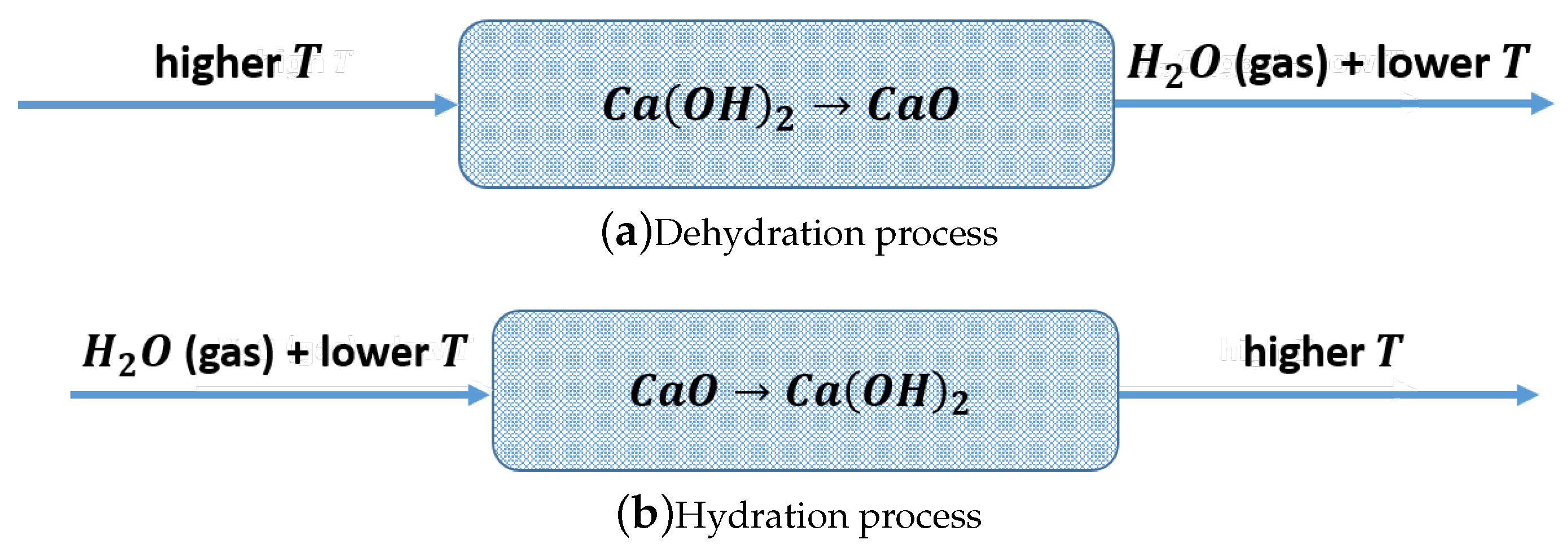
1.1. Thermochemical Energy Storage

Energy storage systems have become increasingly important in the shift towards renewable energy because of the fluctuation inherent to renewable energy generation [1,2]. Thermochemical Energy Storage (TCES) stores and releases energy in the form of heat as chemical potential of a storage material through a reversible endothermic/exothermic chemical reaction. TCES is favourable compared to sensible and latent heat storage [3,4,5] because it features a high energy density, low heat losses and the possibility to discharge the system at a relatively high and constant output temperature [6].

Numerous studies have been conducted on thermochemical energy storage in different materials, including calcium oxide [3,6], manganese oxide [7,8], barium oxide [9], zinc oxide [10], cobalt oxide/iron oxide [11], strontium bromide [12], calcium carbonate [13] and many more. In general, the chemical processes occurring on the storage material can be classified into: redox of metal oxides, carbonation/decarbonation of carbonates and hydration/dehydration of hydroxides [14]. The choice of materials depends on many criteria, one of which is the application of the energy storage. For example, in integration with Concentrated Solar Power (CSP) plants, manganese oxide is not suitable because of its high reaction temperature [6,15]. Another important aspect to consider is the practicability of the process; for example, in a calcium carbonate system, CO₂ as the side effect of the reaction has to be liquefied and results in a high parasitic loss [6,14]. Additionally, there are many more criteria to consider, such as cyclability, reaction kinetics, energy density and, most importantly, safety issues. For comprehensive reviews of varying storage materials, we refer to [14,15,16].

Recently, experimental investigations have been conducted specifically for the calcium oxide (CaO)/calcium hydroxide (Ca(OH)₂) system. One experiment investigated the material parameters (such as heat capacity and density) and the reaction kinetics [17], another experiment focused on studying the operating range, efficiency and the cycling stability of the system [18], and there was also an experiment on the feasibility of integration with concentrated solar power plants [19]. All these experiments show that CaO/Ca(OH)₂ is a very promising candidate as TCES storage material. Furthermore, it is more attractive compared to other storage materials because it is nontoxic, relatively cheap and widely available [20,21]. The system stores the heat (is charged) during the dehydration of Ca(OH)₂ by injecting dry air with higher temperature. Charging results in an endothermic reaction along with the formation of H₂O vapour and lower temperature at the outlet. It releases the heat (is discharged) during the hydration of CaO. This is achieved by injecting air with higher humidity (H₂O content) and relatively lower temperature, resulting in an exothermic reaction (see Figure 1). Note that in this case, the hydration process occurs at lower temperature relative to the dehydration process, but both processes occur at high operating temperature [22]. The reversible reaction is written as:

$$Ca{\left(OH\right)}_2+\Delta H\rightleftharpoons CaO+H_{2}O.$$

(1)

A robust operational control of this system needs an accurate and real-time capable model to predict its state of charge and health. Similar models are operationally used, namely for batteries in mobile devices [23,24]. Accordingly, numerical TCES modelling studies were conducted to predict the system’s behaviour [6,18,20,21,25]. However, the PDEs that describe the system are dynamic, highly nonlinear and strongly coupled, making the numerical simulation computationally expensive. This poses a significant hindrance on a more thorough and complex analysis of the TCES system. Estimation of the system’s state of health, for example, requires a 2D or 3D model to study the effect of the structural change due to agglomeration [26]. With increasing spatial dimension, the computational time also increases strongly. Consequently, the system is not ready yet for commercial and industrial use until a faster and accurate model is developed. In this work, we consider using Artificial Neural Network (ANN) as a cheaper alternative to the expensive existing models.

1.2. Physics-Inspired Artificial Neural Networks

Artificial Neural Networks (ANNs) have been studied and applied intensively in the past few decades. They have become very popular alongside linear regression and other techniques such as Gaussian Process Regression (GPR) and Support Vector Machine (SVM) [27]. ANNs have advantages in terms of their flexibility and better applicability to model nonlinear problems compared to linear regression and GPR [28]. Additionally, it has better scalability to larger data compared to SVM [29]. However, a detailed performance comparison of ANN with other machine learning techniques is out of the scope of this paper.

ANNs have a wide range of applications, such as image and pattern recognition, language processing, regression problems and data-driven modelling [30]. In this paper, we focus on data-driven modelling, where an ANN is trained to predict the physical behaviour of a TCES system based on available data. ANNs have been used for data-driven modelling in different fields. In hydrology [31], ANNs have been successfully applied, for example to predict rainfall-runoff [32,33], groundwater levels [34] and groundwater contamination [35]. Moreover, ANNs have been used in energy system applications [36], for example to predict the performance of [37], reliability of [38] and design [39] renewable energy systems. All these examples show that ANNs have a potential to be a quick decision making tool which is useful for many engineering and management purposes.

In previous applications of ANNs in data-driven modelling, the ANN was treated as a black box [40,41] that learns only the mathematical relationship between the input and output. In such a process, the physical relationships and scientific findings that were previously used to build governing equations of the modelled systems are completely neglected. This issue is very troublesome and needs to be addressed because real data are noisy with measurement errors, and fitting the ANN to the noisy data without any physical constraint might lead to overfitting problems [30]. Additionally, in many cases, observation data is difficult and expensive to obtain, providing users with only a limited amount of data to train the ANN. Without any physical knowledge, ANNs perform poorly when trained with a low amount of data [42,43]. Furthermore, ANNs have a very poor interpretability [44,45], meaning that there might be different combinations of ANN elements (width, depth, activation functions and parameters) that fit the training data with similar likelihood, but not all of them are physically meaningful and robust. As a result, ANN predictions might be misleading.

Implementing physical knowledge to build the ANN structure and regularisation is a potential solution to solve this issue. By combining a black box model with a white box (fully physical) model, we obtain a grey box model. In such an approach, physical theories are used in combination with observed data to improve the model prediction and plausibility [46]. Moreover, the data will help to include complex physical processes that may not be captured in currently existing white box models. There are at least two motivations to do so: to obtain a reliable surrogate model for the physics-based model for the sake of speed in real-time environments and to address situations where the underlying physics of the system are incompletely understood, so that ANNs can build on, and later exceed, the current state of physical understanding.

Several works have been conducted to develop the so-called Physics Inspired Neural Networks (PINN). In general, PINNs can be grouped into two distinguishable motivations as mentioned above. The first one applies ANNs to infer the parameter values in the governing Ordinary Differential Equations (ODEs) or Partial Differential Equations (PDEs) as well as the constitutive relationships and the differential operators [43,47], assuming that the ODEs or PDEs perfectly describe the modelled system. The second one treats the system as a complex unit that is not sufficiently represented only with simplified equations. It trains the ANN based on observation data while constraining the ANN using physically-based regularisation [42,48,49]. We aim mostly at the second motivation and ask ourselves how much of the useful knowledge contained in the PDEs can be used to inform ANNs before proceeding to train them on observation data.

Despite the success of PINN implementations in this direction, there are still some open issues that need to be addressed: (I) There is no well-defined alignment between the structure of the governing equations with the structure of the ANN. For example, most, if not all of the applications are for dynamic systems. Nevertheless, the structures of the ANNs applied do not resemble the dynamic behaviours of the systems and do not consider recurrency. (II) The focus in PINN development is more on getting high accuracy with limited amount of training data rather than improving the physical plausibility of the predictions. (III) The implementations of PINNs in previous works are mainly for relatively simple problems, and implementation to more complex problems (featuring multiple nonlinear coupled equations) has not been evident yet. In our current study, we address these three open issues.

1.3. Approach and Contributions

For dynamic and complex systems with coupled nonlinear processes such as the TCES system, we need an advanced approach to solve it using ANNs. Our approach implements physical knowledge of the system into building the ANN such as: (I) we use a Nonlinear Autoregressive Network with Exogeneous Inputs (NARX) structure. This is a form of Recurrent Neural Network (RNN), and we use deeper recurrence to account for the system’s long-term time scales and nonlinear dynamics; (II) we train the network with recurrence structure to improve the long-term predictions in the dynamic system; and (III) we add physical regularisation terms in the objective function of training to enforce physical plausibility of the predictions.

NARX is suitable to model time series of sequential (time-dependent) observations $\mathit{y}\left(t\right)$ [50,51], which are equispaced time series. There are several reasons why NARX is preferable to alternative ANN structures: the included feedback loop in NARX enables it to capture long-term dependencies [34] and the possibility to provide exogenous inputs improves the results compared to networks without them [52]. Thinking in terms of PDEs, the exogeneous inputs resemble time-dependent boundary conditions, and the feedback provides access to preceding time steps of the PDE solution. With deeper recurrence, even integro-differential equations can be resembled, which is important for hysteretic systems or for system descriptions on larger scales.

There are two different methods to train NARX, namely Series-Parallel (SP, also known as open-loop) and Parallel (P, also known as closed-loop). In SP training, each time step in the time series is used as an independent training example. This means the recurrency in the ANN structure is ignored, and the preceding data values from the time series are provided as feedback inputs instead of the predicted values. The feedback loop is closed only after completing the training to perform multistep ahead predictions [52,53]. The independency of the training examples makes the training much easier; however, the trained network performs much worse after closing the feedback loop [52].

Most, if not all studies conducted with NARX have used SP structure to train the network. In this paper, we argue that P training resembles the dynamic system better. The reason is that P training optimizes the ANN exactly for the later prediction purpose over longer time horizons: it accounts for error propagation over time and for the time-dependency of the predictions between time steps. As a downside, it requires more time to train the network in P mode. We are readily willing to accept this trade-off, because once trained, the network can still calculate its outputs in high speed [54]. We also propose to use a deeper recurrency to train the network by feeding back predictions of multiple preceding time steps. This accounts for the nonlinearity of the system and for possible higher-order memory effects in the system. In terms of PDE-governed systems, this corresponds to the time delay between system excitations at one system boundary and the system’s reaction at a remote boundary.

Regularisation in training ANNs is useful to prevent overfitting. Here, as an addition to the commonly used L2 regularisation, simple regularisation terms are added that align with the physics. Several examples include, but are not limited to, monotonicity and non-negative values (examples in this case are volume and mole fractions) of the internal states. This follows the works presented in [46,55]. We suggest to use Bayesian Regularisation (BR) to optimally calculate the hyperparameters (normalising constants) of all terms in the loss function, unlike in previous works, where the hyperparameters were calibrated manually. Furthermore, regularisation terms with discretized balance equations are also used. This regularisation is a way to feed the training with fundamental human knowledge previously used to build PDEs. It helps the network realise the extensive relationships between inputs (previous states and boundary conditions) and outputs (future states of the system) in complex problems and to prevent physically implausible predictions.

To test our ANN framework, a Monte Carlo ensemble of numerically simulated time series of system states is used, which we generate from random samples of uncertain system parameters. White noise is then added to the simulation results to emulate the actual noisy measurement data. Then, this ensemble (both parameters and time series) is used to train the network. We use synthetic data instead of experimental data because the former allow more exhaustive and controlled testing; this does not imply that our main purpose is only surrogate modelling. As optimization algorithm for training, the Levenberg–Marquardt (LM) algorithm [56,57,58] is implemented to obtain an optimum set of NARX parameters (which consist of the so-called weights and biases).

This paper is organised as follows: in Section 2 we introduce the governing equations used for numerical simulation of the TCES internal states, the alignment between the dynamic of CaO/Ca(OH)₂ and the NARX structure, as well as how we implement the physical knowledge into the regularisation. In Section 3, we discuss the results of our test, and Section 4 concludes the findings in the work.

2. Materials and Methods

2.1. Governing Equations

This study serves as an initial step towards enabling a more complex analysis of the TCES system, focusing on predictions of the system’s dynamic internal states that change during the endothermic/exothermic reaction process. The analysis of the system’s integration with the energy source is out of scope of this paper.

To set up the prediction model, we consider the CaO/Ca(OH)₂ TCES lab-scale reactor of 80 mm length along the flow direction as described in [20]. Assuming the system properties and parameters to be homogeneous, the simulation was conducted in 1D. The system was modelled as a nonisothermal single-phase multicomponent gas flow in porous media with chemical reaction acting as the source/sink terms and can be described using mole and energy balance equations. The inlet temperature and outlet pressure were fixed and defined with Dirichlet boundary conditions, and Neumann conditions were used to define the gas injection rates. The solid components forming the porous material are CaO and Ca(OH)₂, and the gases are H₂O and N₂. The latter serves as an inert component to regulate the amount of H₂O mole fraction in the injected gas. Full explanation in detail can be found in [20], and we offer a brief overview only in this section.

The mole balance equation was formulated for the solid component (subscript s) as:

$$\frac{\partial {\rho }_{n,s}{\nu }_s}{\partial t}=q_s,$$

(2)

where ${\rho }_n$ denotes the molar density, $\nu$ the volume fraction, q the source/sink term, t the time and the subscript n refers to molar properties. Note that ${\nu }_s$ is the volume fraction of each solid component with regard to the full control volume, and therefore ${\sum }_s{\nu }_s=1-\varphi$. In Equation (2), there is no effect of advection or diffusion (no fluxes) because the solid is assumed to be immobile. The change of solid component is solely caused by the chemical reaction through the reaction source/sink term $q_s$, assuming the solid is immobile. The change in the gas component (subscript g), however, is affected both by advective and diffusive mass transfer and by a source/sink term for the reactive component H₂O, as is defined in the mole balance equation:

$$\frac{\partial {\rho }_{n,g}{x}_g\varphi }{\partial t}-\nabla .\left({\rho }_{n,g}{x}_g\frac{K}{\mu }\nabla p+D{\rho }_{n,g}\nabla x_g\right)=q_g.$$

(3)

Here, x denotes the molar fraction, $\varphi$ the porosity, K the absolute permeability of the porous medium, $\mathsf{\mu }$ the gas viscosity, p the pressure and D the effective diffusion coefficient.

The energy balance equation was formulated assuming local thermal equilibrium. It accounts for internal energy change of both solid and gas phase, convective and conductive heat flux as well as source/sink term from the reaction. It was defined as:

$$\frac{\partial {\rho }_{m,g}{u}_g\varphi }{\partial t}+\sum _s\frac{\partial \left({\nu }_s{\rho }_{m,s}{c}_{p,s}T\right)}{\partial t}+\nabla .\left({\rho }_{m,g}{h}_g\frac{K}{\mu }\nabla p\right)-\nabla .({\lambda }_{eff}\nabla T)=q_e,$$

(4)

where ${\rho }_m$ is the mass density, $u_g$ is the gas specific internal energy, $c_{p,s}$ is the specific heat capacity of the solid material (CaO and Ca(OH)₂), T is temperature, $h_g$ is gas specific enthalpy and ${\lambda }_{eff}$ is the average thermal conductivity of both solid materials and gas components.

Reaction rates must be specified to determine the source/sink term for each equation. Based on [20,21], simple reaction kinetics were used, described as:

$${\widehat{\rho }}_{m,SR}=\left\{\begin{array}{cc}-x_{H_{2}O}({\rho }_{m,Ca{\left(OH\right)}_2}-{\rho }_{m,SR})k_R^H\frac{T-T_{eq}}{T_{eq}},\hfill & \mathrm{if}T<T_{eq},\hfill \\ -({\rho }_{m,SR}-{\rho }_{m,CaO})k_R^D\frac{T-T_{eq}}{T_{eq}},\hfill & \mathrm{if}T>T_{eq},\hfill \end{array}\right.$$

(5)

where ${\widehat{\rho }}_{m,SR}$ is the mass reaction rate, $k_R^H$ and $k_R^D$ are hydration and dehydration reaction constant, respectively and $T_{eq}$ is the equilibrium temperature. Hydration process occurs when $T<T_{eq}$, which is also called the discharge process and is the exothermic part of the reaction; and dehydration process occurs when $T>T_{eq}$, also known as charge process and the endothermic part of the reaction. At the beginning of each reaction, the storage device is assumed to be in chemical equilibrium, corresponding to ${\nu }_{Ca{\left(OH\right)}_2}=0$ and ${\nu }_{CaO}=0$ for hydration and dehydration, respectively.

The relation between the reaction rate and the source/sink terms for the mole balance equations were defined as:

$$q_{H_{2}O}=q_{CaO}=-q_{Ca{\left(OH\right)}_2}=\frac{{\widehat{\rho }}_{n,SR}}{1-\varphi },$$

(6)

with ${\widehat{\rho }}_{n,SR}$ the molar reaction rate (obtained from ${\widehat{\rho }}_{m,SR}$ using the molar mass of each respective component). The energy balance source/sink term $q_e$ was calculated accounting for the reaction enthalpy $\Delta H$ and the volume expansion work [59] according to:

$$q_e=-{\widehat{\rho }}_{n,SR}\left(\Delta H-\frac{\varphi }{1-\varphi }\frac{p}{{\rho }_{n,g}}\right).$$

(7)

Note that a negative sign is necessary to calculate $q_e$, so that its value is in proportion to $q_{Ca{\left(OH\right)}_2}$, and in reverse to $q_{H_{2}O}$ and $q_{CaO}$. This negative sign can be explained by the fact that to form Ca(OH)₂ from CaO and H₂O in the hydration process, energy is released into the system. Correspondingly, a decrease in the molar amount of CaO and H₂O (and an increase in the molar amount of Ca(OH)₂) results in a positive source term. The opposite holds for the dehydration process.

2.2. Input and Output Variables

The numerical model used in this work was developed using DuMu^x (Distributed and Unified Numerics Environment for Multi-{Phase, Component, Scale, Physics,...} [60]). As input to the simulator, we need the material parameters such as CaO density (${\rho }_{CaO}$), Ca(OH)₂ density (${\rho }_{Ca{\left(OH\right)}_2}$), CaO specific heat capacity ($c_{p,CaO}$), Ca(OH)₂ specific heat capacity ($c_{p,Ca{\left(OH\right)}_2}$), CaO thermal conductivity (${\lambda }_{CaO}$) and Ca(OH)₂ thermal conductivity (${\lambda }_{Ca{\left(OH\right)}_2}$); porous medium parameters such as absolute permeability (K) and porosity ($\varphi$); reaction kinetics parameters such as reaction rate constant ($k_r$) and specific reaction enthalpy ($\Delta H$); and initial and boundary conditions such as N₂ molar inflow rate (${\dot{n}}_{N_2,in}$), H₂O molar inflow rate (${\dot{n}}_{H_{2}O,in}$), initial pressure ($p_{init}$), outlet pressure ($p_{out}$), initial temperature ($T_{init}$), inlet temperature ($T_{in}$) and initial H₂O mole fraction ($x_{H_{2}O,init}$).

In the TCES system application, one of the main goals is to estimate the state of charge of the device that is implied in the CaO volume fraction ${\nu }_{CaO}$. The device in fully charged condition corresponds to ${\nu }_{CaO}=1$ and vice versa. We are also interested in the output variables p, T and $x_{g,H_{2}O}$ (H₂O mole fraction). The behaviour of these variables, especially p, is very nonlinear. Therefore, it is interesting to see the prediction of the ANN for these nonlinear variables. Additionally, these variables are also important to assist in the system understanding. Therefore, our main output variables of interest were defined as in the following vector $\mathit{y}$ as a function of time t:

$$\mathit{y}\left(t\right)=\left[\begin{array}{c}p\left(t\right)\\ T\left(t\right)\\ {\nu }_{CaO}\left(t\right)\\ x_{g,H_{2}O}\left(t\right)\end{array}\right].$$

(8)

All input-output data samples are available as supplementary materials on https://doi.org/10.18419/darus-633.

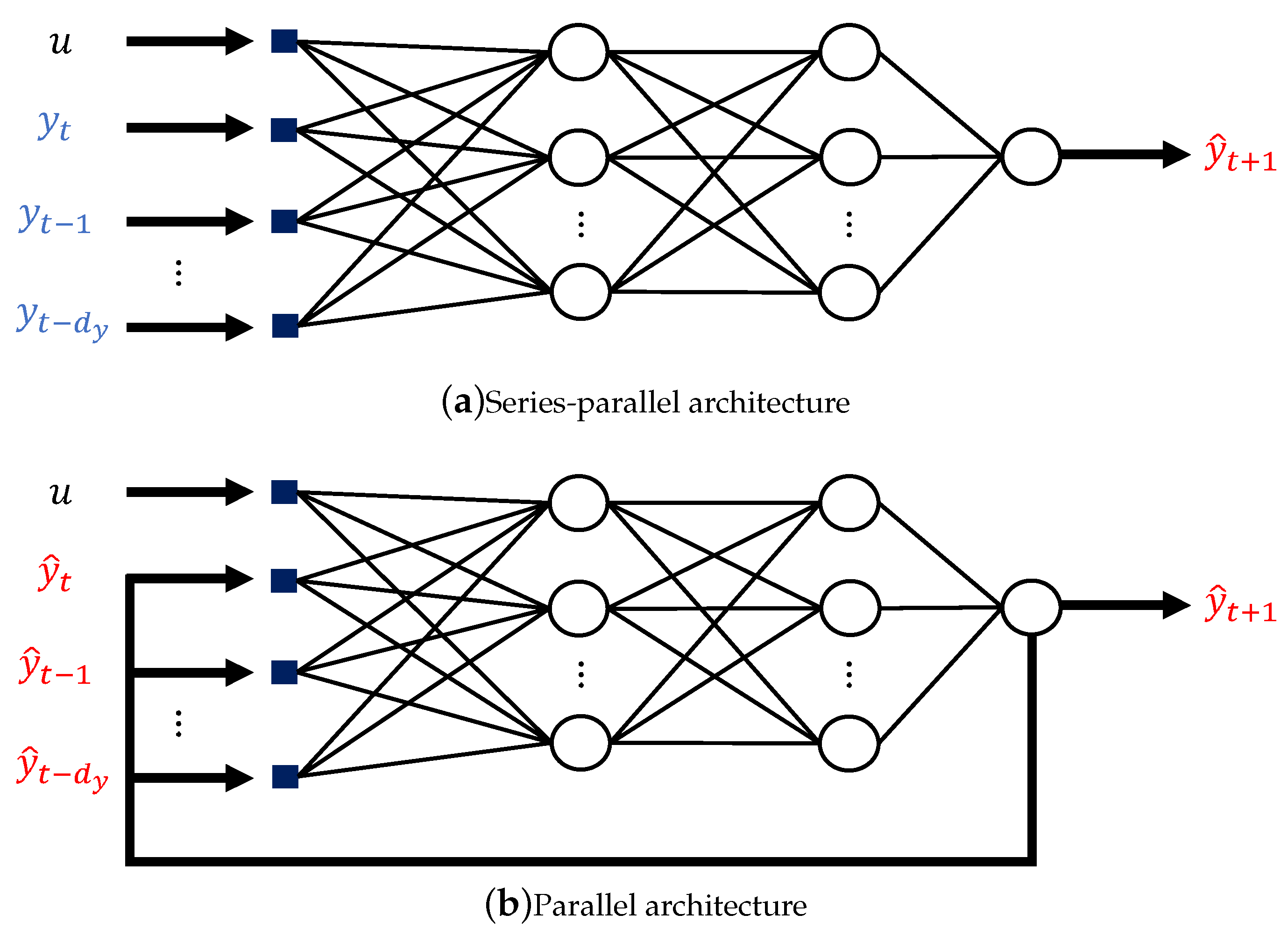
2.3. Aligning the ANN Structure with Physical Knowledge of the System

ANN representation via NARX has two different training architectures, namely Series-Parallel (SP) and Parallel (P) structure. The network output ${\widehat{\mathit{y}}}_{SP}\left(t+1\right)$ of the SP structure is a function of the observed target values of previous time steps $\mathit{y}\left(t\right)$ up to a feedback delay $d_y$ and of the so-called exogenous inputs $\mathit{u}$:

$${\widehat{\mathit{y}}}_{SP}\left(t+1\right)=f\left(\mathit{y}\left(t\right),\mathit{y}(t-1),\dots ,\mathit{y}(t-d_y),\mathit{u}\right).$$

(9)

In this work, $\mathit{u}$ was assumed to be constant over time, meaning there is no disturbance signal throughout the whole simulation period.

In P structure, the difference lies in the fed-back values. Here, the network outputs of the P structure ${\widehat{\mathit{y}}}_P\left(t\right)$ are fed-back instead of the original given data $\mathit{y}\left(t\right)$:

$${\widehat{\mathit{y}}}_P\left(t+1\right)=f\left(\widehat{\mathit{y}}\left(t\right),\widehat{\mathit{y}}(t-1),\dots ,\widehat{\mathit{y}}(t-d_y),\mathit{u}\right).$$

(10)

Note that, in terms of notation, the difference only lies in the hats above the fed-back values. Apparently, the P-structure in NARX resembles an explicit time-discrete differential equation (ODE or PDE) in a simplistic case, for example using the Adams–Bashforth discretization scheme [61,62] which can be described as:

$$\widehat{y}(t+1)\approx \widehat{y}\left(t\right)+\Delta t·g(u,\widehat{y}\left(t\right),\widehat{y}(t-1),\dots ,\widehat{y}(t-d_y)).$$

(11)

where $\widehat{y}\left(t+1\right)$ is an explicit function of $\widehat{y}\left(t\right)\dots \widehat{y}\left(t-d_y\right)$. In Equation (10), the NARX function $f\left(\widehat{\mathit{y}}\left(t\right),\widehat{\mathit{y}}(t-1),\dots ,\widehat{\mathit{y}}(t-d_y),\mathit{u}\right)$ can be seen as an approximation of $\widehat{y}\left(t\right)+\Delta t·g(u,\widehat{y}\left(t\right),\widehat{y}(t-1),\dots ,\widehat{y}(t-d_y))$ in Equation (11). Based on this reason, we propose to train using P-structure for solving dynamic problems whenever possible. Additionally, training in P-structure helps the network to learn that there is dependency between predicted values at different time steps. While both architectures were considered for NARX training, only P architecture was used for testing, as for longer-term forecasting, real data of previous time steps are not available [52]. For better understanding of the difference between P and SP, Figure 2 illustrates both architectures.

Feedback delay is also an important property, because Equations (2)–(4) are not elliptic, and hence there will be a time delay for the effect of input change to change the output. Because of this memory effect and its nonlinearity, we propose to use a deeper recurrence in NARX to enable the network to learn the system’s latency. In this work, feedback delay values $d_y$ ranging from 1 to 5 were tested to get the optimum value.

Additional to an appropriate ODE-like structure, the hyperbolic tangent (tanh) function was chosen as activation function within the neurons of NARX. Tanh is a nonlinear activation function (named tansig function in MATLAB [63]). Aside from the nonlinearity, this choice was driven by the assumption that all the input parameters and the targets depend on each other via smooth functions (differentiable). This knowledge results, among others, from the presence of a diffusion term in all relevant transport equations, and from the absence of shock waves in the solutions to Equations (2)–(4). Hence, for each hidden layer l as shown in Figure 2, the layer output ${\mathit{a}}^{\left[l\right]}$ is computed in the feedforward procedure described in:

$${\mathit{a}}^{\left[l\right]}=\tan \mathrm{h}({\mathit{w}}^{\left[l\right]}{\mathit{a}}^{[l-1]}+{\mathit{b}}^{\left[l\right]}).$$

(12)

For the output layer L, a linear function is assigned for scaling, leading to:

$${\widehat{\mathit{y}}}^{\left[L\right]}={\mathit{w}}^{\left[L\right]}{\mathit{a}}^{[L-1]}+{\mathit{b}}^{\left[L\right]}.$$

(13)

2.4. Physical Constraints in the Training Objective Function

As loss function for training, the most commonly used performance measure is a Mean Squared Error (MSE). Equation (14) shows the MSE for n training datasets (here, we use the subscript D for “data” to label the error term $E_D$ in the loss function as the data-related term):

$$E_D=\frac{1}{n.n_t}\sum _{i=1}^n\sum _{t=1}^{n_t}{(y_{i,t}-{\widehat{y}}_{i,t})}^2,$$

(14)

where $i=1\dots n$ indicates a specific sample in the training dataset and $t=1\dots n_t$ indicates a specific time step. However, using MSE alone in the loss function is not enough most of the time. The optimization problem to be solved in training is typically an ill-posed problem in many instances [30]. Thus, regularisation is required to prevent overfitting.

In this work, the L2 regularisation method was used to increase the generalisation capability of the ANN [64]. L2 regularisation is also known as weight decay or ridge regression [65]. The goal of L2 regularisation is to force the network to have small parameter values (choosing the simpler network over the more complex one). This effectively adds a soft constraint to the loss function to prevent the network from blindly fitting the possible noise in training datasets:

$$E_{\theta }=\frac{1}{N}\sum _{j=1}^N{\theta }_j^2,$$

(15)

where N is the total number of network parameters (weights and biases), and $\theta \in {\mathbb{R}}^N$ are the network parameters.

To improve the network prediction and the physical plausibility even more, known physical laws were inserted as part of the network regularisation:

$$E_{phy,k}=\frac{1}{n.n_t}\sum _{i=1}^n\sum _{t=1}^{n_t}{\left(e_{phy,i,t,k}\right)}^2,$$

(16)

where the subscript k identifies a specific physical law, for example a mole balance equation, and $e_{phy,i,t,k}$ is the physical error listed in

Table 1. Physical constraints in training: loss term used in Equation (16).

k	Equation: ${\mathit{e}}_{\mathit{phy},\mathit{i},\mathit{t},\mathit{k}}=\dots$
	Dehydration	Hydration
1	$e_{MB}(i,t)$
2	$e_{EB}(i,t)$
3	$ReLU(-{\widehat{\nu }}_{CaO}(i,t))$
4	$ReLU(-{\widehat{x}}_{H_{2}O}(i,t))$
5	$ReLU(\varphi +{\widehat{\nu }}_{CaO}(i,t)-1)$
6	$ReLU(\widehat{p}(i,t-1)-\widehat{p}(i,t))$	$ReLU(\widehat{p}(i,t)-\widehat{p}(i,t-1))$
7	$ReLU(\widehat{T}(i,t-1)-\widehat{T}(i,t))$	$ReLU(\widehat{T}(i,t)-\widehat{T}(i,t-1))$
8	$ReLU({\widehat{\nu }}_{CaO}(i,t-1)-{\widehat{\nu }}_{CaO}(i,t))$	$ReLU({\widehat{\nu }}_{CaO}(i,t)-{\widehat{\nu }}_{CaO}(i,t-1))$
9	$ReLU(\widehat{T}(i,t)-T_{in})$	$ReLU(T_{in}-\widehat{T}(i,t))$

. For example, the term $e_{phy,i,t,1}$ corresponds to the mole balance equation for dehydration/hydration. The mole balance equation used for this regularisation is the H₂O mole balance, because it has the most complete storage, flux and source/sink term (the solid components are assumed to be immobile, and N₂ is inert). The mole balance error can be written as:

$$e_{MB}(i,t)=n_{H_{2}O,out}(i,t)-n_{H_{2}O,in}+\Delta n_{H_{2}O,sto}(i,t)-\Delta n_{H_{2}O,q}(i,t),$$

(17)

where $n_{H_{2}O}$ is the molar amount of H₂O, the subscript $out$, $in$, $sto$ and q denote outflow, inflow, storage and source/sink term, respectively. The mole balance error was used as a contraint $e_{phy,i,t,1}$ and is equal to 0 if the mole balance is fulfilled. Putting this equation as a regularisation term penalises the network if the mole balance is not satisfied. Similarly, the corresponding energy balance equation also has to be fulfilled:

$$e_{EB}(i,t)=Q_{out}(i,t)-Q_{in}+\Delta Q_{sto}(i,t)-\Delta Q_q(i,t),$$

(18)

where Q is the energy in the system. It was used as a regularisation in $e_{phy,i,t,2}$. A more detailed derivation of the mole balance error $e_{phy,i,t,1}$ and the energy balance error $e_{phy,i,t,2}$ can be found in Appendix B.

Further relations of the form $\mathcal{F}\left(\widehat{y}\right)\le 0$ (monotonicity and non-negative values) were implemented using the Rectified Linear Units (ReLU) function, so that the physical error was then calculated with $e_{phy,i,t,k}=ReLU\left(\mathcal{F}\left(\widehat{y}\right)\right)$ [46]. The ReLU function returns 0 as output value for negative arguments and linearly increases for positive arguments. Hence, it punishes positive values in proportion to their magnitudes. Examples of these ReLU constraints are $e_{phy,i,t,3}$ through $e_{phy,i,t,13}$. They define non-negativity and monotonicity of the predicted target variables. For both dehydration and hydration process, negative fractional values ${\widehat{\nu }}_{CaO}$ and ${\widehat{x}}_{H_{2}O}$ are physically and mathematically impossible. Therefore, in $e_{phy,i,t,3}$ and $e_{phy,i,t,4}$, the network is punished for predicting negative values for these targets. Additionally, for both processes, $e_{phy,i,t,5}$ provides an additional constraint for ${\widehat{\nu }}_{CaO}$, to limit the amount of CaO volume in relation with the porosity (${\widehat{\nu }}_{CaO}\le 1-\varphi$). All these monotonicity assumptions originated from the fact that the system’s material parameters are considered to be constant throughout operation of the system. Therefore, the system’s behaviour should be monotonic and bounded in the specified aspects. Specific for the dehydration process, $\widehat{p}$, $\widehat{T}$ and ${\widehat{\nu }}_{CaO}$ are expected to not decrease throughout the simulation. This results in the corresponding monotonicity constraints $e_{phy,i,t,6}$ to $e_{phy,i,t,8}$. The system temperature must also be lower or equal to the injected temperature as constrained in $e_{phy,i,t,9}$, because the injected temperature is higher than the initial temperature. Specifically for the hydration process, the monotonicity constraints $e_{phy,i,t,6}$ to $e_{phy,i,t,9}$ for the dehydration process are reversed, because the hydration process is the reverse of the dehydration process.

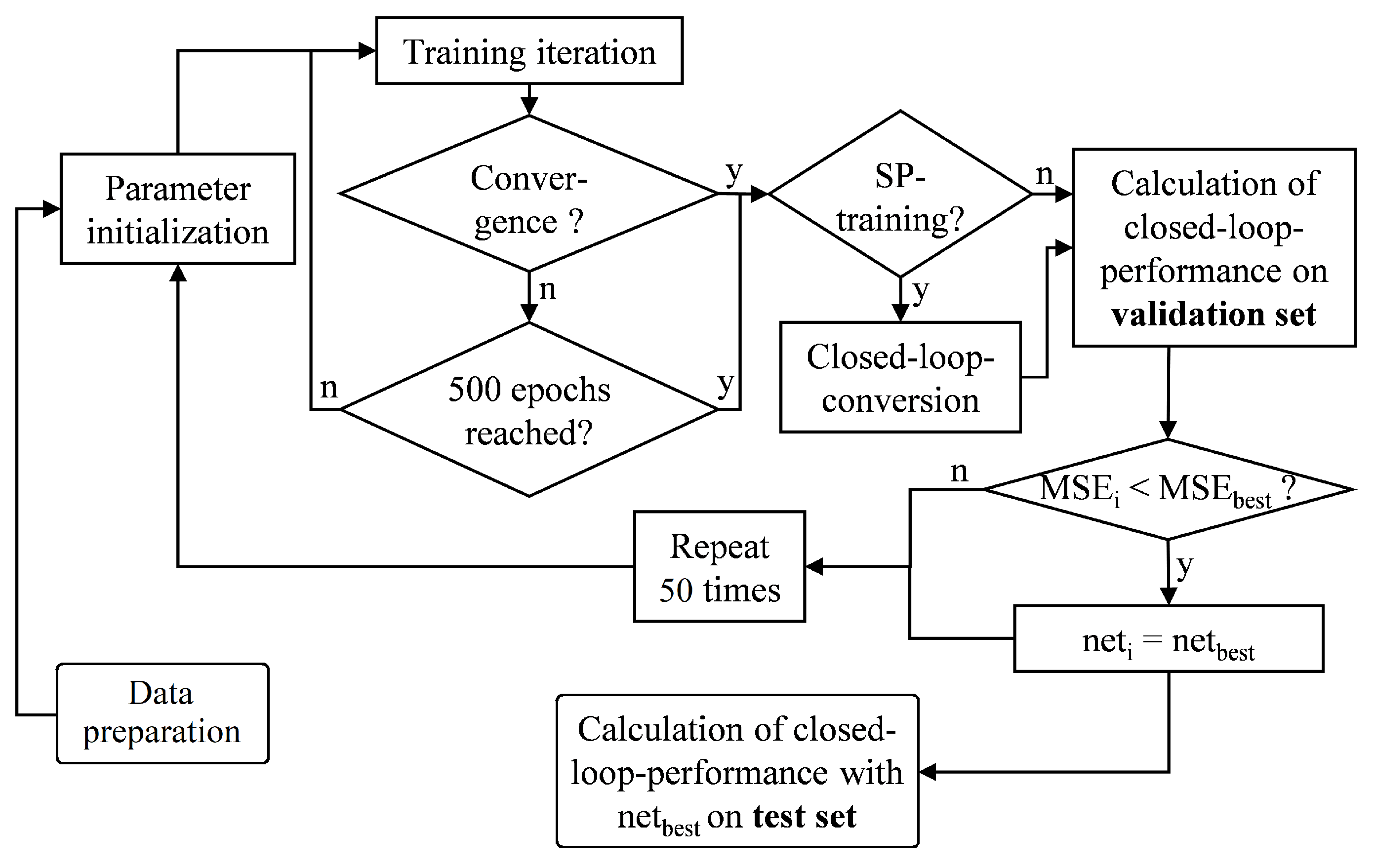
2.5. Obtaining Optimum Network Parameters

The complete loss function defined in Section 2.4 including MSE and all the regularisation term is written as:

$$L\left(\theta \right)=\alpha E_{\theta }+\beta E_D+\sum _k{\lambda }_k{E}_{phy,k}.$$

(19)

Here, $\alpha$ and $\beta$ are normalising constants of $E_{\theta }$ and $E_D$, respectively; and ${\lambda }_k$ is a normalising constant for each physical regularisation k. All error and regularisation terms, therefore, are evaluated in a normalised metric. These normalising constants, also known as the hyperparameters, determine the importance given to each term. For example, a high $\beta$ means that it is more important for the network to fit the training datasets than to generalise better. In many cases, the hyperparameters are determined manually from trial-and-error. In this work, Bayesian Regularisation was adopted to calculate them overall using a maximum likelihood approach to minimise $L\left(\theta \right)$ [66,67]. Bayesian Regularisation reduces the subjectivity arising from manual choice of hyperparameters. First, all the hyperparameters $\alpha$, $\beta$ and ${\lambda }_k$ along with the network parameters $\theta$ were initialised. The hyperparameters were initialised by setting $\beta =1$, $\alpha =0$ [68] and also ${\lambda }_k=0$, while the network parameters were initialised using the Nguyen-Widrow method [69,70]. The Nguyen-Widrow method initialises the network parameters so that each neuron contributes to a certain interval of the whole output range (added with some random values).

The complete derivation for updating $\alpha$ and $\beta$ can be found in [66,67]. Here, we only give the calculation of ${\lambda }_k$. After each iteration, they are updated according to the following relation:

$${\lambda }_k:=\frac{N-{\lambda }_{k}Trace\left({\mathit{H}}^{-1}{\mathit{J}}_{phy,k}^T{\mathit{J}}_{phy,k}\right)}{2E_{phy,k}},$$

(20)

where ${\mathit{J}}_{phy,k}$ is the Jacobian of physical error $E_{phy,k}$ with respect to the network parameters $\theta$. The approximate Hessian matrix $\mathit{H}$ of the overall loss function $L\left(\theta \right)$ was defined as follows:

$$\mathit{H}=\alpha \mathit{I}+\beta {\mathit{J}}_D^T{\mathit{J}}_D+\sum _k{\lambda }_k{\mathit{J}}_{phy,k}^T{\mathit{J}}_{phy,k},$$

(21)

where ${\mathit{J}}_D$ is the Jacobian of the MSE ($E_D$) with respect to the network parameters and $\mathit{I}$ is the $N\times N$ identity matrix (N is the number of network parameters $\theta$).

The network parameters are also updated after each iteration according to the Levenberg–Marquardt algorithm:

$$\theta :=\theta -{(\mathit{H}+\mathit{I}\mu )}^{-1}(\alpha \theta +\beta {\mathit{J}}_D{E}_D+\sum _k{\lambda }_k{\mathit{J}}_{phy,k}{E}_{phy,k}),$$

(22)

where $\mu >0$ is the algorithm’s damping parameter. Its value is increased when an iteration step is not successful, and is decreased otherwise. The Levenberg–Marquardt algorithm was chosen because of its faster convergence rate compared to Steepest Decent and higher stability relative to the Gauss–Newton algorithm [58]. In absence of our physical regularisation terms and with fixed $\alpha$, $\beta$, the procedure would simplify to a plain (nonlinear) least squares training, which would be the standard approach for training ANNs. Values of the trained network parameters and the normalising constants at the end of the training are given as supplementary materials on https://doi.org/10.18419/darus-634.

3. Results and Discussion

Our hypothesis is that applying physical knowledge of the modelled system into the construction of ANNs would lead to an improved physical plausibility of the prediction results. In this section, the prediction of the TCES system using ANNs is assessed and three relevant aspects that support our hypothesis are discussed: (I) the effect of feedback delay on the prediction result to account for the system’s nonlinearity and long-term memory effect (Section 3.1), (II) the comparison between training in SP and P architecture (Section 3.2) and (III) the improved physical plausibility from using physical regularisation (Section 3.3). The results are illustrated only for the dehydration process, because the hydration provides very similar results.

The complete workflow of the ANN application is shown in Figure 3. In general, the workflow can be divided into: training, validation and testing of the ANN. To train the ANN, first an ensemble of exogeneous input $\mathit{u}$ was generated based on selected probability distributions. These distributions are based on different values used in literature [6,17,18,19,20,21]. The complete list of exogeneous inputs $\mathit{u}$ with their corresponding distributions is listed in Appendix A. This ensemble was then plugged into the numerical model in DuMu^x and was simulated until $t=5000$ s to obtain an ensemble of target data $\mathit{y}\left(t\right)$. The governing equations are provided in Section 2.1. White noise was then added to these targets by generating normally distributed random numbers with zero mean and a standard deviation of 0.05 times the target values. Lastly, both exogenous inputs and targets were normalised to the range [−1, 1] to help the stability of the training [71]. Then, we set up the NARX ANN as described in Section 2. The training was then conducted using the built-in functions for NARX in the MATLAB Neural Network Toolbox [63], in which the loss function calculation was modified based on the equations provided in Section 2.5. It was conducted in batch mode both for dehydration and hydration process with a total of 100 training datasets.

Without physical regularisation, we obtain the lowest MSE value when the NARX is trained using 1000 training datasets, as shown in Figure 4. However, it is interesting to see how the physical knowledge can further improve the performance of NARX with limited training data. Therefore, we conducted the training in batch mode both for dehydration and hydration process with a total of only 100 training datasets.

For conciseness, the choice of the number of hidden layers, number of nodes per hidden layer and choice of activation function is not discussed because there is no existing uniform and systematic method to calculate the appropriate or the best combination [72]. Based on trial and error, we found that for this specific problem, 2 hidden layers with 15 and 8 nodes at each layer gives reasonable results. An example of ANN prediction using this configuration is provided in Appendix C. The stopping criteria are the dampening factor $\mathsf{\mu }>{10}^{10}$ (see Equation (22)) or the loss function gradient $g=\frac{\partial L\left(\theta \right)}{\partial \theta }<{10}^{-7}$, both of which are the default values proposed in the toolbox. Additionally, a maximum epochs is set for the training. Since training error converges mostly before 500 epochs, this limit is sufficient.

Different initialization values often lead to different network response as the algorithm might fail to always locate the global minimum [65]. Therefore, the network was retrained with 50 different initialisations. This number was set to find a compromise between a reliable result and a reasonable computational time. After each training, the network was validated on 20 validation datasets, and the trained network with the lowest MSE ($E_D$ evaluated against validation data) was selected. Finally, the network was tested with data contained neither in the training nor in the validation set on a test set with 800 time series.

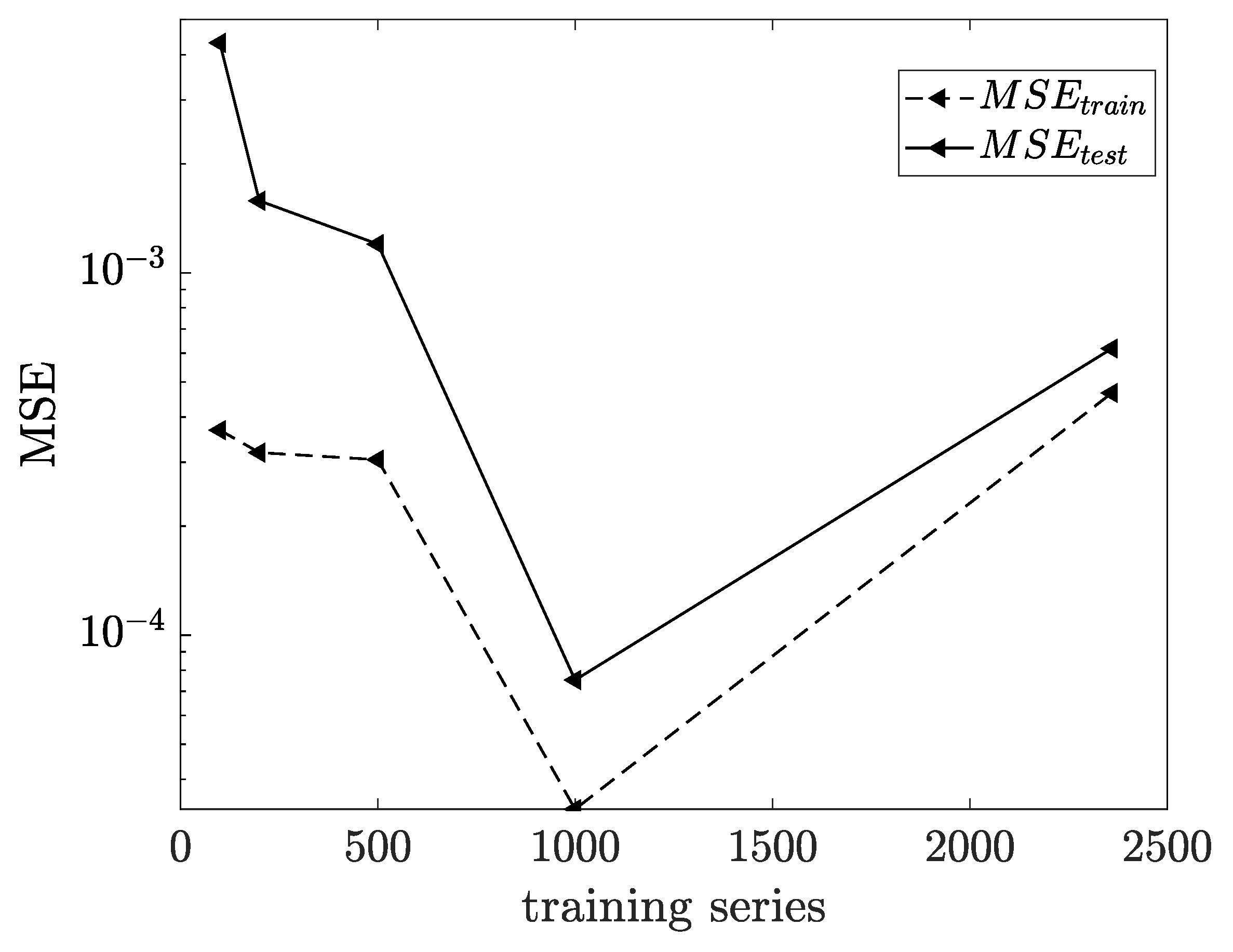
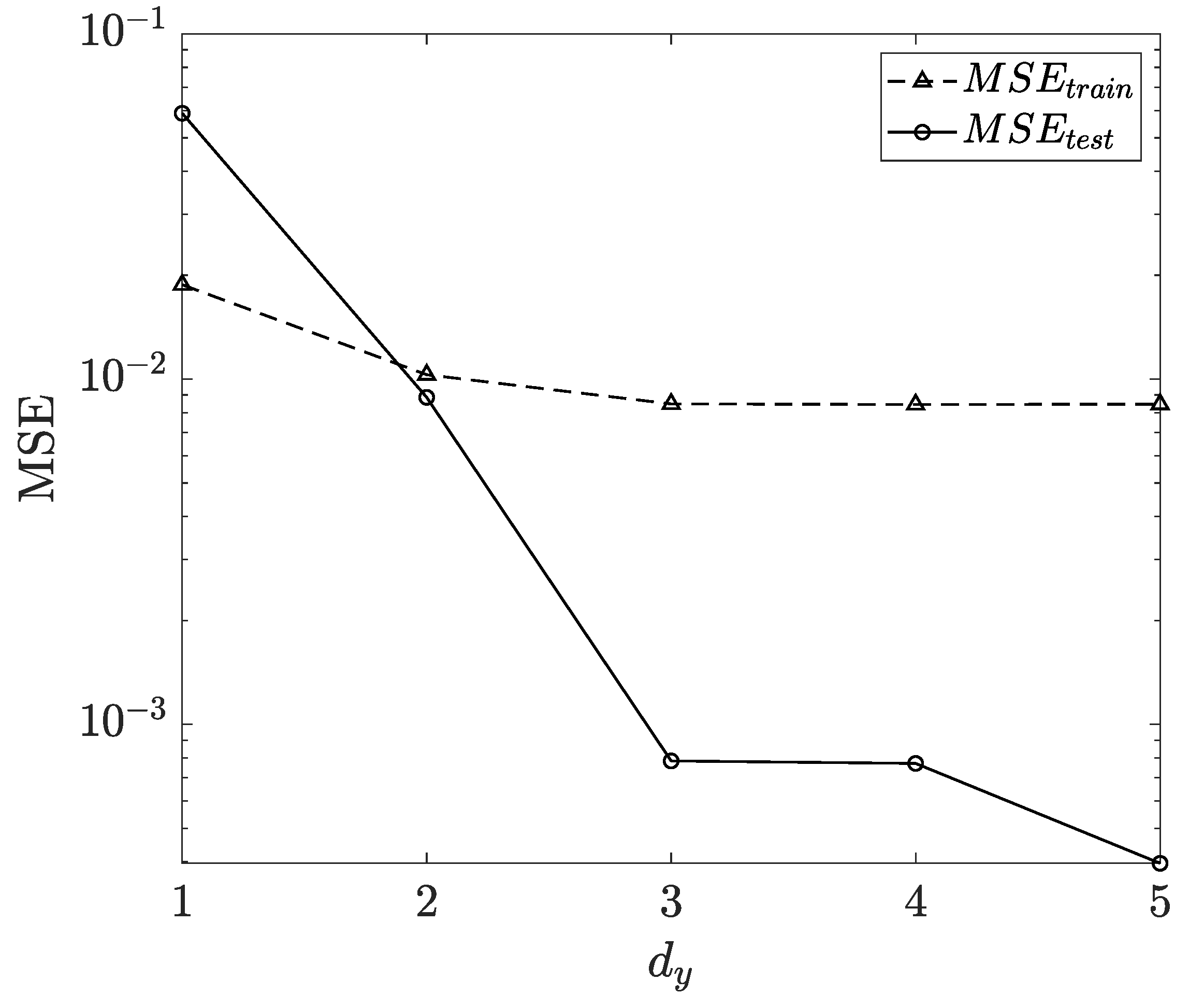
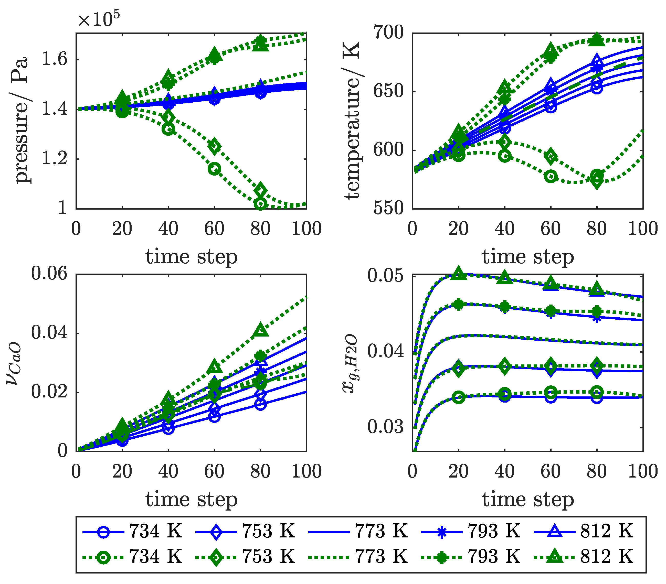
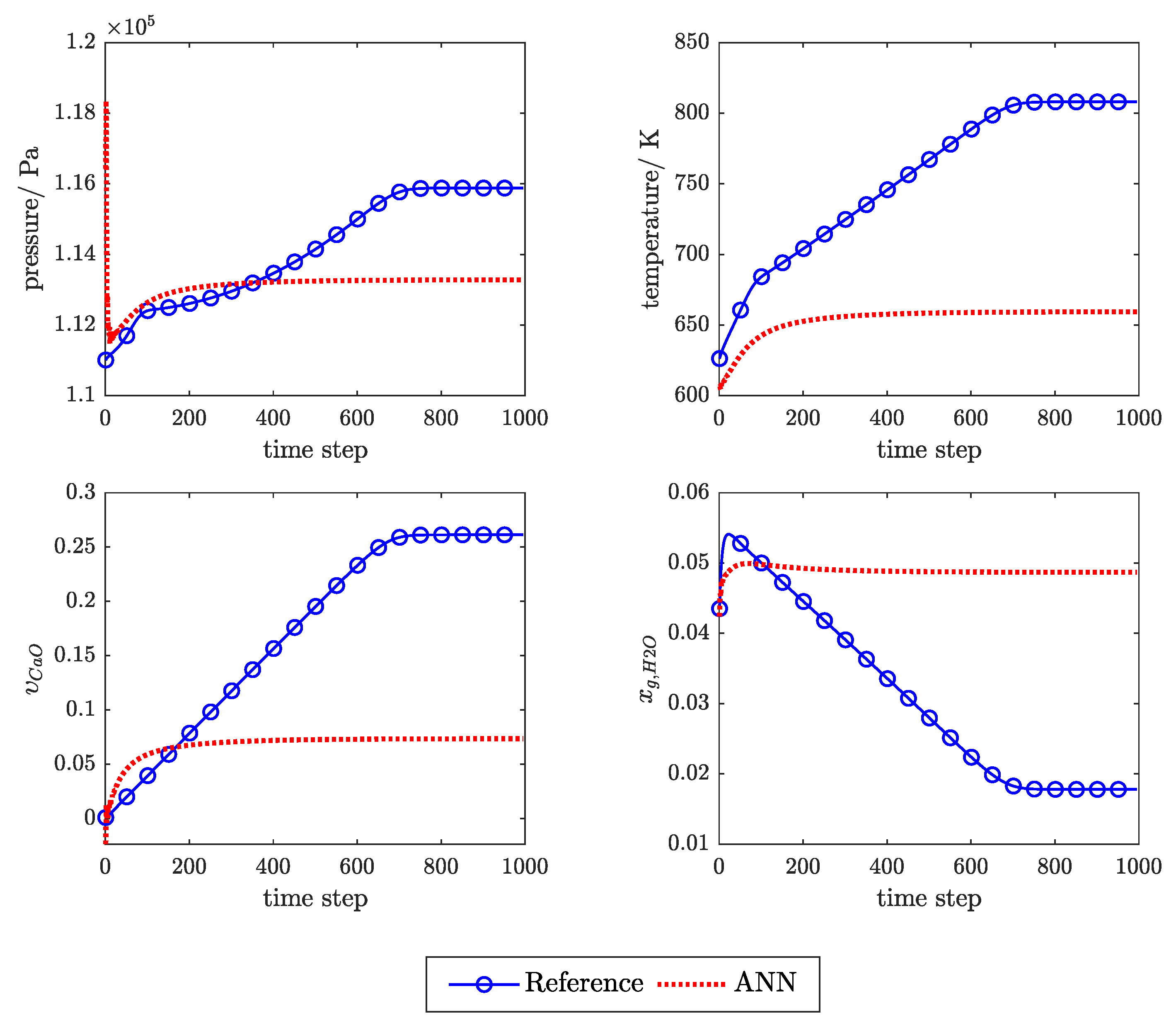
3.1. Influence of Feedback Delay

Figure 5 shows the influence of feedback delay on the MSE evaluated on both the training (dashed lines) and test datasets (solid lines) for networks trained using P structure. As shown in Figure 5, for $d_y>1$ the test MSE is lower than the training MSE. This is generally because the network was trained using additional white noise—producing more errors in the training, while the test datasets were smooth for reference.

In Figure 5, while the training error seems to remain constant at $d_y>2$, the test error keeps decreasing with increasing $d_y$. This clearly illustrates that including more depth in the recurrence improves the generalisation capability and therefore improves the ANN prediction. As the best $MS{E}_{test}$ was obtained with $d_y=5$, this value will be used from here onwards. From Figure 5 we can also analyse that a time delay of at least 3 previous time steps is useful to train the network. Moreover, we do not see the value of using $d_y>5$, as judging by the MSE trend in Figure 5, there is no significant improvement expected.

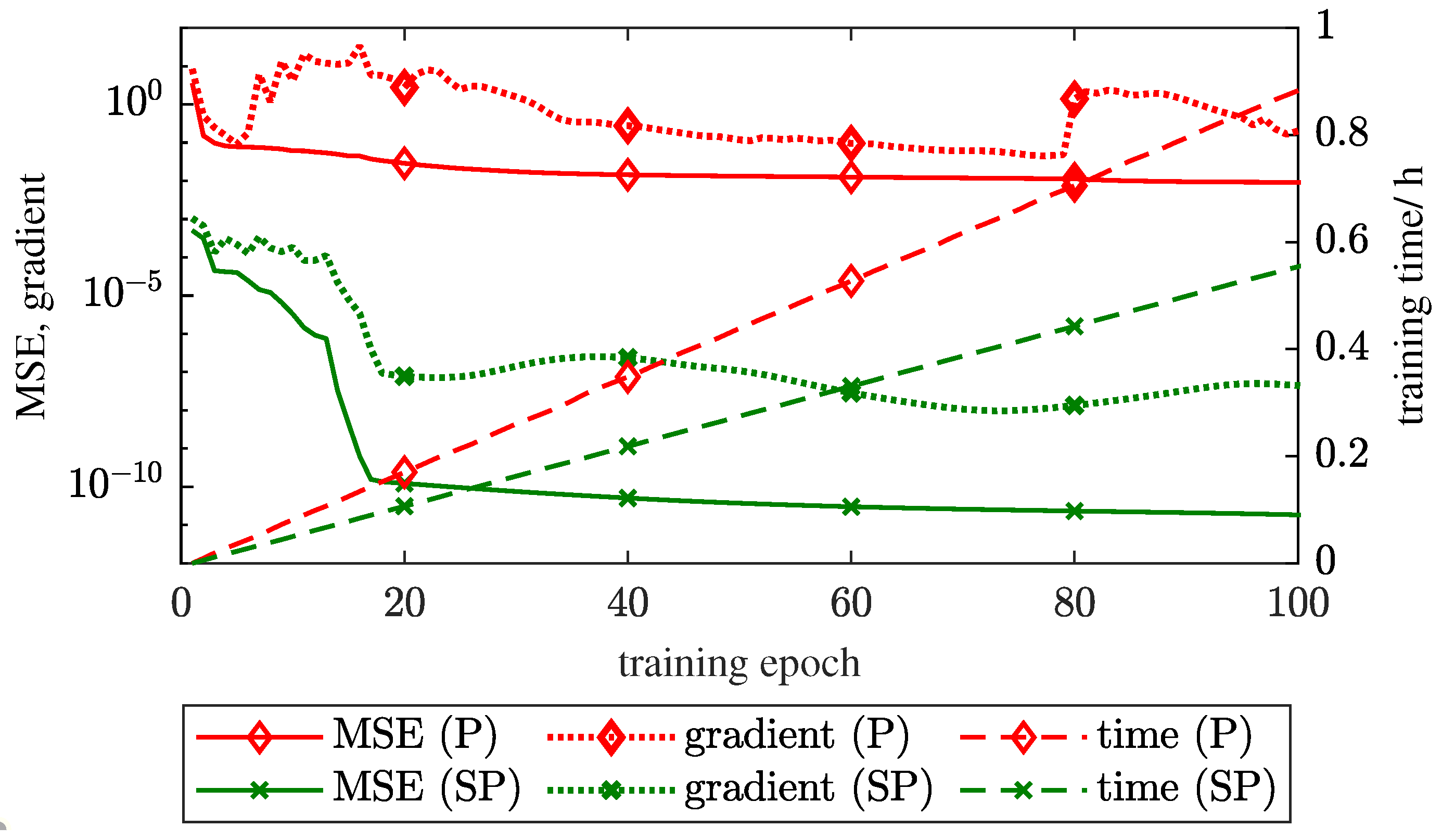
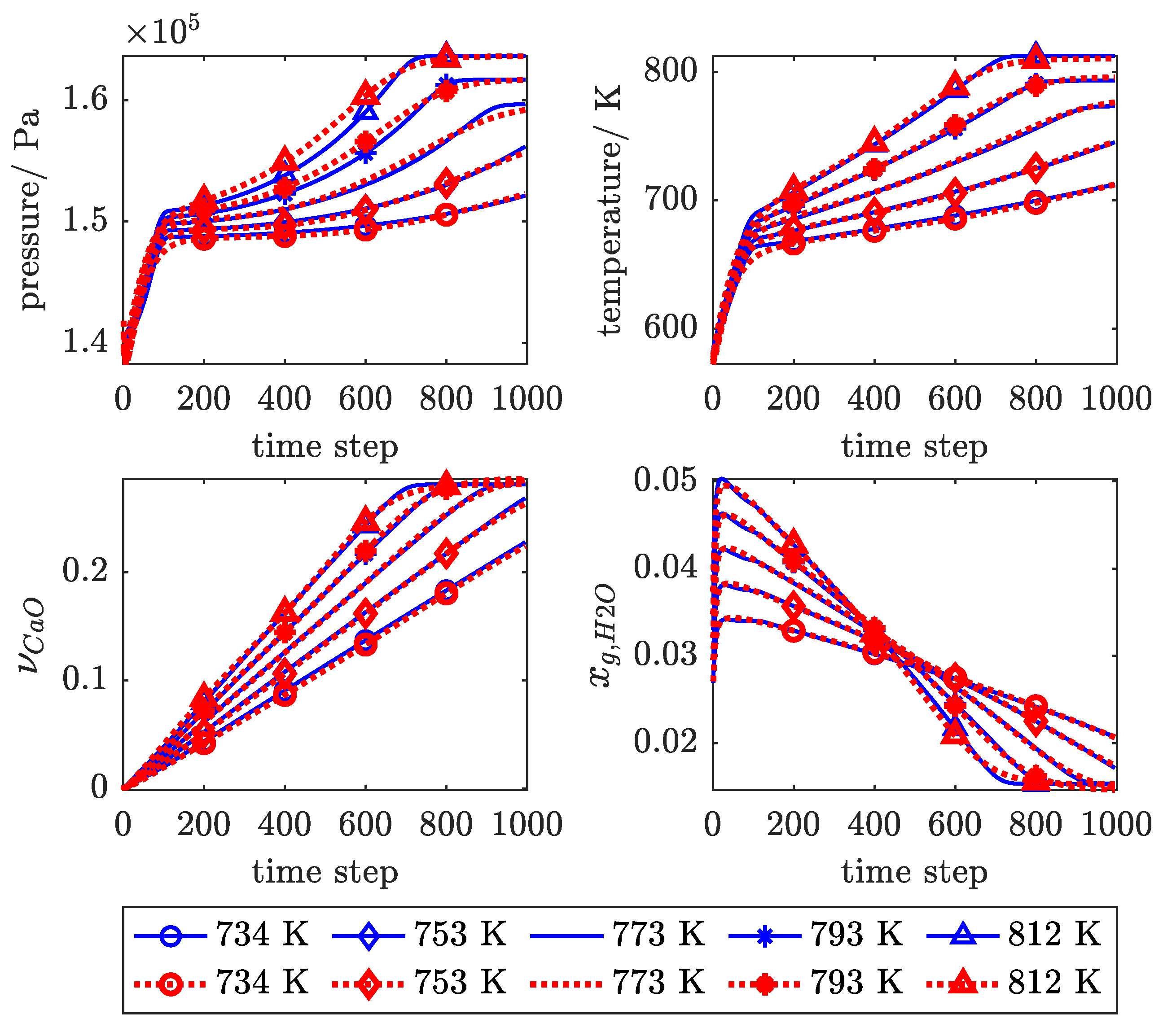
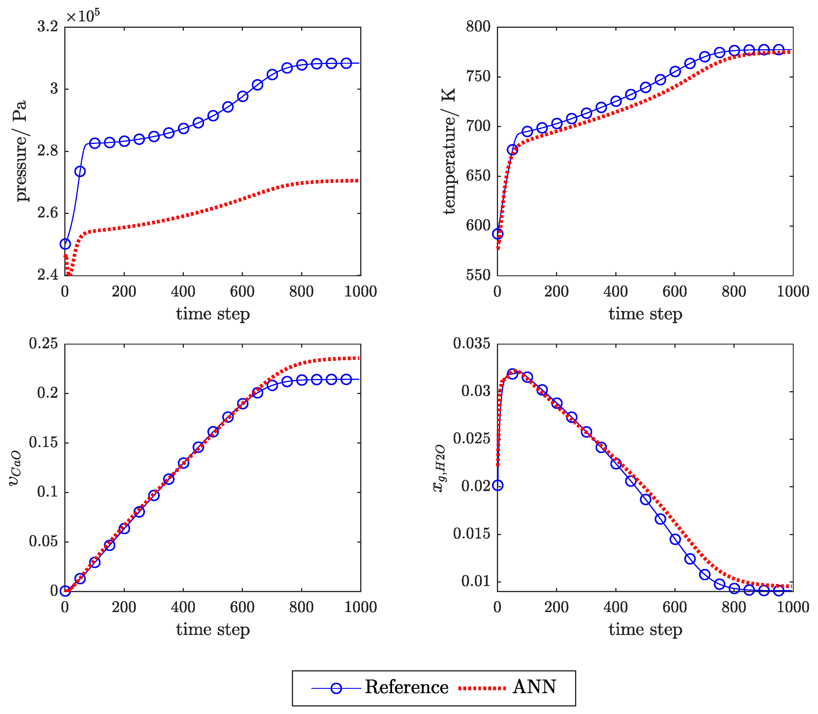
3.2. SP Versus P Training Structure

Figure 6 compares the training time of P compared to SP structure. Moreover, plotting the gradient and performance as function of training epochs allows us to analyse the difference between both training characteristics. As expected and shown in Figure 6 (dashed lines), both SP and P structure training time increases nearly linearly with the number of epochs (iterations). However, the slope is steeper for P training which is caused by higher computational cost using Backpropagation Through Time (BPTT).

In Recurrent ANNs, BPTT is used to calculate the derivative of the loss function instead of the normal backpropagation method. BPTT is technically the same as the normal backpropagation method but with the RNN unfolded through time being the main difference [30]. The gradient is then backpropagated through this unfolded network. Unfolding the recurrent network increases its size, and therefore the optimization problem becomes computationally more expensive and more difficult to solve.

After every epoch in P training, the output values change, and consequently the feedback values also change. The constantly changing feedback values cause additional changes of the gradient values along the iteration (dotted lines in Figure 6). This makes the training a more nonlinear problem. Correspondingly, the training performance (smaller MSE) increases much slower. In SP training, the gradient strongly decreases during the first 20 epochs, showing that the SP training is more computationally stable. However, the MSE (solid lines in Figure 6) was evaluated during training for the structure the network was trained with, meaning that the training performance does not consider the closed-loop conversion error for SP training. For that reason, the MSE values shown in Figure 6 seem to be better for SP training. Regardless of this difference, both training procedures converge with strictly monotonic decay of their MSE.

Next, the prediction performances of both training architectures are compared. In Figure 7, the results of the SP-trained NARX (dashed lines) are shown compared to the target values obtained from the simulation (solid lines) as reference solutions. Here, all target variables are calculated with differing inlet temperature. After a few time steps with relatively precise forecasts, the NARX predictions for T, p and ${\nu }_{CaO}$ diverge from real values and are highly fluctuating over time, which is nonphysical. Note that, in Figure 7, the results are shown only up to time step 100 instead of 1000. This is because the NARX prediction results after time step 100 have even higher fluctuations as the error propagates, hence making the comparison unclear visually. The forecast for $x_{g,H_{2}O}$ is reasonably accurate for $t<100$ but more erroneous for longer forecast periods. The forecast error is caused by the closed-loop-instability, meaning the inaccuracy caused by converting the network structure from SP to P. In other words, training using SP structure gives increasingly erroneous results with increasing time horizon. On the contrary, training with P structure provides clearly more accurate forecasts compared with SP, as shown in Figure 8. The NARX predictions (dotted lines) correspond really well to the reference targets (blue solid lines) throughout the whole simulation time for 1000 time steps, with inlet temperatures covering the whole range of its input distribution.

The comparison of P and SP structure shows that, while training in P structure seems to be more unstable, it provides significantly better long-term predictions because it trains the network to realise the time-dependency of output variables in a dynamic system. As shown by Equation (11), NARX resembles an explicitly discretized ODE, which is known to be conditionally stable. In cases where the discrete ODE is unstable, the error grows exponentially through time [73]. By training the network using P structure, the same structure is used for both training and testing, hence minimising the error propagation. The higher computing time needed to train in P structure (in comparison with training in SP structure) should not be a problem because the training only needs to be conducted once. Once the optimum network parameters are obtained, NARX can give reasonably accurate predictions with fast computational time. In fact, almost all studies in the area of surrogate models are willing to accept high computational costs during training (called offline costs) if the accuracy and speed for prediction (online) are good [54,74,75].

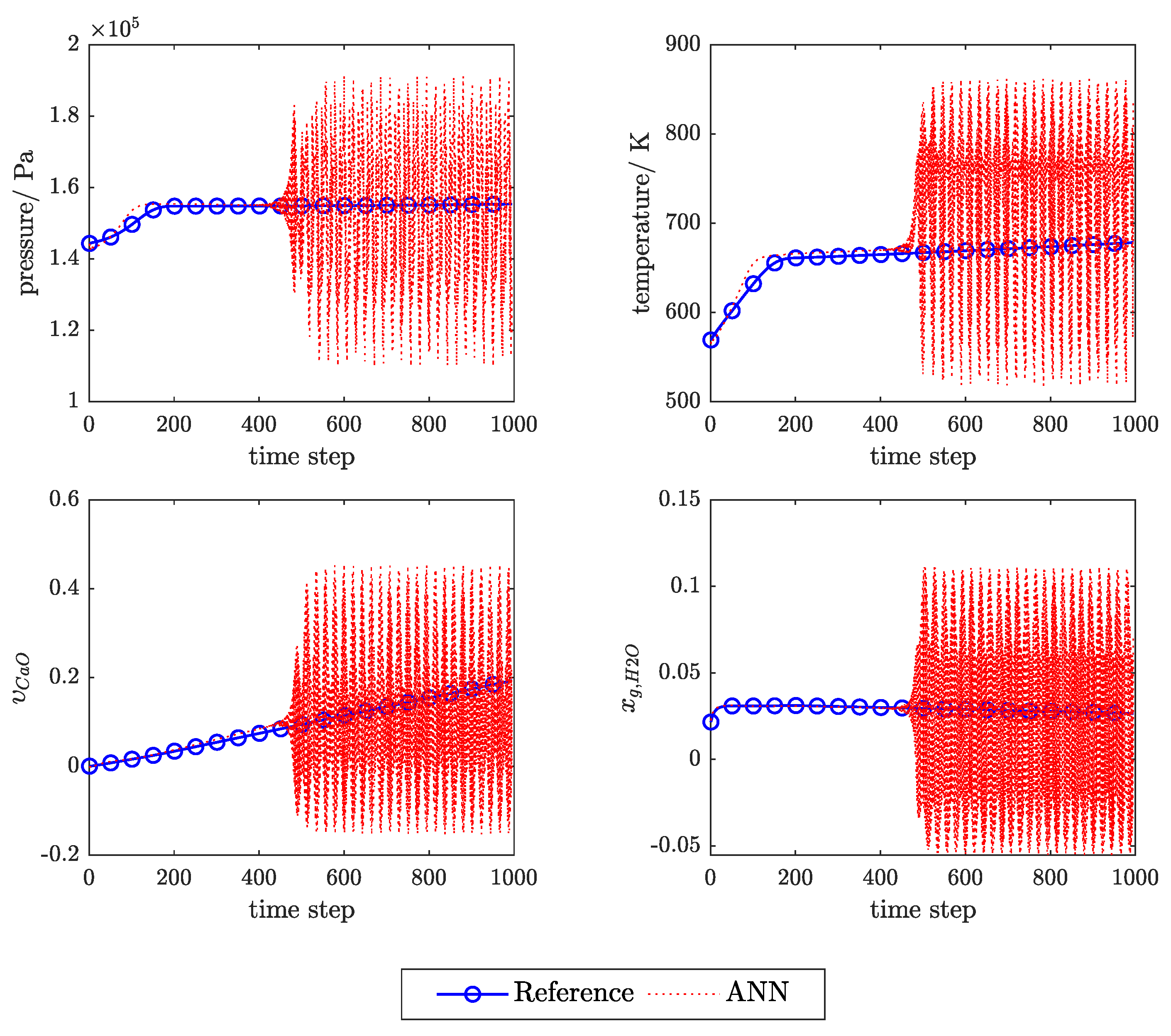
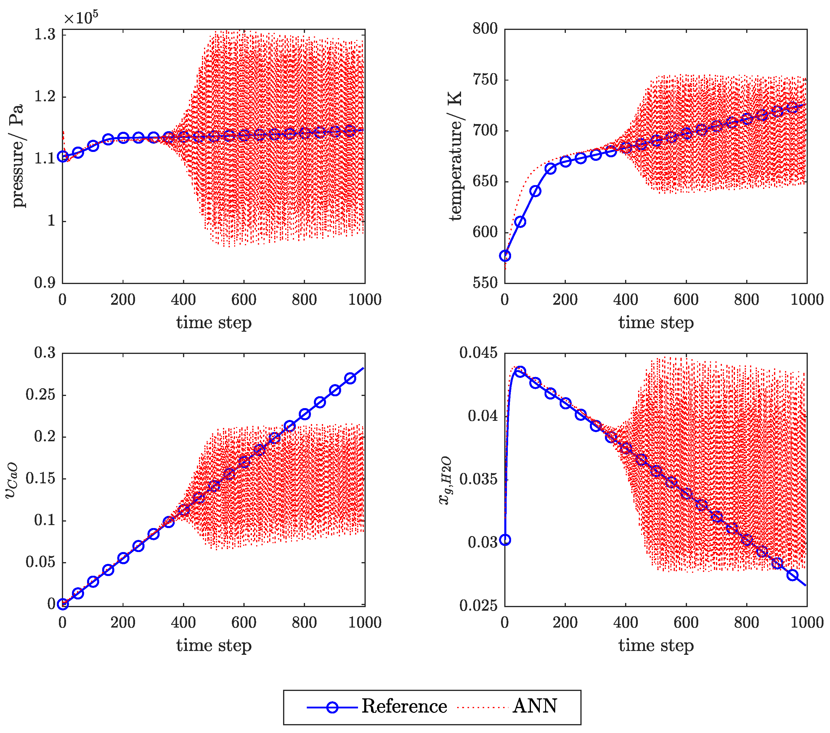
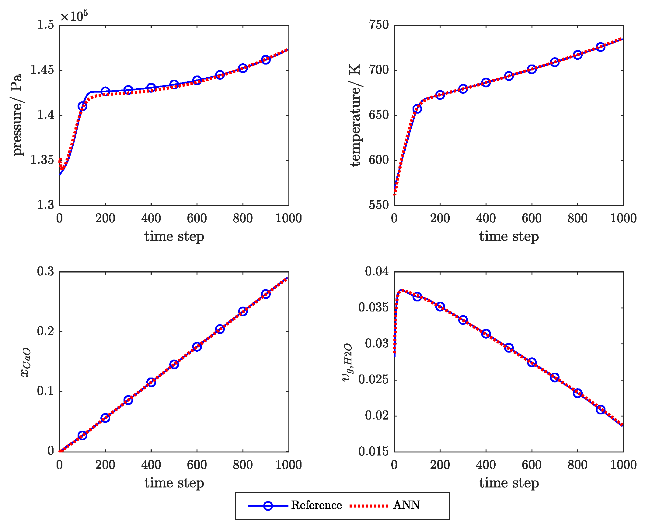
3.3. Physical Regularisation Improves Plausibility

To test the benefit of physically-based regularisation, the ANN performance is compared between training the network using:

• only MSE as the loss function (“MSE”), that is $L\left(\theta \right)=E_D$,
• MSE combined with only L2 (“MSE + L2”), that is $L\left(\theta \right)=\alpha E_{\theta }+\beta E_D$,
• MSE combined with only physical regularisation (“MSE + PHY”), that is $L\left(\theta \right)=\beta E_D+{\sum }_k{\lambda }_k{E}_{phy,k}$, and
• MSE combined with both L2 and physical regularisation (“MSE + L2 + PHY”), that is $L\left(\theta \right)=\alpha E_{\theta }+\beta E_D+{\sum }_k{\lambda }_k{E}_{phy,k}$.

To make a fair comparison, all networks were trained with the same set of initial network parameters. In this test, we used only P training and feedback delay $d_y=5$, because they clearly showed preferable performance in the previous sections. The comparison is summarised in

Table 2. MSE for different regularisation methods

Loss Function	${\mathit{MSE}}_{\mathit{train}}$	${\mathit{MSE}}_{\mathit{test}}$
MSE	$8.45\times {10}^{-3}$	$2.81\times {10}^{-3}$
MSE + L2	$9.01\times {10}^{-3}$	$3.96\times {10}^{-4}$
MSE + PHY	$8.68\times {10}^{-3}$	$3.83\times {10}^{-3}$
MSE + L2 + PHY	$8.43\times {10}^{-3}$	$3.96\times {10}^{-4}$

.

While the MSE on training data is in a comparable range for all loss functions, differences in $MS{E}_{test}$ are observed. L2 regularisation helps to reduce overfitting of training data, resulting in a lower test error in “MSE + L2” compared to “MSE”. At first glance, the additional physical regularisation does not seem to further improve the results. $MS{E}_{test}$ of “MSE + PHY” is slightly worse compared to “MSE”, and $MS{E}_{test}$ of “MSE + L2 + PHY” is in the same order with “MSE + L2” because another constraint is added in the objective function, while the performance is measured only based on MSE. Moreover, using only the physical (MSE + PHY) instead of only L2 regularisation (MSE + L2) leads to a test performance decrease.

Even though the performance for both “MSE” and “MSE + L2” are better than “MSE + PHY”, they both fail to produce physically plausible predictions in several test datasets (outliers) as shown in Figure 9 and Figure 10 (the label “Reference” for the blue line refers to the synthetic test data obtained from the physical model), the clearest one being negative fraction values of CaO and H₂O. One important aspect that needs to be considered is that the ANN was trained using only 100 training datasets, compared to almost 500 parameters that exist inside the network. This made the optimisation problem an ill-posed one, leading to clear overfitting in the network with “MSE” and “MSE + L2”. Physical regularisation tackles this problem even for relatively sparse training data, which is valuable once experiments are costly, and therefore, not much data are often available to train the network.

Even though it produces the worst overall test performance, physical regularisation alone (MSE + PHY) is able to produce physically plausible results despite no application of L2 regularisation, see Figure 11. The figure illustrates the worst prediction result of all test sets obtained using “MSE + PHY”. Even in its worst prediction with high error, the network is much more stable. With the addition of L2 regularisation in the “MSE + L2 + PHY” scheme, the prediction error (MSE) is further reduced so that it lies within the same range as “MSE + L2”. The major difference here is illustrated in Figure 12, where the worst prediction result produced by “MSE + L2 + PHY” is far more physically plausible, shown by the absence of unstable fluctuations as well as the relatively higher accuracy.

We trained the ANN using numerical simulation results which indirectly imbues the physics from the formulated governing equations into the ANN. When the ANN was not trained using numerical simulation results but with real observation data (which could follow more complex, scientifically unexplored equations), physical regularisation helps to constrain the ANN training at least to fundamental, confirmed laws and prevent unnecessary overfitting to the irregular and noisy observation data. As such, implementation of the method we present will be even more beneficial for applications with real observation data.

4. Conclusions

We adopted a PINN framework as an example of grey-box modelling to predict the dynamic internal states of the TCES system. Our approach aligns with the motivation of PINN that sees the modelled system as a complex unit that is underrepresented by the governing equations used in the physical model. We do not construct the ANN only as a surrogate model for the expensive numerical model, unlike in other PINN approaches that use ANN to infer the governing equations of the modelled system or the parameter values, assuming that the physical model describes the system perfectly. Our method was designed for application with real observation data that imply more complex processes than the simplified physical model. In this paper, however, we used synthetic data to train the ANN as a proof of concept.

As a key contribution, we propose to implement physical knowledge about a system into building the structure, choosing the training mode and designing the regularisation of ANNs to assure the physical plausibility and to increase the performance of the TCES dynamic internal state predictions. The alignment between the system’s behaviour (dynamic and nonlinear) and the ANN structure is described. The ANN predictions using different regularisation strategies are also compared to show the improvement provided by our method.

We show that, while training in P structure is computationally more expensive and unstable, the result is superior to training using SP structure, because P training resembles the dynamic of the governing differential equations better. Additionally, we found that, due to the nonlinearity and long-term memory effects implied by the system equations, deeper recurrency is necessary. A moderate depth of feedback delay produces better prediction performance, resulting from the network ability to capture the latency of the system. However, using too much feedback delay is also counter-productive, as it does not give significant improvement anymore, only increasing computational cost.

We also show that including physical regularisation to train the network improves the physical plausibility of the network predictions, even for worst-case scenarios. Physical regularisation helps the network to learn about relationships between different input and target variables, as well as the time-dependency between them. This includes mole and energy balance equations that serve as the building blocks of the system’s behaviour, along with simple monotonicity and non-negative constraints. However, physical regularisation alone is not enough to improve the generalisation capability of the network, and therefore, L2 regularisation is also necessary.

A very common issue with using ANNs in data-driven modelling is that obtaining experimental or operational data can be very costly, and therefore, there is often no sufficient data available to train the ANN. Our work shows that even with only a relatively small amount of training data (compared to the number of network parameters), using P training with a moderate amount of feedback delay $d_y$, combined with physical regularisation helps to prevent overfitting in optimising ill-posed problems and it produces relatively accurate and physically plausible predictions of the CaO/Ca(OH)₂ TCES system internal states. Further work is required for more sophisticated analysis of the system, for example with spatial distribution of the internal system, dynamic exogeneous input and uncertainty quantification of the predictions.

References

1. Haas, J.; Cebulla, F.; Cao, K.; Nowak, W.; Palma-Behnke, R.; Rahmann, C.; Mancarella, P. Challenges and trends of energy storage expansion planning for flexibility provision in power systems—A review. Renew. Sustain. Energy Rev. 2017, 80, 603–619. [Google Scholar] [CrossRef] [Green Version]
2. Møller, K.T.; Williamson, K.; Buckleyand, C.E.; Paskevicius, M. Thermochemical energy storage properties of a barium based reactive carbonate composite. J. Mater. Chem. 2020, 8, 10935–10942. [Google Scholar] [CrossRef]
3. Yuan, Y.; Li, Y.; Zhao, J. Development on Thermochemical Energy Storage Based on CaO-Based Materials: A Review. Sustainability 2018, 10, 2660. [Google Scholar] [CrossRef] [Green Version]
4. Pardo, P.; Deydier, A.; Anxionnaz-Minvielle, Z.; Rougé, S.; Cabassud, M.; Cognet, P. A review on high temperature thermochemical heat energy storage. Renew. Sustain. Energy Rev. 2014, 32, 591–610. [Google Scholar] [CrossRef] [Green Version]
5. Scapino, L.; Zondag, H.; Van Bael, J.; Diriken, J.; Rindt, C. Energy density and storage capacity cost comparison of conceptual solid and liquid sorption seasonal heat storage systems for low-temperature space heating. Renew. Sustain. Energy Rev. 2017, 76, 1314–1331. [Google Scholar] [CrossRef]
6. Schaube, F.; Wörner, A.; Tamme, R. High Temperature Thermochemical Heat Storage for Concentrated Solar Power Using Gas-Solid Reactions. J. Sol. Energy Eng. 2011, 133, 7. [Google Scholar] [CrossRef]
7. Carrillo, A.; Serrano, D.; Pizarro, P.; Coronado, J. Thermochemical heat storage based on the Mn2O3/Mn3O4 redox couple: Influence of the initial particle size on the morphological evolution and cyclability. J. Mater. Chem. 2014, 2, 19435–19443. [Google Scholar] [CrossRef]
8. Carrillo, A.; Moya, J.; Bayón, A.; Jana, P.; de la Peña O’Shea, V.; Romero, M.; Gonzalez-Aguilar, J.; Serrano, D.; Pizarro, P.; Coronado, J. Thermochemical energy storage at high temperature via redox cycles of Mn and Co oxides: Pure oxides versus mixed ones. Sol. Energy Mater. Sol. Cells 2014, 123, 47–57. [Google Scholar] [CrossRef]
9. Carrillo, A.; Sastre, D.; Serrano, D.; Pizarro, P.; Coronado, J. Revisiting the BaO2/BaO redox cycle for solar thermochemical energy storage. Phys. Chem. Chem. Phys. 2016, 18, 8039–8048. [Google Scholar] [CrossRef]
10. Muthusamy, J.P.; Calvet, N.; Shamim, T. Numerical Investigation of a Metal-oxide Reduction Reactor for Thermochemical Energy Storage and Solar Fuel Production. Energy Procedia 2014, 61, 2054–2057. [Google Scholar] [CrossRef] [Green Version]
11. Block, T.; Knoblauch, N.; Schmücker, M. The cobalt-oxide/iron-oxide binary system for use as high temperature thermochemical energy storage material. Thermochim. Acta 2014, 577, 25–32. [Google Scholar] [CrossRef]
12. Michel, B.; Mazet, N.; Neveu, P. Experimental investigation of an innovative thermochemical process operating with a hydrate salt and moist air for thermal storage of solar energy: Global performance. Appl. Energy 2014, 129, 177–186. [Google Scholar] [CrossRef] [Green Version]
13. Uchiyama, N.; Takasu, H.; Kato, Y. Cyclic durability of calcium carbonate materials for oxide/water thermo-chemical energy storage. Appl. Therm. Eng. 2019, 160, 113893. [Google Scholar] [CrossRef]
14. Yan, T.; Wang, R.; Li, T.; Wang, L.; Fred, I. A review of promising candidate reactions for chemical heat storage. Renew. Sustain. Energy Rev. 2015, 43, 13–31. [Google Scholar] [CrossRef]
15. Zhang, H.; Baeyens, J.; Cáceres, G.; Degréve, J.; Lv, Y. Thermal energy storage: Recent developments and practical aspects. Prog. Energy Combust. Sci. 2016, 53, 1–40. [Google Scholar] [CrossRef]
16. André, L.; Abanades, S.; Flamant, G. Screening of thermochemical systems based on solid-gas reversible reactions for high temperature solar thermal energy storage. Renew. Sustain. Energy Rev. 2016, 64, 703–715. [Google Scholar] [CrossRef]
17. Schaube, F.; Koch, L.; Wörner, A.; Müller-Steinhagen, H. A thermodynamic and kinetic study of the de- and rehydration of Ca(OH)2 at high H2O partial pressures for thermo-chemical heat storage. Thermochim. Acta 2012, 538, 9–20. [Google Scholar] [CrossRef]
18. Schaube, F.; Kohzer, A.; Schütz, J.; Wörner, A.; Müller-Steinhagen, H. De- and rehydration of Ca(OH)2 in a reactor with direct heat transfer for thermo-chemical heat storage. Part A: Experimental results. Chem. Eng. Res. Des. 2013, 91, 856–864. [Google Scholar] [CrossRef]
19. Schmidt, M.; Gutierrez, A.; Linder, M. Thermochemical energy storage with CaO/Ca(OH)2 - Experimental investigation of the thermal capability at low vapor pressures in a lab scale reactor. Appl. Energy 2017, 188, 672–681. [Google Scholar] [CrossRef]
20. Shao, H.; Nagel, T.; Roßkopf, C.; Linder, M.; Wörner, A.; Kolditz, O. Non-equilibrium thermo-chemical heat storage in porous media: Part 2—A 1D computational model for a calcium hydroxide reaction system. Energy 2013, 60, 271–282. [Google Scholar] [CrossRef]
21. Nagel, T.; Shao, H.; Roßkopf, C.; Linder, M.; Wörner, A.; Kolditz, O. The influence of gas-solid reaction kinetics in models of thermochemical heat storage under monotonic and cyclic loading. Appl. Energy 2014, 136, 289–302. [Google Scholar] [CrossRef]
22. Bayon, A.; Bader, R.; Jafarian, M.; Fedunik-Hofman, L.; Sun, Y.; Hinkley, J.; Miller, S.; Lipiński, W. Techno-economic assessment of solid–gas thermochemical energy storage systems for solar thermal power applications. Energy 2018, 149, 473–484. [Google Scholar] [CrossRef]
23. Rezvanizaniani, S.M.; Liu, Z.; Chen, Y.; Lee, J. Review and recent advances in battery health monitoring and prognostics technologies for electric vehicle (EV) safety and mobility. J. Power Sources 2014, 256, 110–124. [Google Scholar] [CrossRef]
24. Mehne, J.; Nowak, W. Improving temperature predictions for Li-ion batteries: Data assimilation with a stochastic extension of a physically-based, thermo-electrochemical model. J. Energy Storage 2017, 12, 288–296. [Google Scholar] [CrossRef]
25. Seitz, G.; Helmig, R.; Class, H. A numerical modeling study on the influence of porosity changes during thermochemical heat storage. Appl. Energy 2020, 259, 114152. [Google Scholar] [CrossRef]
26. Roßkopf, C.; Haas, M.; Faik, A.; Linder, M.; Wörner, A. Improving powder bed properties for thermochemical storage by adding nanoparticles. Energy Convers. Manag. 2014, 86, 93–98. [Google Scholar] [CrossRef]
27. Abiodun, O.I.; Jantan, A.; Omolara, A.E.; Dada, K.V.; Mohamed, N.A.; Arshad, H. State-of-the-art in artificial neural network applications: A survey. Heliyon 2018, 4, e00938. [Google Scholar] [CrossRef] [PubMed] [Green Version]
28. Raissi, M.; Perdikaris, P.; Karniadakis, G. Inferring solutions of differential equations using noisy multi-fidelity data. J. Comput. Phys. 2017, 335, 736–746. [Google Scholar] [CrossRef] [Green Version]
29. Karamizadeh, S.; Abdullah, S.M.; Halimi, M.; Shayan, J.J.; Rajabi, M. Advantage and drawback of support vector machine functionality. In Proceedings of the 2014 International Conference on Computer, Communications, and Control Technology (I4CT), Langkawi, Malaysia, 2–4 September 2014; pp. 63–65. [Google Scholar]
30. Aggarwal, C. Neural Networks and Deep Learning: A Textbook, 1st ed.; Springer: Cham, Switzerland, 2018. [Google Scholar]
31. Oyebode, O.; Stretch, D. Neural network modeling of hydrological systems: A review of implementation techniques. Nat. Resour. Model. 2018, 32, e12189. [Google Scholar] [CrossRef] [Green Version]
32. Chen, S.; Wang, Y.; Tsou, I. Using artificial neural network approach for modelling rainfall–runoff due to typhoon. J. Earth Syst. Sci. 2013, 122, 399–405. [Google Scholar] [CrossRef] [Green Version]
33. Asadi, H.; Shahedi, K.; Jarihani, B.; Sidle, R.C. Rainfall-Runoff Modelling Using Hydrological Connectivity Index and Artificial Neural Network Approach. Water 2019, 11, 212. [Google Scholar] [CrossRef] [Green Version]
34. Wunsch, A.; Liesch, T.; Broda, S. Forecasting groundwater levels using nonlinear autoregressive networks with exogenous input (NARX). J. Hydrol. 2018, 567, 743–758. [Google Scholar] [CrossRef]
35. Taherdangkoo, R.; Tatomir, A.; Taherdangkoo, M.; Qiu, P.; Sauter, M. Nonlinear Autoregressive Neural Networks to Predict Hydraulic Fracturing Fluid Leakage into Shallow Groundwater. Water 2020, 12, 841. [Google Scholar] [CrossRef] [Green Version]
36. Kalogirou, S. Applications of artificial neural-networks for energy systems. Appl. Energy 1995, 67, 17–35. [Google Scholar] [CrossRef]
37. Bermejo, J.; Fernández, J.; Polo, F.; Márquez, A. A Review of the Use of Artificial Neural Network Models for Energy and Reliability Prediction. A Study of the Solar PV, Hydraulic and Wind Energy Sources. Appl. Sci. 2019, 9, 1844. [Google Scholar] [CrossRef] [Green Version]
38. Yaïci, W.; Entchev, E.; Longo, M.; Brenna, M.; Foiadelli, F. Artificial neural network modelling for performance prediction of solar energy system. In Proceedings of the 2015 International Conference on Renewable Energy Research and Applications (ICRERA), Palermo, Italy, 22–25 November 2015; pp. 1147–1151. [Google Scholar]
39. Kumar, A.; Zaman, M.; Goel, N.; Srivastava, V. Renewable Energy System Design by Artificial Neural Network Simulation Approach. In Proceedings of the 2014 IEEE Electrical Power and Energy Conference, Calgary, AB, Canada, 12–14 November 2014; pp. 142–147. [Google Scholar]
40. Breiman, L. Statistical Modeling: The Two Cultures. Stat. Sci. 2001, 16, 199–231. [Google Scholar] [CrossRef]
41. Zhang, Z.; Beck, M.W.; Winkler, D.A.; Huang, B.; Sibanda, W.; Goyal, H. Opening the black box of neural networks: Methods for interpreting neural network models in clinical applications. Ann. Transl. Med. 2018, 6, 1–11. [Google Scholar] [CrossRef]
42. Raissi, M.; Perdikaris, P.; Karniadakis, G.E. Physics Informed Deep Learning (Part I): Data-driven Solutions of Nonlinear Partial Differential Equations. arXiv 2017, arXiv:1711.10561. [Google Scholar]
43. Raissi, M.; Perdikaris, P.; Karniadakis, G.E. Physics Informed Deep Learning (Part II): Data-driven Discovery of Nonlinear Partial Differential Equations. arXiv 2017, arXiv:1711.10566. [Google Scholar]
44. Doshi-Velez, F.; Kim, B. Towards A Rigorous Science of Interpretable Machine Learning. arXiv 2017, arXiv:1702.08608v2. [Google Scholar]
45. Miller, T. Explanation in Artificial Intelligence: Insights from the Social Sciences. arXiv 2017, arXiv:1706.07269. [Google Scholar] [CrossRef]
46. Karpatne, A.; Atluri, G.; Faghmous, J.; Steinbach, M.; Banerjee, A.; Ganguly, A.; Shekhar, S.; Samatova, N.; Kumar, V. Theory-guided Data Science: A New Paradigm for Scientific Discovery from Data. arXiv 2017, arXiv:1612.08544v2. [Google Scholar] [CrossRef]
47. Tartakovsky, A.; Marrero, C.; Perdikaris, P.; Tartakovsky, G.; Barajas-Solano, D. Learning Parameters and Constitutive Relationships with Physics Informed Deep Neural Networks. arXiv 2018, arXiv:1808.03398v2. [Google Scholar]
48. Karpatne, A.; Watkins, W.; Read, J.; Kumar, V. Physics-guided Neural Networks (PGNN): An Application in Lake Temperature Modeling. arXiv 2018, arXiv:1710.11431v2. [Google Scholar]
49. Wang, N.; Zhang, D.; Chang, H.; Li, H. Deep learning of subsurface flow via theory-guided neural network. J. Hydrol. 2020, 584, 124700. [Google Scholar] [CrossRef] [Green Version]
50. Chen, S.; Billings, S.; Grant, P. Non-linear system identification using neural networks. Int. J. Control 1990, 51, 1191–1214. [Google Scholar] [CrossRef]
51. Zhang, X. Time series analysis and prediction by neural networks. Optim. Methods Softw. 1994, 4, 151–170. [Google Scholar] [CrossRef]
52. Buitrago, J.; Asfour, S. Short-Term Forecasting of Electric Loads Using Nonlinear Autoregressive Artificial Neural Networks with Exogenous Vector Inputs. Energies 2017, 10, 40. [Google Scholar] [CrossRef] [Green Version]
53. Boussaada, Z.; Curea, O.; Remaci, A.; Camblong, H.; Bellaaj, N. A Nonlinear Autoregressive Exogenous (NARX) Neural Network Model for the Prediction of the Daily Direct Solar Radiation. Energies 2018, 11, 620. [Google Scholar] [CrossRef] [Green Version]
54. Mellit, A.; Kalogirou, S. Artificial intelligence techniques for photovoltaic applications: A review. Prog. Energy Combust. Sci. 2008, 34, 574–632. [Google Scholar] [CrossRef]
55. Jia, X.; Karpatne, A.; Willard, J.; Steinbach, M.; Read, J.; Hanson, P.; Dugan, H.; Kumar, V. Physics Guided Recurrent Neural Networks For Modeling Dynamical Systems: Application to Monitoring Water Temperature And Quality In Lakes. arXiv 2018, arXiv:1810.02880. [Google Scholar]
56. Levenberg, K. A method for the solution of certain non-linear problems in least squares. Q. Appl. Math. 1944, 2, 164–168. [Google Scholar] [CrossRef] [Green Version]
57. Marquardt, D. An Algorithm for Least-Squares Estimation of Nonlinear Parameters. J. Soc. Ind. Appl. Math. 1963, 11, 431–441. [Google Scholar] [CrossRef]
58. Yu, H.; Wilamowski, B.M. Levenberg-Marquardt Training. In The Industrial Electronics Handbook—Intelligent Systems, 2nd ed.; Wilamowski, B., Irwin, J., Eds.; CRC Press: Boca Raton, FL, USA, 2011; Volume 5, Chapter 12. [Google Scholar]
59. Banerjee, I. Modeling Fractures in a CaO/Ca(OH)2 Thermo-chemical Heat Storage Reactor. Master’s Thesis, Universität Stuttgart, Stuttgart, Germany, 2018. [Google Scholar]
60. Koch, T.; Gläser, D.; Weishaupt, K.; Ackermann, S.; Beck, M.; Becker, B.; Burbulla, S.; Class, H.; Coltman, E.; Fetzer, T.; et al. Release 3.0.0 of DuMux: DUNE for Multi-{Phase, Component, Scale, Physics,...} Flow and Transport in Porous Media; Zenodo: Geneva, Switzerland, 2019. [Google Scholar] [CrossRef]
61. Peinado, J.; Ibáñez, J.; Arias, E.; Hernández, V. Adams-Bashforth and Adams-Moulton methods for solving differential Riccati equations. Comput. Math. Appl. 2010, 60, 3032–3045. [Google Scholar] [CrossRef] [Green Version]
62. Tutueva, A.; Karimov, T.; Butusov, D. Semi-Implicit and Semi-Explicit Adams-Bashforth-Moulton Methods. Mathematics 2020, 8, 780. [Google Scholar] [CrossRef]
63. Beale, M.; Hagan, M.; Demuth, H. Deep Learning Toolbox™ User’s Guide (R2019a); The MathWorks, Inc.: Natick, MA, USA, 2019. [Google Scholar]
64. Krogh, A.; Hertz, J.A. A Simple Weight Decay Can Improve Generalization. In Advances in Neural Information Processing Systems 4; Moody, J.E., Hanson, S.J., Lippmann, R.P., Eds.; Morgan-Kaufmann: Denver, CO, USA, 1991; pp. 950–957. [Google Scholar]
65. Goodfellow, I.; Bengio, Y.; Courville, A. Deep Learning; MIT Press: Cambridge, MA, USA, 2016; Available online: http://www.deeplearningbook.org (accessed on 15 April 2019).
66. MacKay, D. Bayesian Interpolation. Neural Comput. 1991, 4, 415–447. [Google Scholar] [CrossRef]
67. Sariev, E.; Germano, G. Bayesian regularized artificial neural networks for the estimation of the probability of default. Quant. Financ. 2020, 20, 311–328. [Google Scholar] [CrossRef]
68. Foresee, F.D.; Hagan, M. Gauss-Newton approximation to Bayesian learning. IEEE 1997, 3, 1930–1935. [Google Scholar] [CrossRef]
69. Nguyen, D.; Widrow, B. Improving the learning speed of 2-layer neural networks by choosing initial values of the adaptive weights. IEEE 1990, 3, 21–26. [Google Scholar] [CrossRef]
70. Mittal, A.; Singh, A.P.; Chandra, P. A Modification to the Nguyen–Widrow Weight Initialization Method. In Intelligent Systems, Technologies and Applications; Springer: Singapore, 2020; pp. 141–153. [Google Scholar]
71. Zhang, G.; Patuwo, B.E.; Hu, M. Forecasting with artificial neural networks: The state of the art. Int. J. Forecast. 1998, 14, 35–62. [Google Scholar] [CrossRef]
72. Stathakis, D. Adams-Bashforth and Adams-Moulton methods for solving differential Riccati equations. Int. J. Remote Sens. 2009, 30, 2133–2147. [Google Scholar] [CrossRef]
73. Higham, D.J.; Trefethen, L.N. Stiffness of ODEs. BIT Numer. Math. 1993, 33, 285–303. [Google Scholar] [CrossRef]
74. Härter, F.P.; de Campos Velho, H.F.; Rempel, E.L.; Chian, A.C.L. Neural networks in auroral data assimilation. J. Atmos. Sol.-Terr. Phys. 2008, 70, 1243–1250. [Google Scholar] [CrossRef]
75. Awolusi, T.F.; Oke, O.L.; Akinkurolere, O.O.; Sojobi, A.O.; Aluko, O.G. Performance comparison of neural network training algorithms in the modeling properties of steel fiber reinforced concrete. Heliyon 2019, 5, 1–27. [Google Scholar] [CrossRef] [Green Version]
Figure 1. A simplified schematic of a Thermochemical Energy Storage (TCES) system with CaO/Ca(OH)2 as the storage material during (a) dehydration and (b) hydration process.
Energies 13 03873 g001
Figure 2. Difference between (a) SP and (b) P architecture. Here, y t y t d y (in blue) are the given data, while y ^ t y ^ t d y (in red) are the ANN predictions.
Energies 13 03873 g002
Figure 3. Flowchart of training, validation and test of the ANN.
Energies 13 03873 g003
Figure 4. Comparison of MSE using different number of training datasets.
Energies 13 03873 g004
Figure 5. Feedback delay variation.
Energies 13 03873 g005
Figure 6. Training time, gradient and performance for P (Parallel) and SP (Series-Parallel) structure.
Energies 13 03873 g006
Figure 7. Forecasts with SP-trained NARX for various inlet temperatures.
Energies 13 03873 g007
Figure 8. Forecasts with P-trained NARX for various inlet temperatures.
Energies 13 03873 g008
Figure 9. Worst prediction sample (red) obtained with “Mean Squared Error—MSE” regularisation method and reference solution obtained from the physical model (blue).
Energies 13 03873 g009
Figure 10. Worst prediction sample (red) obtained with “MSE + L2” regularisation method and reference solution obtained from the physical model (blue).
Energies 13 03873 g010
Figure 11. Worst prediction sample (red) obtained with “MSE + PHY” regularisation method and reference solution obtained from the physical model (blue).
Energies 13 03873 g011
Figure 12. Worst prediction sample (red) obtained with “MSE + L2 + PHY” regularisation method and reference solution obtained from the physical model (blue).
Energies 13 03873 g012