Localized Convolutional Neural Networks for Geospatial Wind Forecasting


Abstract
:1. Introduction
2. Localized CNN Motivation
- The total amount of different trainable weights is drastically reduced, thus the model is:
- –
- Much less prone to overfitting;
- –
- Much smaller to store and often faster to train and run;
- Every filter is trained on every patch of every input image , which utilizes the training data well;
- The architecture and learned weights of the convolutional layer do not depend on the size of the input image, making them easier to reuse;
- Convolutions give translation invariance: the features are detected the same way, no matter where they are in the image.
- The explicit coordinates of each location like in CoordConv [5];
- A combination of local random static location-dependent inputs, that could potentially allow us to uniquely “identify” each location as well;
- The above mentioned real-world relevant unique location-specific features if they are explicitly available (typically not all of them are).
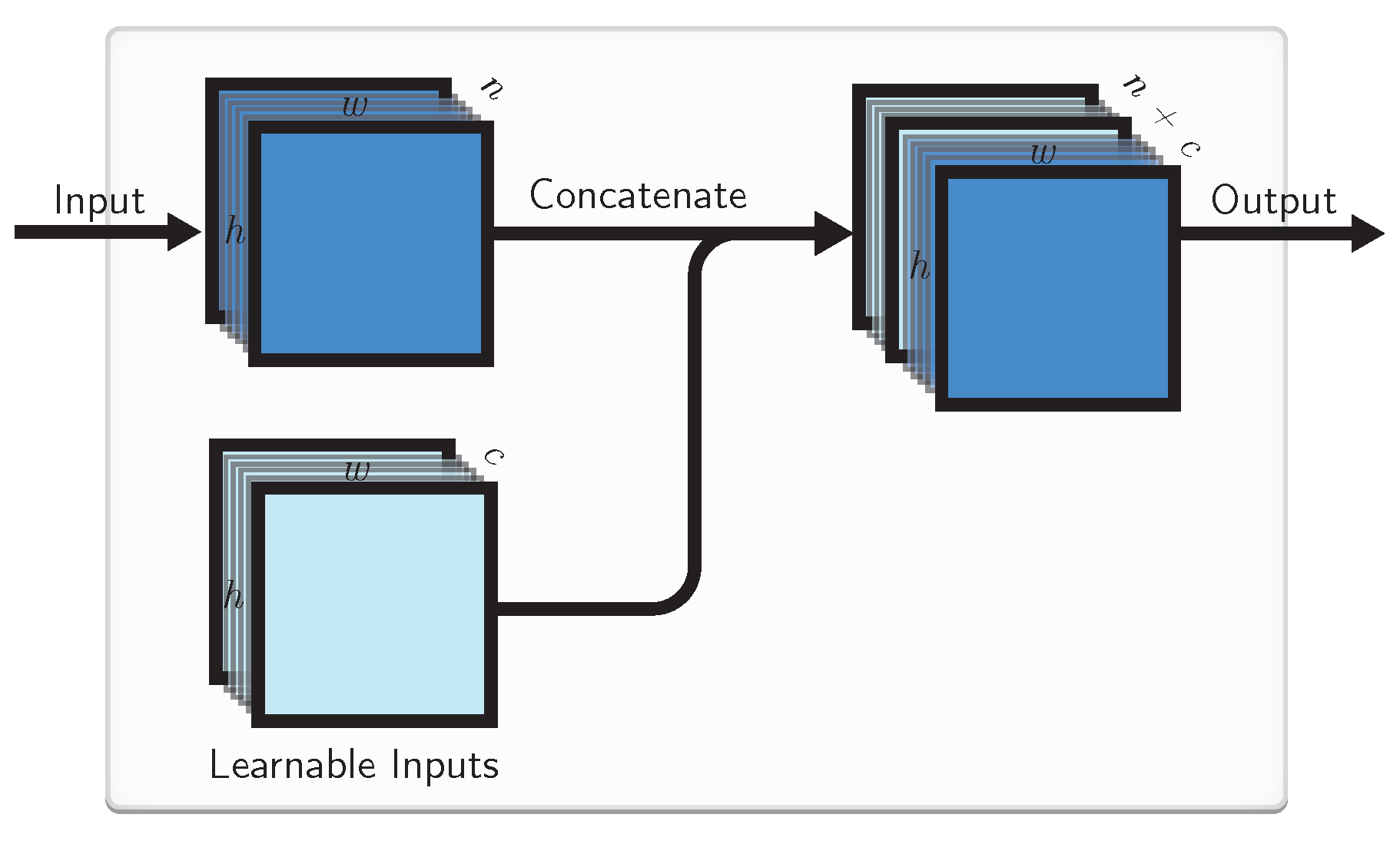
- Learnable local inputs/latent variables,
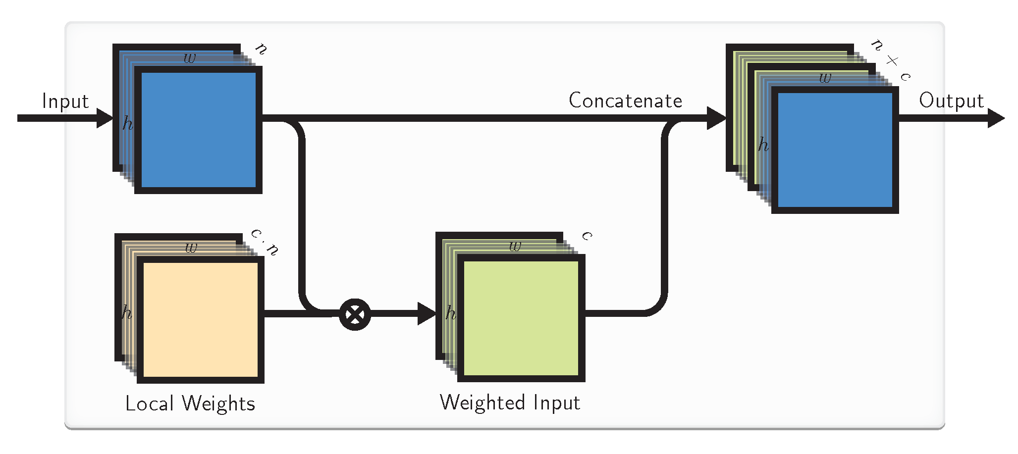
- Learnable local transformations of the inputs in the form of local weights at every input lattice location.
3. Related Work
3.1. Geo-Temporal Prediction
3.2. Previous CNN Localizations
3.3. Deep Input Learning
4. Proposed Methods
4.1. Learnable Inputs
4.2. Local Weights
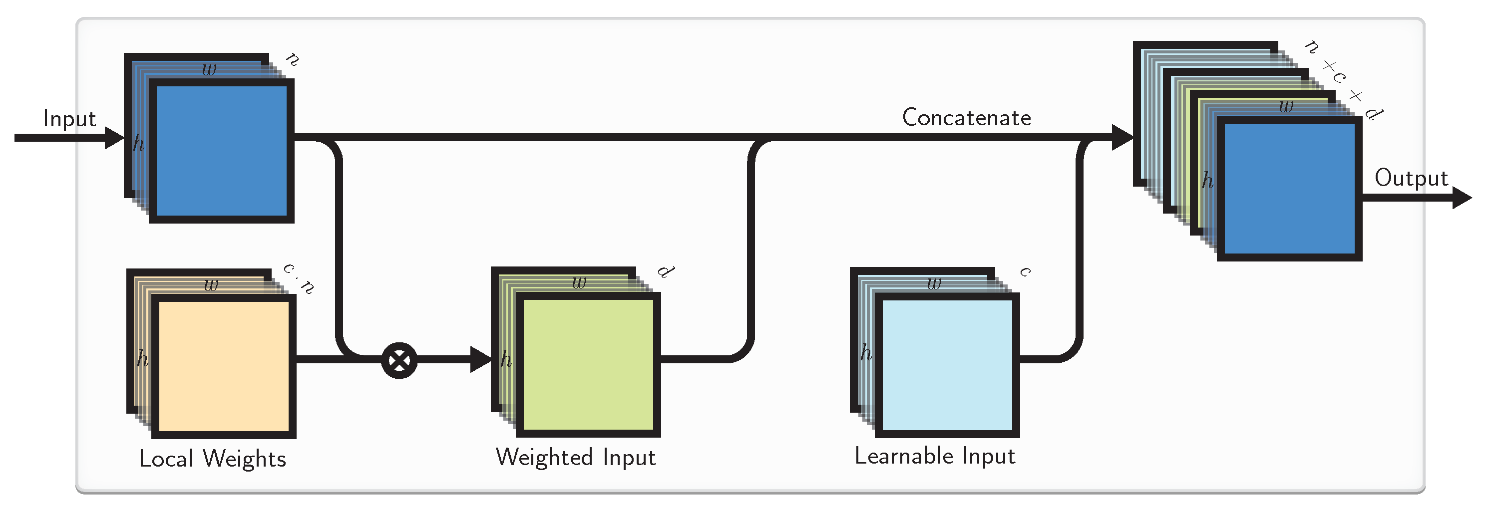
4.3. Combined Approach
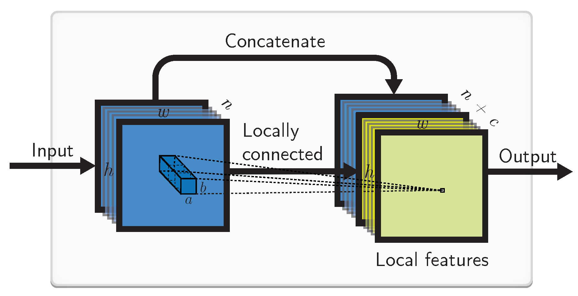
4.4. Implementation by a Locally Connected Layer
5. Baseline and Localized Model Architectures
6. Datasets and Results
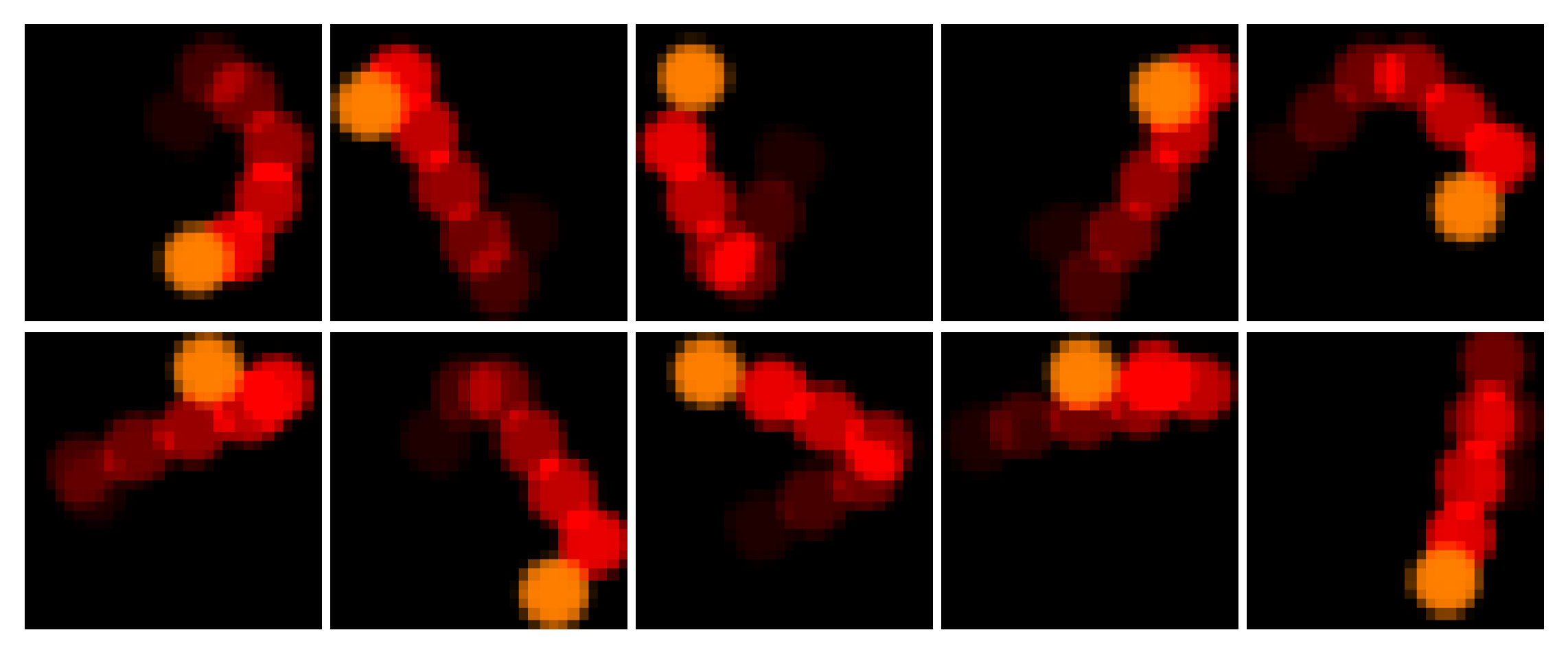
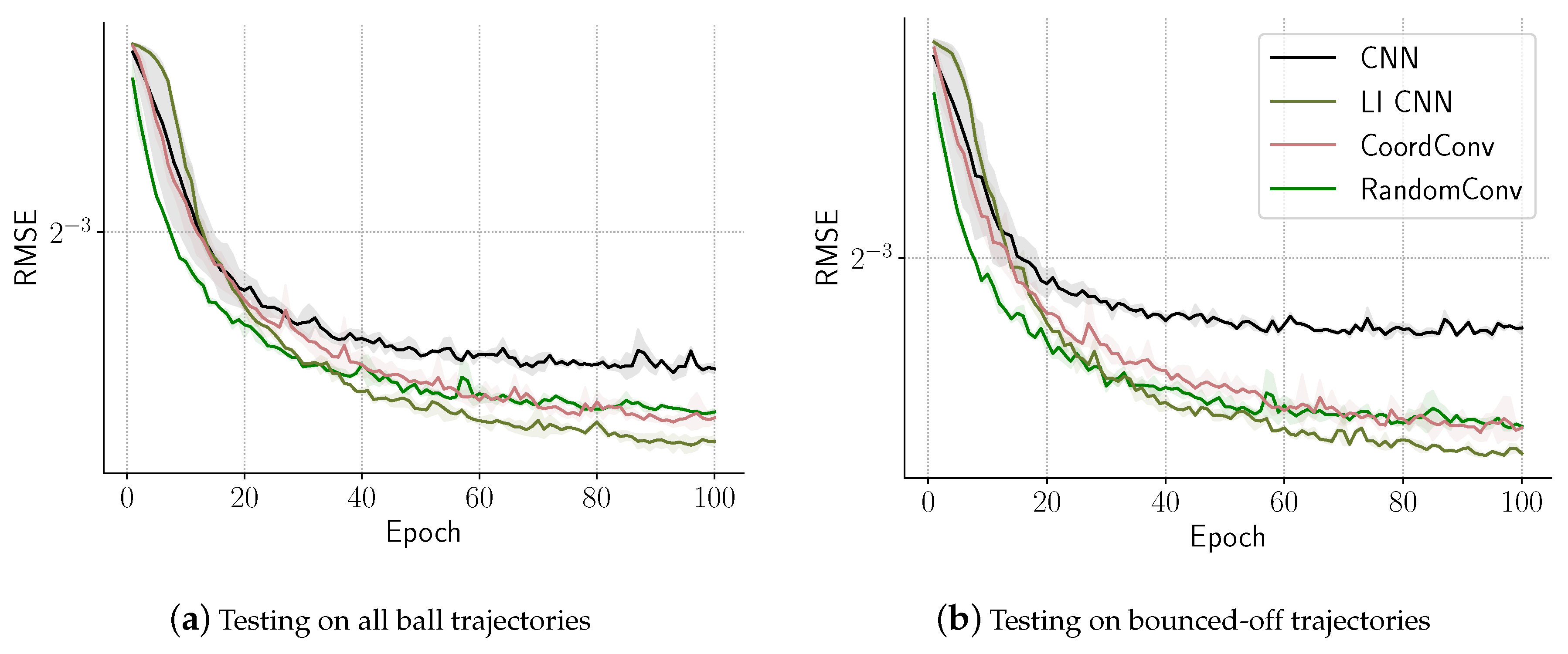
6.1. Proof of Concept: A Bouncing Ball Task
- CNN: a two-layer CNN with filter sizes of and respectively. There are 22 filters in the first layer and 10 filters in the second. This network has 242,043 learnable parameters.
- LI CNN: a similar setup to CNN, except that it has 20 filters in the first layer but two learnable inputs are added to learn location-based features. This network has 237,841 learnable parameters.
- CoordConv: a similar setup to LI CNN, except that it has 21 filters in the first layer and additional x and y coordinate inputs instead of the learnable ones [5]. This network has 247,842 learnable parameters.
- RandomConv: same setup to CoordConv, except that the two inputs were randomly initialized in range. The number of learnable parameters remained the same as in the CoordConv setup.
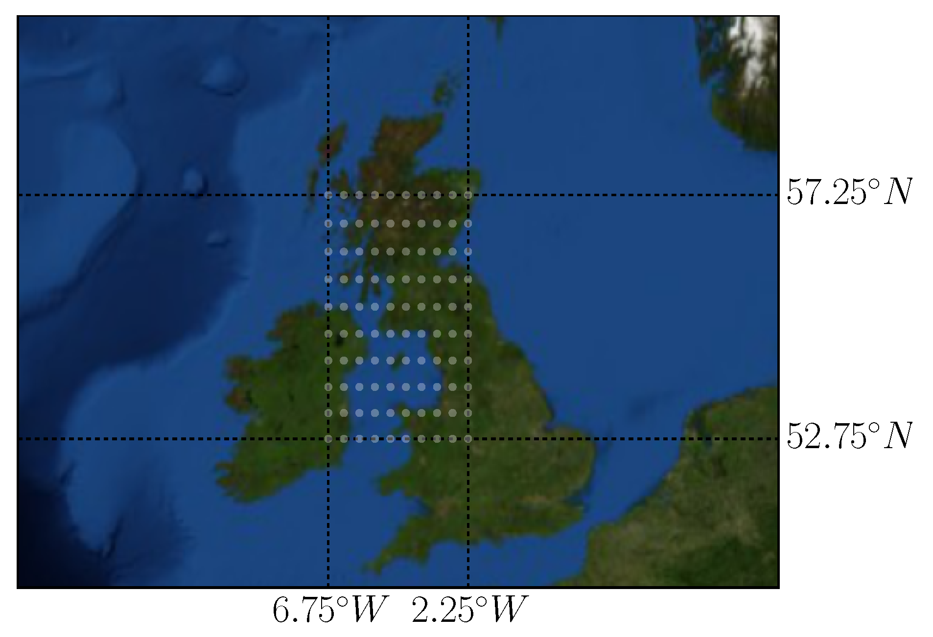
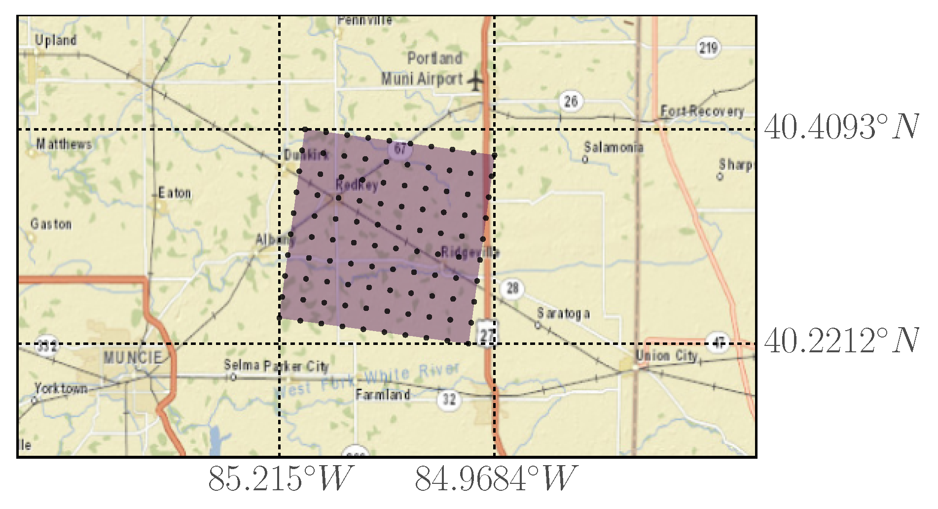
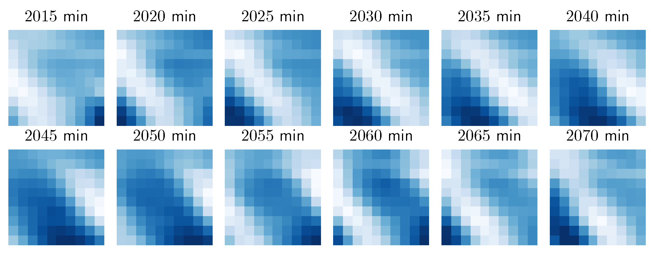
6.2. Case Study: Wind Integration National Dataset
6.3. Case Study: Meteorological Terminal Aviation Routine Dataset
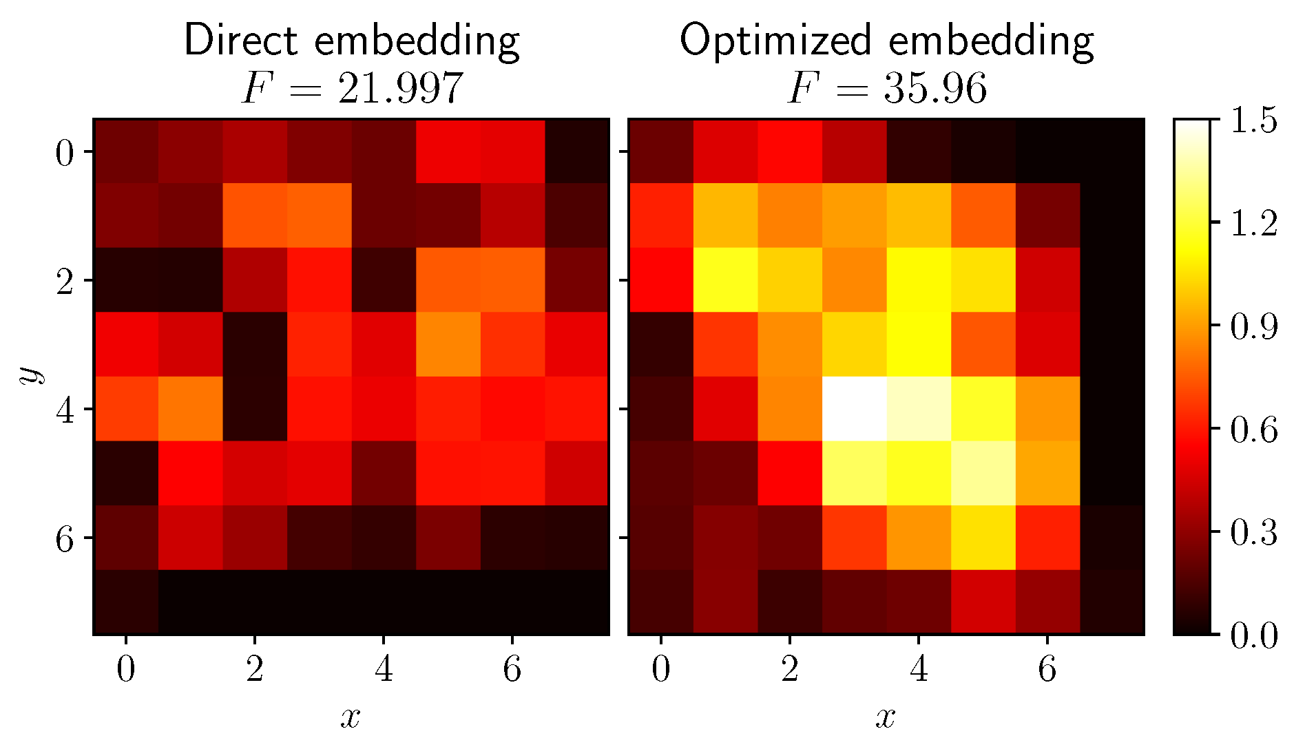
6.3.1. Mutual Information Based Grid Embedding
6.3.2. Results
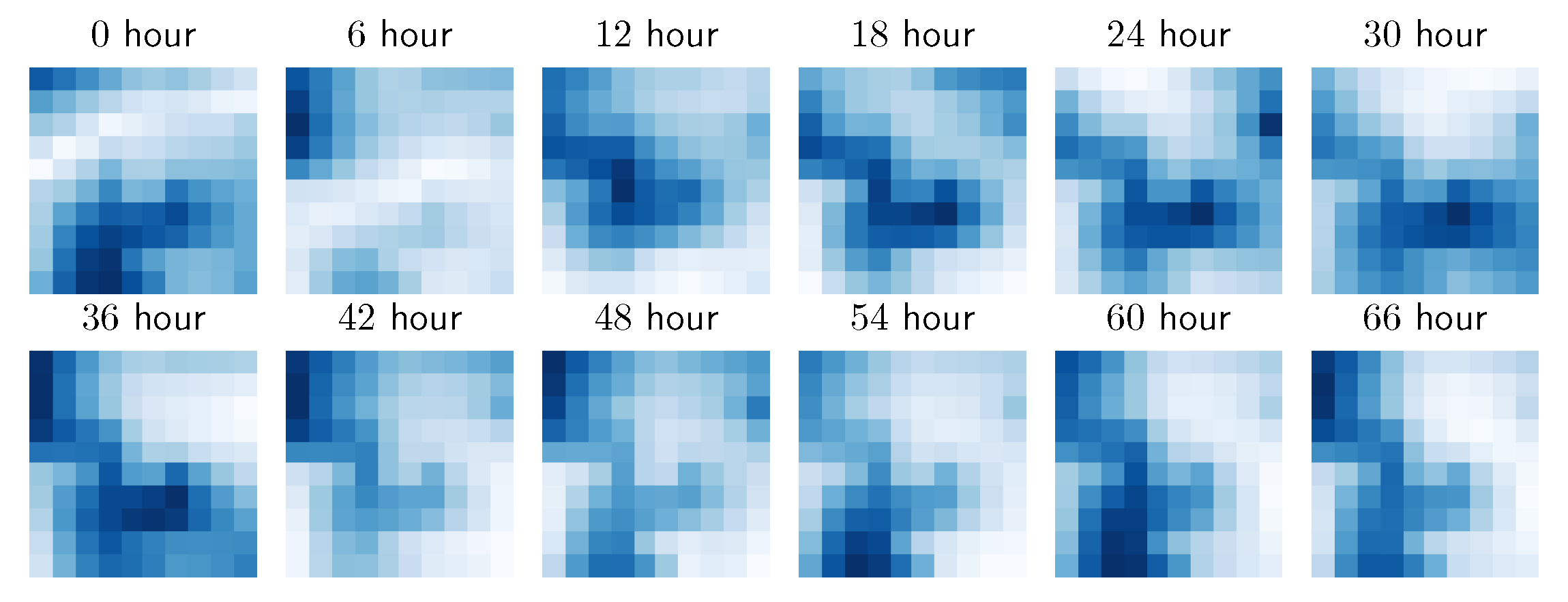
6.4. Case Study: Copernicus Dataset
7. Conclusions and Future Directions
Supplementary Materials
Author Contributions
Funding
Conflicts of Interest
References
- Shi, X.; Yeung, D.Y. Machine Learning for Spatiotemporal Sequence Forecasting: A Survey. arXiv 2018, arXiv:1808.06865. [Google Scholar]
- LeCun, Y.; Bottou, L.; Bengio, Y.; Haffner, P. Gradient-based learning applied to document recognition. Proc. IEEE 1998, 86, 2278–2324. [Google Scholar] [CrossRef] [Green Version]
- LeCun, Y.; Boser, B.; Denker, J.S.; Henderson, D.; Howard, R.E.; Hubbard, W.; Jackel, L.D. Backpropagation Applied to Handwritten Zip Code Recognition. Neural Comput. 1989, 1, 541–551. [Google Scholar] [CrossRef]
- Taigman, Y.; Yang, M.; Ranzato, M.; Wolf, L. DeepFace: Closing the Gap to Human-Level Performance in Face Verification. In Proceedings of the 2014 IEEE Conference on Computer Vision and Pattern Recognition, Columbus, OH, USA, 23–28 June 2014; pp. 1701–1708. [Google Scholar]
- Liu, R.; Lehman, J.; Molino, P.; Such, F.P.; Frank, E.; Sergeev, A.; Yosinski, J. An intriguing failing of convolutional neural networks and the coordconv solution. arXiv 2018, arXiv:1807.03247. [Google Scholar]
- Ackermann, T. Wind energy technology and current status: A review. Renew. Sustain. Energy Rev. 2000, 4, 315–374. [Google Scholar] [CrossRef]
- Shi, X.; Chen, Z.; Wang, H.; Yeung, D.Y.; Wong, W.k.; Woo, W.C. Convolutional LSTM Network: A Machine Learning Approach for Precipitation Nowcasting. In Advances in Neural Information Processing Systems 28; Cortes, C., Lawrence, N.D., Lee, D.D., Sugiyama, M., Garnett, R., Eds.; Curran Associates, Inc.: Red Hook, NY, USA, 2015; pp. 802–810. [Google Scholar]
- Yao, H.; Tang, X.; Wei, H.; Zheng, G.; Li, Z. Revisiting spatial-temporal similarity: A deep learning framework for traffic prediction. In Proceedings of the AAAI Conference on Artificial Intelligence, Honolulu, HI, USA, 27 January–1 February 2019; Volume 33, pp. 5668–5675. [Google Scholar]
- Yao, H.; Wu, F.; Ke, J.; Tang, X.; Jia, Y.; Lu, S.; Gong, P.; Ye, J.; Li, Z. Deep Multi-View Spatial-Temporal Network for Taxi Demand Prediction. In Proceedings of the Thirty-Second AAAI Conference on Artificial Intelligence, New Orleans, LA, USA, 2–7 February 2018. [Google Scholar]
- Yi, X.; Zhang, J.; Wang, Z.; Li, T.; Zheng, Y. Deep Distributed Fusion Network for Air Quality Prediction. In Proceedings of the 24th ACM SIGKDD International Conference on Knowledge Discovery & Data Mining—KDD ’18, London, UK, 19–23 August 2018. [Google Scholar] [CrossRef]
- Karpathy, A.; Toderici, G.; Shetty, S.; Leung, T.; Sukthankar, R.; Li, F.-F. Large-scale video classification with convolutional neural networks. In Proceedings of the IEEE Conference on Computer Vision and Pattern Recognition, Columbus, OH, USA, 23–28 June 2014; pp. 1725–1732. [Google Scholar]
- Ng, J.Y.-H.; Hausknecht, M.; Vijayanarasimhan, S.; Vinyals, O.; Monga, R.; Toderici, G. Beyond short snippets: Deep networks for video classification. In Proceedings of the IEEE Conference on Computer Vision and Pattern Recognition, Boston, MA, USA, 7–12 June 2015; pp. 4694–4702. [Google Scholar]
- Zhu, Q.; Chen, J.; Zhu, L.; Duan, X.; Liu, Y. Wind Speed Prediction with Spatio–Temporal Correlation: A Deep Learning Approach. Energies 2018, 11, 705. [Google Scholar] [CrossRef] [Green Version]
- Hochreiter, S.; Schmidhuber, J. Long Short-Term Memory. Neural Comput. 1997, 9, 1735–1780. [Google Scholar] [CrossRef] [PubMed]
- Zhu, Q.; Chen, J.; Shi, D.; Zhu, L.; Bai, X.; Duan, X.; Liu, Y. Learning Temporal and Spatial Correlations Jointly: A Unified Framework for Wind Speed Prediction. IEEE Trans. Sustain. Energy 2020, 11, 509–523. [Google Scholar] [CrossRef]
- Yu, R.; Liu, Z.; Li, X.; Lu, W.; Ma, D.; Yu, M.; Wang, J.; Li, B. Scene learning: Deep convolutional networks for wind power prediction by embedding turbines into grid space. Appl. Energy 2019, 238, 249–257. [Google Scholar] [CrossRef] [Green Version]
- Huang, G.; Liu, Z.; Van Der Maaten, L.; Weinberger, K.Q. Densely connected convolutional networks. In Proceedings of the IEEE Conference on Computer Vision and Pattern Recognition, Honolulu, HI, USA, 21–26 July 2017; pp. 4700–4708. [Google Scholar]
- Woo, S.; Park, J.; Park, J. Predicting Wind Turbine Power and Load Outputs by Multi-task Convolutional LSTM Model. In Proceedings of the 2018 IEEE Power Energy Society General Meeting (PESGM), Portland, OR, USA, 5–9 August 2018; pp. 1–5. [Google Scholar]
- Chen, Y.; Zhang, S.; Zhang, W.; Peng, J.; Cai, Y. Multifactor spatio-temporal correlation model based on a combination of convolutional neural network and long short-term memory neural network for wind speed forecasting. Energy Convers. Manag. 2019, 185, 783–799. [Google Scholar] [CrossRef]
- Novotny, D.; Albanie, S.; Larlus, D.; Vedaldi, A. Semi-convolutional Operators for Instance Segmentation. In Proceedings of the Computer Vision—ECCV 2018, Munich, Germany, 8–14 September 2018; pp. 89–105. [Google Scholar] [CrossRef] [Green Version]
- Watters, N.; Matthey, L.; Burgess, C.P.; Lerchner, A. Spatial Broadcast Decoder: A Simple Architecture for Learning Disentangled Representations in VAEs. arXiv 2019, arXiv:1901.07017. [Google Scholar]
- Lecun, Y. Generalization and network design strategies. In Connectionism in Perspective; Elsevier: Amsterdam, The Netherlands, 1989. [Google Scholar]
- Abdel-Hamid, O.; Jiang, H. Fast speaker adaptation of hybrid NN/HMM model for speech recognition based on discriminative learning of speaker code. In Proceedings of the 2013 IEEE International Conference on Acoustics, Speech and Signal Processing, Vancouver, BC, Canada, 26–31 May 2013; pp. 7942–7946. [Google Scholar]
- Abdel-Hamid, O.; Jiang, H. Rapid and effective speaker adaptation of convolutional neural network based models for speech recognition. In Proceedings of the Interspeech, Lyon, France, 25–29 August 2013. [Google Scholar]
- Xue, S.; Abdel-Hamid, O.; Jiang, H.; Dai, L.; Liu, Q. Fast Adaptation of Deep Neural Network Based on Discriminant Codes for Speech Recognition. IEEE/ACM Trans. Audio Speech Lang. Process. 2014, 22, 1713–1725. [Google Scholar] [CrossRef]
- Gatys, L.A.; Ecker, A.S.; Bethge, M. A neural algorithm of artistic style. arXiv 2015, arXiv:1508.06576. [Google Scholar] [CrossRef]
- Ioffe, S.; Szegedy, C. Batch normalization: Accelerating deep network training by reducing internal covariate shift. arXiv 2015, arXiv:1502.03167. [Google Scholar]
- Kingma, D.P.; Ba, J. Adam: A Method for Stochastic Optimization. In Proceedings of the 3rd International Conference on Learning Representations, ICLR 2015, San Diego, CA, USA, 7–9 May 2015. [Google Scholar]
- Keras. 2015. Available online: https://keras.io/ (accessed on 19 May 2020).
- Abadi, M.; Agarwal, A.; Barham, P.; Brevdo, E.; Chen, Z.; Citro, C.; Corrado, G.S.; Davis, A.; Dean, J.; Devin, M.; et al. TensorFlow: Large-Scale Machine Learning on Heterogeneous Systems. arXiv 2015, arXiv:1603.04467. [Google Scholar]
- Sutskever, I.; Hinton, G.E.; Taylor, G.W. The Recurrent Temporal Restricted Boltzmann Machine. In Advances in Neural Information Processing Systems 21; Koller, D., Schuurmans, D., Bengio, Y., Bottou, L., Eds.; Curran Associates, Inc.: Red Hook, NY, USA, 2009; pp. 1601–1608. [Google Scholar]
- Draxl, C.; Clifton, A.; Hodge, B.M.; McCaa, J. The Wind Integration National Dataset (WIND) Toolkit. Appl. Energy 2015, 151, 355–366. [Google Scholar] [CrossRef] [Green Version]
- Ghaderi, A.; Sanandaji, B.M.; Ghaderi, F. Deep Forecast: Deep Learning-based Spatio-Temporal Forecasting. arXiv 2017, arXiv:1707.08110. [Google Scholar]
- Shannon, C.E. A Mathematical Theory of Communication. Bell Syst. Tech. J. 1948, 27, 379–423. [Google Scholar] [CrossRef] [Green Version]
- Fortin, F.A.; De Rainville, F.M.; Gardner, M.A.; Parizeau, M.; Gagné, C. DEAP: Evolutionary Algorithms Made Easy. J. Mach. Learn. Res. 2012, 13, 2171–2175. [Google Scholar]


| Model Name | Architecture |
|---|---|
| Persistence PR | . |
| CNN | |
| MultiLayer Perceptron MLP | . |
| LSTM (adopted [13]) | |
| ConvLSTM [7] | |
| PSTN [13] | |
| PDCNN [15] | |
| FC-CNN [16] | |
| E2E [16] | |
| CoordConv [5] | |
| LI CNN | |
| LW CNN | |
| LI + LW CNN | |
| Persistent LI + LW CNN | |
| LI + LW – I CNN | |
| LW222 CNN | |
| LW111 CNN | |
| Model | 5 min | 10 min | 15 min | 20 min | 30 min | 60 min | ||||||
|---|---|---|---|---|---|---|---|---|---|---|---|---|
| Valid | Test | Valid | Test | Valid | Test | Valid | Test | Valid | Test | Valid | Test | |
| PR | 0.3929 | 0.3931 | 0.5848 | 0.5850 | 0.7232 | 0.7231 | 0.8333 | 0.8335 | 1.006 | 1.0079 | 1.3779 | 1.3785 |
| CNN | 0.2851 | 0.3429 | 0.4298 | 0.5009 | 0.5368 | 0.6085 | 0.6198 | 0.6991 | 0.7596 | 0.8685 | 1.0973 | 1.2228 |
| MLP | 0.3181 | 0.3617 | 0.4515 | 0.5038 | 0.5463 | 0.6054 | 0.6216 | 0.6911 | 0.7453 | 0.8460 | 1.0906 | 1.2169 |
| LSTM | 0.3039 | 0.3471 | 0.4366 | 0.5003 | 0.534 | 0.6020 | 0.6138 | 0.6899 | 0.7414 | 0.8444 | 1.0735 | 1.2322 |
| CoordConv [5] | 0.2864 | 0.3447 | 0.4323 | 0.5060 | 0.5402 | 0.6133 | 0.6228 | 0.7026 | 0.7668 | 0.8770 | 1.1007 | 1.2311 |
| ConvLSTM [7] | 0.3014 | 0.3730 | 0.4564 | 0.5438 | 0.5623 | 0.6706 | 0.6438 | 0.7668 | 0.7835 | 0.9259 | 1.137 | 1.3380 |
| PSTN [13] | 0.3373 | 0.3653 | 0.4572 | 0.5120 | 0.5504 | 0.6048 | 0.6245 | 0.6890 | 0.7503 | 0.8364 | 1.0804 | 1.2243 |
| PDCNN [15] | 0.4149 | 0.4358 | 0.5041 | 0.5412 | 0.5785 | 0.6290 | 0.6438 | 0.7064 | 0.7639 | 0.8604 | 1.0872 | 1.2509 |
| E2E [16] | 0.3636 | 0.4250 | 0.4809 | 0.5584 | 0.5714 | 0.6479 | 0.6472 | 0.7371 | 0.7769 | 0.8777 | 1.0973 | 1.2373 |
| FC-CNN [16] | 0.4131 | 0.4669 | 0.5164 | 0.5888 | 0.5861 | 0.6613 | 0.6635 | 0.7582 | 0.7288 | 0.8528 | 1.1074 | 1.2945 |
| LI CNN | 0.2825 | 0.3488 | 0.4289 | 0.5030 | 0.5354 | 0.6143 | 0.621 | 0.7062 | 0.7586 | 0.8656 | 1.0973 | 1.2385 |
| Persistent LI CNN | 0.2812 | 0.3400 | 0.4254 | 0.5014 | 0.5381 | 0.6135 | 0.6204 | 0.7026 | 0.7606 | 0.8616 | 1.0973 | 1.2311 |
| LW CNN | 0.2825 | 0.3438 | 0.4289 | 0.5018 | 0.5354 | 0.6082 | 0.6174 | 0.6980 | 0.7606 | 0.8669 | 1.094 | 1.2263 |
| LW111 CNN | 0.2825 | 0.3419 | 0.428 | 0.5021 | 0.5354 | 0.6098 | 0.6168 | 0.6990 | 0.7576 | 0.8621 | 1.094 | 1.2252 |
| LI + LW CNN | 0.2798 | 0.3378 | 0.4272 | 0.5032 | 0.534 | 0.6072 | 0.6186 | 0.6990 | 0.7591 | 0.8715 | 1.1007 | 1.2359 |
| Persistent LI + LW CNN | 0.2838 | 0.3445 | 0.4306 | 0.5037 | 0.5374 | 0.6091 | 0.6228 | 0.7077 | 0.7606 | 0.8665 | 1.0973 | 1.2303 |
| LI + LW222 CNN | 0.2798 | 0.3375 | 0.4272 | 0.4998 | 0.5326 | 0.6086 | 0.618 | 0.7036 | 0.7591 | 0.8651 | 1.0973 | 1.2350 |
| LI + LW – I CNN | 0.3014 | 0.3550 | 0.4433 | 0.5108 | 0.5483 | 0.6206 | 0.6304 | 0.7150 | 0.7721 | 0.8836 | 1.1107 | 1.2530 |
| Persistent LI PDCNN | 0.3995 | 0.4188 | 0.5019 | 0.5434 | 0.5727 | 0.6300 | 0.6438 | 0.7117 | 0.7576 | 0.8561 | 1.0804 | 1.2372 |
| LI + LW PDCNN | 0.4041 | 0.4305 | 0.4945 | 0.5377 | 0.5714 | 0.6215 | 0.6438 | 0.7042 | 0.7586 | 0.8462 | 1.0804 | 1.2397 |
| LI + LW PSTN | 0.3318 | 0.3594 | 0.4564 | 0.5070 | 0.5456 | 0.6055 | 0.624 | 0.6950 | 0.7498 | 0.8477 | 1.077 | 1.2296 |
| Model | Direct Embedding | Optimized Embedding | ||
|---|---|---|---|---|
| RMSE | MAE | RMSE | MAE | |
| DL-STF (All nodes) * [33] | 1.6200 | 1.1800 | – | – |
| PR | 1.791 ± 0.0000 | 1.238 ± 0.0000 | 1.791 ± 0.0000 | 1.238 ± 0.0000 |
| CNN | 1.527 ± 0.0059 | 1.140 ± 0.0057 | 1.509 ± 0.0084 | 1.119 ± 0.0066 |
| MLP * | 1.578 ± 0.0090 | 1.184 ± 0.0131 | – | – |
| LSTM * | 1.665 ± 0.0150 | 1.232 ± 0.0125 | – | – |
| CoordConv [5] | 1.524 ± 0.0064 | 1.134 ± 0.0066 | 1.519 ± 0.0135 | 1.124 ± 0.0085 |
| ConvLSTM [7] | 1.536 ± 0.0089 | 1.135 ± 0.0066 | 1.503 ± 0.0093 | 1.110 ± 0.0063 |
| PSTN * [13] | 1.724 ± 0.0228 | 1.293 ± 0.0149 | 1.716 ± 0.0113 | 1.271 ± 0.0152 |
| PDCNN * [15] | 1.696 ± 0.0173 | 1.277 ± 0.0151 | 1.696 ± 0.0120 | 1.265 ± 0.0100 |
| E2E [16] | 1.627 ± 0.0087 | 1.224 ± 0.0102 | 1.579 ± 0.0145 | 1.179 ± 0.0132 |
| FC-CNN * [16] | 1.676 ± 0.0210 | 1.255 ± 0.0182 | 1.676 ± 0.0145 | 1.251 ± 0.0076 |
| LI CNN | 1.518 ± 0.0088 | 1.133 ± 0.0074 | 1.505 ± 0.0094 | 1.118 ± 0.0048 |
| LW CNN | 1.516 ± 0.0062 | 1.132 ± 0.0044 | 1.508 ± 0.0091 | 1.120 ± 0.0044 |
| LW111 CNN | 1.511 ± 0.0038 | 1.129 ± 0.0053 | 1.506 ± 0.0055 | 1.122 ± 0.0043 |
| LI + LW CNN | 1.512 ± 0.0079 | 1.131 ± 0.0061 | 1.502 ± 0.0087 | 1.118 ± 0.0079 |
| Persistent LI + LW CNN | 1.507 ± 0.0072 | 1.124 ± 0.0062 | 1.501 ± 0.0077 | 1.111 ± 0.0050 |
| LI + LW222 CNN | 1.508 ± 0.0037 | 1.127 ± 0.0054 | 1.504 ± 0.0071 | 1.117 ± 0.0057 |
| Persistent LI + LW222 CNN | 1.507 ± 0.0044 | 1.126 ± 0.0066 | 1.499 ± 0.0072 | 1.116 ± 0.0057 |
| LI + LW – I CNN | 1.505 ± 0.0066 | 1.126 ± 0.0052 | 1.508 ± 0.0156 | 1.123 ± 0.0121 |
| Persistent LI + LW – I CNN | 1.496 ± 0.0046 | 1.116 ± 0.0047 | 1.492 ± 0.0095 | 1.106 ± 0.0083 |
| LI + LW222 – I CNN | 1.515 ± 0.0080 | 1.136 ± 0.0070 | 1.518 ± 0.0084 | 1.135 ± 0.0084 |
| Persistent LI + LW222 – I CNN | 1.492 ± 0.0058 | 1.113 ± 0.0058 | 1.496 ± 0.0061 | 1.109 ± 0.0082 |
| LI + LW PDCNN * | 1.677 ± 0.0054 | 1.254 ± 0.0086 | 1.675 ± 0.0138 | 1.251 ± 0.0115 |
| LI + LW PSTN * | 1.715 ± 0.0183 | 1.278 ± 0.0177 | 1.712 ± 0.0232 | 1.262 ± 0.0139 |
| Model | 6 h | 12 h | ||
|---|---|---|---|---|
| RMSE | MAE | RMSE | MAE | |
| PR | 1.929 ± 0.0000 | 1.454 ± 0.0000 | 2.688 ± 0.0000 | 2.041 ± 0.0000 |
| MLP | 1.494 ± 0.0013 | 1.117 ± 0.0026 | 2.113 ± 0.0047 | 1.599 ± 0.0041 |
| LSTM | 1.438 ± 0.0007 | 1.068 ± 0.0017 | 2.075 ± 0.0047 | 1.564 ± 0.0041 |
| CNN | 1.491 ± 0.0020 | 1.114 ± 0.0025 | 2.126 ± 0.0015 | 1.609 ± 0.0027 |
| PDCNN [15] | 1.447 ± 0.0023 | 1.081 ± 0.0015 | 2.080 ± 0.0063 | 1.570 ± 0.0071 |
| FC-CNN [16] | 1.458 ± 0.0032 | 1.087 ± 0.0038 | 2.093 ± 0.0055 | 1.576 ± 0.0054 |
| E2E [16] | 1.466 ± 0.0052 | 1.092 ± 0.0046 | 2.103 ± 0.0075 | 1.585 ± 0.0071 |
| CoordConv [5] | 1.496 ± 0.0039 | 1.118 ± 0.0027 | 2.128 ± 0.0020 | 1.608 ± 0.0002 |
| PSTN original [13] | 1.433 ± 0.0080 | 1.064 ± 0.0073 | 2.084 ± 0.0000 | 1.568 ± 0.0000 |
| PSTN [13] bigger | 1.431 ± 0.0023 | 1.063 ± 0.0025 | 2.072 ± 0.0039 | 1.560 ± 0.0004 |
| LI CNN | 1.485 ± 0.0021 | 1.106 ± 0.0019 | 2.124 ± 0.0014 | 1.606 ± 0.0026 |
| LW CNN | 1.486 ± 0.0022 | 1.110 ± 0.0005 | 2.124 ± 0.0021 | 1.607 ± 0.0024 |
| LW111 CNN | 1.485 ± 0.0022 | 1.108 ± 0.0030 | 2.124 ± 0.0025 | 1.607 ± 0.0035 |
| LI + LW CNN | 1.485 ± 0.0026 | 1.108 ± 0.0031 | 2.124 ± 0.0012 | 1.607 ± 0.0004 |
| LI + LW – I CNN | 1.493 ± 0.0043 | 1.114 ± 0.0038 | 2.127 ± 0.0016 | 1.608 ± 0.0029 |
| LI + LW222 CNN | 1.480 ± 0.0033 | 1.105 ± 0.0027 | 2.122 ± 0.0035 | 1.604 ± 0.0048 |
| Persistent LI + LW CNN | 1.485 ± 0.0020 | 1.108 ± 0.0011 | 2.125 ± 0.0016 | 1.607 ± 0.0011 |
| LI + LW PDCNN | 1.442 ± 0.0025 | 1.075 ± 0.0020 | 2.071 ± 0.0062 | 1.563 ± 0.0066 |
| Persistent LI PDCNN CNN | 1.436 ± 0.0055 | 1.071 ± 0.0034 | 2.067 ± 0.0028 | 1.556 ± 0.0022 |
| LI + LW PSTN | 1.420 ± 0.0014 | 1.058 ± 0.0015 | 2.061 ± 0.0012 | 1.553 ± 0.0046 |
© 2020 by the authors. Licensee MDPI, Basel, Switzerland. This article is an open access article distributed under the terms and conditions of the Creative Commons Attribution (CC BY) license (http://creativecommons.org/licenses/by/4.0/).
Share and Cite
Uselis, A.; Lukoševičius, M.; Stasytis, L. Localized Convolutional Neural Networks for Geospatial Wind Forecasting. Energies 2020, 13, 3440. https://doi.org/10.3390/en13133440
Uselis A, Lukoševičius M, Stasytis L. Localized Convolutional Neural Networks for Geospatial Wind Forecasting. Energies. 2020; 13(13):3440. https://doi.org/10.3390/en13133440
Chicago/Turabian StyleUselis, Arnas, Mantas Lukoševičius, and Lukas Stasytis. 2020. "Localized Convolutional Neural Networks for Geospatial Wind Forecasting" Energies 13, no. 13: 3440. https://doi.org/10.3390/en13133440
APA StyleUselis, A., Lukoševičius, M., & Stasytis, L. (2020). Localized Convolutional Neural Networks for Geospatial Wind Forecasting. Energies, 13(13), 3440. https://doi.org/10.3390/en13133440