Article

Condition-Monitoring System for Identification and Representation of the Capability Diagram Limits for Multiple Synchronous Generators in a Hydro Power-Plant

1
HEP-Proizvodnja d.o.o., Hydro Power Plant Vinodol, Sušik 15, 51243 Tribalj, Croatia
2
Faculty of Electrical Engineering and Computing, University of Zagreb, Unska 3, 10000 Zagreb, Croatia
*
Author to whom correspondence should be addressed.
Energies 2020, 13(15), 3800; https://doi.org/10.3390/en13153800
Submission received: 29 June 2020 / Revised: 17 July 2020 / Accepted: 22 July 2020 / Published: 24 July 2020
(This article belongs to the Special Issue Condition Monitoring and Diagnosis of Electrical Machines)

Abstract

:
This paper presents an experience in the design and implementation of the condition-monitoring system for the synchronous generators whose primary purpose is to record data for the identification of the capability limits of the PQ diagram of three generators in hydro power-plant. Paper presents details about the monitoring system, the underlying theory of the identification of the synchronous generator model with a focus on the calculation of the capability limits in the PQ diagram. Furthermore, a computationally efficient method for the representation of capability limits suitable for the implementation within the industrial automation and control system of the power-plant is described in detail. Finally, the capability diagrams for three generators were implemented in the power-plant supervisory control and data acquisition system (SCADA) system.

1. Introduction

The voltage control in the power systems is achieved by reactive power control with units such as capacitor banks, shunt reactors, thyristor switched capacitors (TSC), thyristor switched reactors (TSR) and synchronous generators. Since the synchronous generators are capable of quickly and continuously generating both inductive and capacitive reactive power, synchronous generators with their automatic voltage regulators are traditionally the primary units to control the voltage of the bulk power system. Due to the existence of the static-stability limit at the capacitive region of the synchronous generators, power system operators are often reluctant and restrain from the operation of the synchronous generators in the capacitive region, which restricts their utilization for the voltage control. Therefore, the knowledge on the real limits in the PQ diagram or capability limits of synchronous generators are an essential tool for efficient management of the high voltage networks in power systems. The manufacturers of synchronous generators provide operational limits of the generator, but they are often derived based on the constant synchronous inductances. In the real-world operation, synchronous inductances are not constant, and they are changing with the level of saturation in both direct (d) and quadrature (q) axis of the generator, which varies with the operating point. This means that in practice, there are often uncertainties about the real position of the actual capability limits, which is the reason why the high-voltage operators do not want to use generators in those unknown regions. For the utilization of the generators in those unknown regions, it is required to derive the capability limits in the PQ coordinate system based on the reliable generator model that takes into account their variations due to saturation and the change of the voltage. For the successful utilization in practice, capability diagram limits should also be suitable for the implementation in the power plant and power system control.
There are a lot of models of synchronous machines reported in the literature [1,2,3,4,5,6,7,8,9,10,11,12,13,14,15,16,17,18,19] that are based on the two-axis theory. All of those models were developed for a specific purpose or application and they have their advantages and disadvantages. Dynamical models for synchronous machines can be divided on the models based on constant values in synchronous rotating d-q reference frame, on the models that take into account cross-saturation [2,3,20,21,22,23,24], on the models that were developed in the abc reference frame [9,19]. A special part of the models in the abc reference frame represents the voltage behind reactance type of models [12,13,14,15,16,17,18,19] which are more appropriate for the modelling of the synchronous generators as a part of the power-system.
Some models are purely mathematical (black box models) without the physical background [10,25,26,27,28,29,30,31,32,33,34,35]. Their purpose is to model the input-output relationship in accurate way, but they are often not applicable for other uses and only serves for the purpose that they are initially developed for.
Besides the simulations and analysis of the synchronous machines as a part of electromechanical systems or for synthesis of the field current control [11,29,32,33,36] dynamical models of the synchronous machines are often used for the estimation of the stability of synchronous generators and power system [37,38,39,40].
It is known that the the synchrous reactances are changing with the operating point of the generator which has been reported in literature [6,7,8,22,41,42,43,44,45,46,47,48,49].
A smaller number of papers deal with the steady-state models of the synchronous machines [45,46,47,48,50,51,52,53,54]. An interesting approach is presented in [6,7,8] where the dynamical model of the synchronous generator is identified based on the measurement of the steady-state operating points during on-grid operation. One of the purposes of the steady-state models is the identification of the capability limits in the PQ diagram. Due to the magnetic saturation, cross-magnetisation effect, and variation of the armature voltage, the operational limits will be changing in real-time. The variable capability diagram limits are analysed in [45,46,47,48,55,56,57].
As presented, many synchronous machine models have been reported in the literature. Different models have been developed for various purposes. However, none of the proposed models deal with the problem of determination of the capability limits in the PQ diagram, which is addressed in this paper. Since the capability limits in the PQ diagram are steady-state limits, a steady-state model of the synchronous generator should be used. An accurate steady-state model that incorporates magnetic saturation and the cross-magnetization effect of the synchronous generator is presented in [58] and will be adopted here for the calculation of the capability limits in the PQ diagram. In addition, this paper will provide details on how to calculate capability diagram limits and how to use computationally efficient methods for representation of those limits in real-time and in the industrial environment within the supervisory control and data acquisition system (SCADA) system.
Condition-monitoring systems for synchronous generators are reported in [48,59,60,61]. However, none of the described condition-monitoring systems deals with the logging data for identification of the PQ diagram capability limits for multiple hydro generators in power plants.
This paper presents an experience in the design and implementation of the condition-monitoring system for the synchronous generators whose primary purpose is to collect data for the identification of the capability limits of the PQ diagram of three generators in hydro power-plant. Paper presents details of the monitoring system and underlying theory of the identification of the synchronous generator model with the focus on the calculation of the capability limits. Furthermore, a computationally efficient method for the representation of capability limits suitable for the implementation within the industrial automation and control system of the power-plant is described in detail. Finally, the capability diagrams for three generators were implemented in the power-plant SCADA system.
Paper is organized into six sections. The first section is the introduction, where the motivation for the topic is described and where the literature review is given. The second section provides details on the condition-monitoring system. The third section presents the measured data and identification of the steady-state models for each of the synchronous generators in the power plant. The fourth section deals with the calculation of the capability diagram limits. The fifth section discusses the computationally efficient computation of the capability limits in the PQ diagram capable of the implementation in the power-plant SCADA system. Finally, the conclusion is given in the sixth section. At the end of the paper, there is an appendix with the list of all relevant equipment used for the implementation of this condition-monitoring system.

2. Condition-Monitoring System

2.1. Topology of the Condition-Monitoring System

Figure 1 shows the topology of the condition-monitoring system.
Power-plant consists of three synchronous generator units, each powered with two Pelton turbines (Figure 2). Nominal data of the generators are given in Table 1.
Several sensors and transducers were installed on every generator besides the usual equipment for the current and voltage measurement. Hall probes were installed in the air gaps of the generators, temperature transducers PT1000 were mounted in the end region on the pressure plates, and the proximity sensors were installed on the shaft.
Hall probes should be supplied with a stable current source, which are CS1, CS2, and CS3 shown in Figure 1. Voltage signals from the Hall probes are conditioned with the insulation amplifiers, which are IA1, IA2, and IA3 shown in Figure 1. Additionally, signals from PT1000 transducers are conditioned with the RTD signal conditioner that also provides galvanic insulation, which are TIA1, TIA2, and TIA3 in Figure 1. The current sources, insulation amplifiers, and temperature signal conditioners are all located in the small cabinets near the generators. That is done since the hall sensors and temperature sensors are generating low energy signals which should not be routed with the long cables in the industrial power plant due to noise generation. In addition, to reduce the possibility of noise generation shielded twisted pairs were used for the signal cables.
One of the requirements for the monitoring system was to use the standard industrial equipment as much as possible in order to keep the costs at a reasonable level. Therefore, existing equipment was used for the armature current, and voltage sensing, and only one phase was used for the current and voltage measurement. The current is measured with the current transformers, and voltage is measured with the voltage measurement transformer with divider and insulation amplifier. Current and voltage measurement transformers were already installed in the power-plant in the generator’s synchronization cabinets, and the installation of the new equipment was minimum, which reduced the cost of the system.
Capability diagram cabinet is a central unit of the monitoring system and all the signals were routed to that place. Those signals are conditioned hall probe signals, conditioned temperature signals, rotor proximity signals together with the armature current and voltage. Proximity signals are used with the armature voltage signals for determination of the load angles for each of the generators using a load angle measurement device that is installed at the same location. Signals are acquired using the National Instrument equipment NI c9205 with the chassis NI cDAQ 9181 with the Ethernet communication. The sampling frequency is 20 kHz. Ethernet connection is routed using optical fiber throughout the power-plant from the capability diagram cabinet to the server room where the main computer of the monitoring system is located. Ethernet connections are shown in blue color, while the fiber optics connections are shown in orange color in Figure 1.
Besides acquiring signals and monitoring data using LabView, the computer communicates with the power-plant SCADA system trough the industrial network using PLC S7-300. The computer sends the air-gap flux density data to the SCADA, pressure-plate temperature data and load angle data. It also reads active, reactive, and apparent powers data as well as the values of the field current for each generator. After processing the signals and calculating the capability diagram limits, the computer sends that data to the SCADA were those limits are implemented and shown for every generator in the control room of the power-plant. More details regarding the calculation of the capability limits are given in Section 4.
Figures of the main parts of the condition-monitoring system are shown in Figure 3.
The main computer for condition-monitoring can be remotely accessed via a power plant business network for reviewing and transferring the data. The primary function of the PLC is to access the industrial network and power plant SCADA system and to act as an interface with equipment for the monitoring system. All industrial devices and complete automation of the power plant is controlled trough the industrial network. Since the power-plant is a vital part of the power system, in order to reduce possible cyber attacks, the power plant business network should be strictly separated from the industrial network. PLC provides the barrier between them, and its primary function is exchange measurement data and provide it to the computer and reads the capability limits data from the computer and provide it to the SCADA system. PLC cannot control any other process in the industrial network, which is crucial for ensuring protection against cyber attacks.
The table with all relevant equipment is given in the Appendix A in Table A1.

2.2. Nonstandard Measurements and Features of the Condition-Monitoring System

There are several nonstandard measurements and data acquisition techniques that cannot be seen as a part of the standard power plant measurement equipment, and there are several special features of the condition measurement system.
For example, the flux density in the air gap is measured, an it can be used for diagnostic of the eccentricity of the rotor, short circuits of the turns in the field winding, or for detection some other non-symmetrical magnetic conditions that originate from the rotor side.
The condition-monitoring system acquires and logs all the relevant data for the identification of the synchronous machine model, which is used for the calculation of the capability limits in the PQ diagram. Those data are armature voltage, armature current, phase angle between armature voltage and current, load angle, and the field winding current. All that data are monitored and archived in the database during the regular operation of the generator.
In addition, a transient recorder feature is implemented within the condition-monitoring system. The transient recorder continuously records 20 s of all the acquired waveforms. Proceeding with storing of all the signals is conducted if the transient criteria are met. It this case, the criteria are met if the standard deviation of the RMS of the current during the 20 s window is greater than 0.05 p.u, and if the voltage signal is greater than 0.5 p.u. The storing is then conducted with recorded 5 s before the described criteria are met and 15 s after. The 5 s prebuffer is used to determine the conditions that were in place before the transient occur. This feature is extremely useful for the analysis and determination of the conditions during the sudden trips and fallouts of the generators. During those sudden trips and fallouts of the generators, the power system operation rules prescribe the analysis of the conditions is conducted for determining the causes of the trip and fallouts before the next synchronization. The cost of unplanned stops of the power-plant is very high, and this transient recorder feature is making the analysis fast and efficient, hence reducing the time and expenses of the unplanned power-plant stops.
An example of one transient captured by the transient recorder is shown in Figure 4. Figure 4 shows the synchronisation event.
One of the crucial quantities for identification of the synchronous generator model is the measurement of the load angle, which surely is a nonstandard measured quantity. For load angle measurement, a special micro-controller based device has been developed. The operational principle of the device is shown in Figure 5.
For the determination of the load angle, an arbitrary armature voltage is used. It can be an arbitrary phase or arbitrary line-to-line armature voltage. After scaling to the low-level voltage level, the armature voltage signal is digitalized using a comparator. The comparator compares the armature voltage signal with 0 V and generates a digital signal with a logical high level if the voltage is greater than 0 V and logical zero otherwise. Proximity signal is assumed to be digital, and if that is not true, it can also be digitalized using a comparator. The device measures the time between the rising edge of the proximity signal and the rising edge of the digital signal of the armature voltage after the comparator, which is T 1 in Figure 5.
Additionally, the period of the armature voltage is measured, which is shown in Figure 5 as time T 2 . Time T 1 is proportional to the load angle, but it has an offset that has to be compensated with calibration. Calibration should be done in the no-load condition since the load angle, in that case, is equal to zero degrees. Ideally, the calibration should be conducted before the synchronization of the generator with the grid. Taking all this into account, the load angle can be calculated as
δ = m o d φ p r o x , U φ c a l i b r a t i o n , 360 = m o d T 1 T 2 · 360 T 1 i n n o l o a d T 2 i n n o l o a d · 360 , 360 ,
where φ p r o x , U is the phase angle between rising edges of the proximity signal and digitalized armature voltage after comparator and can be calculated as T 1 T 2 · 360 and φ c a l i b r a t i o n is angle used for calibration which is calculated in the same way only in no load condition T 1 i n n o l o a d T 2 i n n o l o a d · 360 .
The value of the angle φ c a l i b r a t i o n is stored in the micro-controller memory once the calibration is conducted. Modulo function is used in order to correctly calculate the load angle in the case if the proximity angle starts to lagging in respect of the armature signal. Usually, the load angle signal is within the interval of 180 , 180 where negative values are for the motoring mode of the generator. Since the (1) returns the values from 0 , 360 in order to bring down the value of the load angle with the 180 , 180 interval, the value of 360 should be subtracted from the (1) in the case the calculated angle in (1) is greater than 180 .
The described approach for measurement of the load angle is good enough for the measurement of the load angle in steady-state conditions, which is required for the identification of the generator model.
For the redundancy of the system, the load angle is also computed within the Labview. The same described load angle measurement algorithm is implemented in Labview since the armature voltage, and proximity waveform signals are acquired.

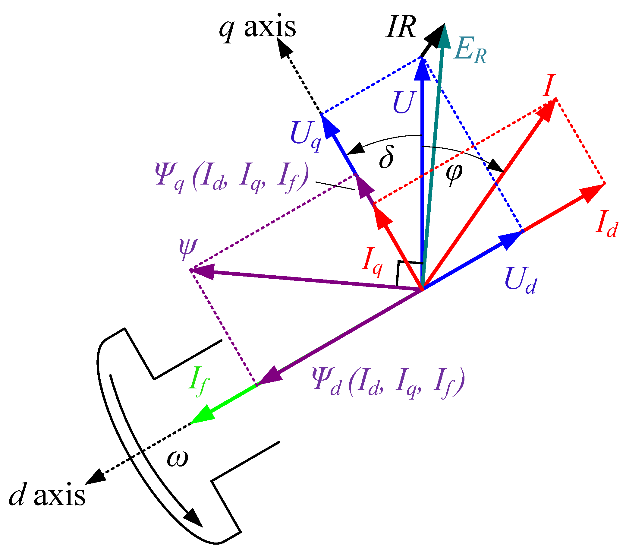
3. Measured Data and Identification of the Current Dependent Flux Linkage Models for the Generators

For the identification of the synchronous machine current-dependent flux linkage model, ideally, there should be as many steady-state operating points as possible spread throughout all the regions of the PQ diagram and acquired during different grid voltage conditions. Realistically, for identification of the model, approximately a hundred operating points recorded for a couple of active and reactive power levels would be sufficient.
The steady-state operating points used for the identification of the current dependent flux linkage model for each of the synchronous generators are shown in Figure 6.
It must be noted that the load angle and field current are also logged together with data shown in Figure 6, which are active and reactive power and armature voltage.
To identify the current dependent flux linkage model for all the generators, firstly, d-q decomposition of the armature current and voltage should be conducted as follows.
U d = U sin δ U q = U cos δ
I d = I sin ( δ φ ) I q = I cos ( δ φ ) ,
where U and I are armature voltage and current, respectively, U d and U q are armature voltage components in d and q axis, I d and I q are armature current components in d and q axis, δ is load angle and φ is power angle i.e., phase angle between armature voltage and current.
Then the flux linkages in the d and q axis ( Ψ d and Ψ q , respectively) can be calculated as
Ψ d = U q + I q R ω U q ω Ψ q = U d + I d R ω U d ω ,
where R is armature resistance per phase and ω is electrical synchronous speed.
Often armature resistance can be neglected, especially for large synchronous generators, however, it will be included in the expressions due to generality.
Afterward, the flux linkages are modeled as polynomial functions of all the currents of the generators, which are I d , I q and field current I f .
Ψ d ( I d , I q , I f ) = d 1 I d + d 2 I q + d 3 I f + d 4 I d 2 + d 5 I q 2 + d 6 I f 2 + d 7 I d I q + d 8 I d I f + d 9 I q I f + d 10 I d 3 + d 11 I q 3 + d 12 I f 3
Ψ q ( I d , I q , I f ) = q 1 I d + q 2 I q + q 3 I f + q 4 I d 2 + q 5 I q 2 + q 6 I f 2 + q 7 I d I q + q 8 I d I f + q 9 I q I f + q 10 I d 3 + q 11 I q 3 + q 12 I f 3
The model is adopted from [58], and it takes into account magnetic saturation and cross-magnetisation effect.
Voltage equations of the armature winding in d-q reference frame can be written as
U d = R I d ω Ψ q ( I d , I q , I f )
U q = R I q + ω Ψ d ( I d , I q , I f ) .
The vector diagram of the synchronous generator based on the current dependent flux linkage model is shown in Figure 7.
In order to identify polynomial current dependent flux linkage functions it is required to determine constants d 1 , d 2 , , d 12 and q 1 , q 2 , , q 12 in the expressions (5) and (6). In this particular case, there are 12 unknown constants for both d and q axis flux linkage functions. This means that it is required to have at least 13 steady-state operating points to identify the model. It is, of course, better if there are more operating points since, in that case, the model can be identified with greater accuracy.
Considering that the measured data is organized in the form of the quadruplets ( I d , i , I q , i , I f , i , Ψ d , i ) for the d axis, and ( I d , i , I q , i , I f , i , Ψ q , i ) for the q axis, identification of the constants d 1 d 12 and q 1 q 12 can be conducted using the least square method. By applying the least square method, it is possible to find constants d 1 d 12 and q 1 q 12 such that the sum of the squares of the error between the model and measurements is minimal. In other words, the least square method ensures that the values of the flux linkage functions obtained from the model represented by (5) and (6) are the best possible fits of the measured data.
In order to proceed with the identification and least square method, goal functions G d and G q are defined as follows
G d = i = 1 N Ψ d , i Ψ d ( I d , i , I q , i , I f , i ) 2 min !
G q = i = 1 N Ψ q , i Ψ q ( I d , i , I q , i , I f , i ) 2 min !
where N is the number of the measured steady-state operating points, Ψ d , i and Ψ q , i represent the flux linkage data values whilst Ψ d ( I d , i , I q , i , I f , i ) and Ψ q ( I d , i , I q , i , I f , i ) is the flux linkage calculated by the model represented with (5) and (6).
Goal functions G d and G q depend on the coefficients of the flux linkage polynomials which are d 1 d 12 and q 1 q 12 . Therefore, to find a minimum of G d and G q it is required to find derivatives of the goal functions G d and G q with respect to the variables that they depend on, which are, in this case, d 1 d 12 and q 1 q 12 and equalize that expressions to zero.
G d d k = 0 , f o r k = 1 12
G q q k = 0 , f o r k = 1 12
The system of the Equations (11) and (12) are linear systems that can easily be solved. Therefore the process of the identification of the synchronous machine model is reduced to solving the linear system. For more details, the reader is directed to [58].
It is advised to conduct the identification of the flux linkage functions and synchronous generator model using p.u. values.
Identified coefficients of current dependent flux linkage functions for each generator are given in Table 2.
Once the flux linkage functions Ψ d ( I d , I q , I f ) and Ψ q ( I d , I q , I f ) are identified, and their coefficients are determined, all other quantities in the generator can be calculated using those functions. For example, all other steady-state operating points can be calculated using flux linkage functions. If we define the steady-state operating point with the three quantities which are active power P, reactive power Q and armature voltage U and if we set the following system of the equations
P = ω Ψ d ( I d , I q , I f ) I q Ψ q ( I d , I q , I f ) I d I d 2 + I q 2 R
Q = ω Ψ d ( I d , I q , I f ) I d Ψ q ( I d , I q , I f ) I q
U = ω Ψ d ( I d , I q , I f ) I q R 2 + ω Ψ q ( I d , I q , I f ) I d R 2
then by simultaneous solving the system (13)–(15) it is possible to find currents I d , I q and I f for that operating point. Since the system (13)–(15) is nonlinear, it can be solved using iterative schemes such as the Newtonian or quasi-Newtonian method. Initial values for solving in the iterative scheme can be calculated using classical theory with constant synchronous reactances X d and X q and vector diagram.

4. Calculation of the Operational Limits in the PQ Diagram

Once the current dependent flux linkage models are identified for every generator, those models can be used for the calculation of the operational limits in the PQ diagram. Three different operational limits will be covered in this paper. Those are the maximum armature current limit, constant field current limit, and steady-state stability limit. Turbine limits are not covered in this paper, but they can be estimated as constant active power limits in the PQ diagram.

4.1. Maximum Armature Current Limit

Since the maximum armature current I m a x is 1 p.u. and since the maximum apparent power in p.u. system S m a x is given as the product of the armature voltage U and maximum armature current I m a x , the maximum apparent power is determined by the p.u. value of the armature voltage U
S m a x = U · I m a x = U · 1 p . u . = U ( values are in p . u . ) .
Therefore, the maximum armature current limit in the PQ coordinate system is the circle with the radius that corresponds to the p.u. value of the armature voltage.

4.2. Constant Field Current Limit

For the calculation of the constant field current limit, it is required to ensure that the field current is fixed to the constant value in all the expressions. Therefore, the following should be applied
I f = c o n s t . = I f , c o n s t .
Since the capability diagram limits are calculated for the constant armature voltage, for an arbitrary value of the I d , the value of the I q can be calculated that satisfies the armature voltage equation.
U d e s = ω Ψ d ( I d , I q , I f , c o n s t ) I q R 2 + ω Ψ q ( I d , I q , I f , c o n s t ) I d R 2
where U d e s is the desired armature voltage value.
Equation (18) can be solved using Newton’s method or any other suitable numerical method. Once Equation (18) is solved, a triplet ( I d , I q , I f , c o n s t ) is obtained which can be substituted into expressions for active and reactive power (13) and (14) in order to obtain pair (P, Q) that can be represented in the PQ diagram. The following procedure should be conducted for various values of the I d in order to obtain the constant field current limit in the PQ diagram. The procedure can also be applied for different values of desired armature voltages U d e s .

4.3. Theoretical Steady-State Stability Limit

Steady-state stability limit of the synchronous generator is due to the fact that there is a maximum value of the torque than can be produced by the generator for a given field current at a constant voltage, regardless of the value of the armature current. That maximum torque corresponds to some value of the active power. In order to determine the steady-state stability limit, different values of maximum active power should be calculated for different values of the field currents. That kind of limit is considered a theoretical steady-state stability limit of the synchronous generator.
To determine a theoretical steady-state stability limit, it is required to fixate the field current and to set I f = I f , c o n s t and find a maximum of the active power while the armature voltage is equal to the prescribed value. Mathematically formulated, it is required to find a conditional maximum of the active power, expressed as (13) with the respect of satisfying the constrain function expressed by armature voltage Equation (15). That conditional maximum can be calculated by utilizing the Lagrange multipliers theory for finding conditional extremes. In order to proceed a Lagrange function L ( I d , I q , λ ) is defined as
L ( I d , I q , λ ) = P + λ U d e s 2 U 2 = ω Ψ d ( I d , I q , I f , c o n s t ) I q Ψ q ( I d , I q , I f , c o n s t ) I d I d 2 + I q 2 R + λ U d e s 2 ω Ψ d ( I d , I q , I f , c o n s t ) I q R 2 + ω Ψ q ( I d , I q , I f , c o n s t ) I d R 2 m a x !
In order to find a maximum of the (19), it is required to solve three equation with three unknowns
L ( I d , I q , λ ) I q = 0 L ( I d , I q , λ ) I d = 0 L ( I d , I q , λ ) λ = 0
Again, the system (20) is nonlinear, and it should be solved using iterative schemes. Once the system is solved, the triplet ( I d , I q , I f , c o n s t ) is obtained as a solution. That solution should be substituted into the expressions for the active and reactive power (13) and (14) in order to obtain PQ pairs that can be represented in the PQ diagram. The described procedure is repeated for the different constant values of the field current I f , c o n s t , which gives the different points on the theoretical steady-state stability limit for a constant armature voltage. The whole procedure can also be used for calculation of the steady-state stability limits for different values of the desired armature voltage of U d e s .

4.4. Practical Steady-State Stability Limit

The practical steady-state stability limit is determined by using 0.1 p.u. of the safety margin compared to the theoretical steady-state stability limit. Therefore, when the maximum power P m a x is calculated, which is the active power that corresponds to the theoretical steady-state stability limit, a new operating point should be calculated, which has lower active power for 0.1 p.u., with the same desired armature voltage and the same value of the field current which is I f , c o n s t . The following system of two equations with two unknowns is obtained
P m a x 0.1 p . u . = ω Ψ d ( I d , I q , I f , c o n s t ) I q Ψ q ( I d , I q , I f , c o n s t ) I d I d 2 + I q 2 R
U d e s = ω Ψ d ( I d , I q , I f , c o n s t ) I q R 2 + ω Ψ q ( I d , I q , I f , c o n s t ) I d R 2
By solving system (21) and (22) the values of the currents I d and I q are obtained and together with the value of the field current I f , c o n s t after their substitution into the expressions (13) and (14) a PQ pair is obtained which can be shown in the capability PQ diagram. By connecting all the calculated PQ points, a practical steady-state stability limit is obtained. The procedure can be used for the calculation of the practical stability limits for the different armature voltages.

5. Computationally Efficient Calculation of the Capability Limits in the PQ Diagram Capable for Implementation in the Power-Plant SCADA System

Clearly, models and calculations presented in the Section 3 and Section 4 are far too complex for being implemented in the standard industrial SCADA system. Furthermore, the calculations for the identification of the generator model and for the calculations of the capability limits are time-consuming, since they are iterative. That is the reason why they are conducted off-line. Therefore, the more suitable and more computation efficient method should be developed for the representation of the capability limits in the on-line real-time environment.
The main idea is to calculate the data set of the operational limits for the different armature voltages and then fit those data to the functions that can be evaluated very fast. In addition, all the evaluations of those functions are conducted at the PC, and only coordinates in the PQ diagram are transferred to the SCADA. Therefore, the SCADA system only shows the connected PQ pairs in the PQ diagram that represents the operational limits.

5.1. Maximum Field Current Limit and Practical Steady-State Stability Limit

The same technique is used for the representation of the maximum field current limit and practical stability limit. Limits are calculated for the different values of the voltage that can be expected during the generator exploitation. Then the reactive power on the limit is fitted to a predefined function with the armature voltage and active power as independent variables Q l i m i t = f ( U , P ) . With the known functions, the values of the active power are predefined as a vector from 0 to maximum active power with approximately ten equidistant values P i . Then, the same number of reactive power values on each limit is calculated using the measured armature voltage.
On the left-hand side of Figure 8, the data are shown for the maximum field current limit.
Precalculated data for the maximum field current and for the practical steady-state stability limit is fit to the same function, which has the following form (23).
Q l i m i t = l 10 U + l 20 U 2 + l 30 U 3 + l 11 U P + l 12 U P 2 + l 13 U P 3 + l 21 U 2 P + l 22 U 2 P 2 + l 23 U 2 P 3
The values of the parameters of the limits functions for maximum field current limit and practical steady-state stability limit for all three generators are given in Table 3.

5.2. Minimum Field Current Limit

A problem with the minimum field current limit is the variation of the maximum active power at the limit with the voltage. Because of that, the active power discretization cannot be predefined as was the case in maximum field and practical steady-state stability limit. That is the reason why the minimum current limits are approximated with the ellipses in the polar coordinate system. Once the minimum field current limits operating points are calculated for various armature voltages, they are fit to the polar ellipse functions. Those ellipse functions have the minor and the major axis, a ( U ) and b ( U ) , respectively, as well as offset in reactive power axis Q 0 ( U ) , which are the functions of the measured armature voltage U.
The ellipses have the following form in the polar coordinate system.
P = a ( U ) sin ( t ) = m 1 U m 2 + m 3 U m 4 s i n ( t )
Q = b ( U ) cos ( t ) + Q 0 ( U ) = m 5 U m 6 + m 7 U m 8 cos ( t ) + m 9 U m 10 + m 11 U m 12
In order to fit data to the ellipses, an optimization is performed with the goal function G e l l i p s e defined as
G e l l i p s e = i = 1 N P i P m o d e l ( Q i , U i ) 2 min !
where P i , Q i and U i are precalculated active power, reactive power and armature voltage data. Function P m o d e l ( Q , U ) is calculated based on (24) and (25) in a following way
P m o d e l ( Q , U ) = a ( U ) 1 Q Q 0 ( U ) 2 b 2 ( U )
The values of the parameters of the limit functions for minimum field current limit for all three generators are given in the Table 4.
The example of limit functions for maximum and minimum field current is shown in Figure 8.

5.3. Implementation of the PQ Diagram with the Real-Time Limits within the Power-Plant SCADA System

The dataflow throughout the condition-monitoring system is shown in Figure 9. Arrows at the Figure 9 designate the information flow.
Once the limits functions are determined using (23)–(25), the values of the actual points in the PQ diagram are calculated at the PC. For that calculation, measured armature voltage is used. Predefined values of active power are used for maximum field current limit and practical steady-state stability limit and predefined values of the parameter t in (24) and (25) are used for the calculation of the minimum current limit. Armature voltage is measured using NI cDAQ equipment for those purposes. PQ pairs for all the limits are sent to the power plant SCADA system from the PC via PLC and industrial network. Within the SCADA system, the PQ diagram is implemented and shown at the control displays in the control room of the power plant. In addition, PC send the load angle, flux density, and temperature measurement data for every generator to the SCADA system for logging and archiving. SCADA system also logs all other relevant data acquired from the generators and the rest of the power plant, which can be used for the analysis and diagnostics of the faulty conditions of the generators.
In addition, data were logged on the PC. Together with the data measured by the monitoring system, which are load angle, armature voltage and current, flux density, and temperature for every generator, additional data obtained from the SCADA system are also logged. The data obtained from the SCADA were active, reactive and apparent power, and field current. All that logged data were used for the identification of the synchronous machine models and for the calculation of the operational limits in the PQ diagram for all the generators in the power-plant. It should be noted that the synchronous machine model and calculation of the operational limits in the PQ diagram and fitting of the functions (23)–(25) are conducted offline. On the other hand, the evaluation of the functions (23)–(25) is done in real-time.
Figure 10 shows the calculated limits of the capability diagram using the limit functions and implemented the PQ diagram in the power plant SCADA.
The proposed methodology takes into account the variation of the operational limits with the armature voltage and with the level of magnetic saturation in the generator. Since the operational limits are obtained from the measured data, they are very accurate, which can be useful for the utilization of the synchronous generators, especially in the underexcited region.

6. Conclusions

The paper presents experiences in the design and details regarding the implementation of the condition-monitoring system for data logging of three generators in the hydropower plant. The primary purpose of the condition-monitoring system is for the identification of the generator models and further determination of the capability diagram limits for each of the generator. This condition-monitoring system uses the standard sensors and transducers which are already installed in the power plant as well as additional custom made equipment for measurement of non-standard quantities. Those non-standard measurement quantities are load angle and air-gap flux density for all three generators.
After the condition-monitoring system has automatically logged the data, the calculations for the identification of the synchronous machine model are conducted, which is followed by the calculation of the capability limits. The theoretical background of those calculations is presented in the paper in detail. In order to implement the PQ diagram with the variable limits in the real-time industrial environment as part of the power-plant SCADA system, a computationally efficient representation of the capability limits has been developed. That computationally efficient representation is based on the limit functions which are fitted to the previously calculated data using identified synchronous machine models. Those limits functions are defined for every limit separately for each generator.
The proposed methodology for data acquisition, monitoring, and logging data, as well as for the identification of the models for the generators and calculation of the capability limits, has been successfully implemented in a hydropower plant with three 35 MVA units and also can be multiplied for more generators in any other power plant. Since the operational limits are obtained from the measured data, they are very accurate, which can be useful for the reliable utilization of the synchronous generators, especially in the underexcited region.

Author Contributions

Initial idea and conceptualisation: M.V. and Z.H.; definition of the condition-monitoring system: M.K., M.V. and Z.H.; theory and methodology of calculation of the operational limits: Z.H., M.V. and B.G.; computational efficient calculation of the operational limits: Z.H., M.K., M.V. and B.G.; implementation of the condition monitoring system and conducting measurements: M.K., B.G. and Z.H.; writing original draft: B.G. and Z.H., editing, writing and final preparation of the paper: M.K. and M.V. All authors have read and agreed to the published version of the manuscript.

Funding

This research received no external funding.

Conflicts of Interest

The authors declare no conflict of interest.

Abbreviations

The following abbreviations are used in this manuscript:
SCADAsupervisory control and data acquisition system
PLCProgrammable logic controller

Appendix A. Used Equipment

Table A1. List of used equipment.
EquipmentDesignation and Description
Existing voltage transformer in power-plant10 kV/100 V, class: 0.5
Existing current transformer in power-plant2000 A/1A, class: 0.5
Installed current transformerDent CT-SRS-005-U, 2.5 A/0.333 V, class 0.2
Voltage divider2 × 22 k Ω
Proximity sensorBalluff BES M18MI-PSC50B-BV10
Temperature sensorPT1000
Hall probeHGT-2010
Supply for the hall probes24 V, 50 mA, custom made
Signal conditioner for PT1000Weidmueller WAS5 PRO RTD 1000
Signal conditioner for current and voltage measurementsWeidmueller WAS4 PRO DC/DC
NI chassisNI cDAQ 9181
NI voltage input moduleNI 9205
Optic converterPlanet, IGT-905A, SFP module
Device for power angle measurementCustom made
PLCSimatic S7-300 CPU 315-2 PN/DP

References

  1. Hamidifar, S.; Kar, N. A Novel Approach to Saturation Characteristics Modeling and Its Impact on Synchronous Machine Transient Stability Analysis. IEEE Trans. Energy Convers. 2012, 27, 139–150. [Google Scholar] [CrossRef]
  2. Levi, E.; Levi, V. Impact of dynamic cross-saturation on accuracy of saturated synchronous machine models. IEEE Trans. Energy Convers. 2000, 15, 224–230. [Google Scholar] [CrossRef]
  3. Mirosevic, M.; Maljkovic, Z.; Miskovic, M. The effect of implementing of dynamic cross saturation on modeling of synchronous generator. In Proceedings of the 2013 Fourth International Conference on Power Engineering, Energy and Electrical Drives (POWERENG), Istanbul, Turkey, 13–17 May 2013; pp. 1477–1481. [Google Scholar] [CrossRef]
  4. Karayaka, H.; Keyhani, A.; Heydt, G.; Agrawal, B.; Selin, D.A. Synchronous generator model identification and parameter estimation from operating data. IEEE Trans. Energy Convers. 2003, 18, 121–126. [Google Scholar] [CrossRef] [Green Version]
  5. Karrari, M.; Malik, O. Identification of Heffron-Phillips model parameters for synchronous generators using online measurements. IEEE Proc. Gener. Transm. Distrib. 2004, 151, 313–320. [Google Scholar] [CrossRef]
  6. Despalatovic, M.; Jadric, M.; Terzic, B. Modeling of Saturated Synchronous Generator Based on Steady-State Operating Data. IEEE Trans. Ind. Appl. 2012, 48, 62–69. [Google Scholar] [CrossRef]
  7. Despalatovic, M.; Jadric, M.; Terzic, B. Modeling of saturated synchronous generator based on steady-state operating data. In Proceedings of the 2010 XIX International Conference on Electrical Machines (ICEM), Rome, Italy, 6–8 September 2010; pp. 1–6. [Google Scholar] [CrossRef]
  8. Jadrić, M.; Despalatović, M.; Terzić, B. Development of synchronous generator saturation model from steady-state operating data. Electr. Power Syst. Res. 2010, 80, 1323–1331. [Google Scholar] [CrossRef]
  9. Marti, J.; Louie, K. A phase-domain synchronous generator model including saturation effects. IEEE Trans. Power Syst. 1997, 12, 222–229. [Google Scholar] [CrossRef]
  10. Garcia-Dominguez, M.; Ruiz-Vega, D. An alternative synchronous machine model for Quasi-Steady-State simulations. In Proceedings of the 40th North American Power Symposium (NAPS ’08), Calgary, AB, Canada, 28–30 September 2008; pp. 1–7. [Google Scholar] [CrossRef]
  11. Racewicz, S.; Riu, D.; Retiere, N.; Chrzan, P. Half-Order Modeling of Saturated Synchronous Machine. IEEE Trans. Ind. Electr. 2014, 61, 5241–5248. [Google Scholar] [CrossRef]
  12. Wang, L.; Jatskevich, J. A Voltage-Behind-Reactance Synchronous Machine Model for the EMTP-Type Solution. IEEE Trans. Power Syst. 2006, 21, 1539–1549. [Google Scholar] [CrossRef]
  13. Huang, Y.; Chapariha, M.; Therrien, F.; Jatskevich, J.; Marti, J. A Constant-Parameter Voltage-Behind-Reactance Synchronous Machine Model Based on Shifted-Frequency Analysis. IEEE Trans. Energy Convers. 2015. [Google Scholar] [CrossRef]
  14. Cramer, A.; Loop, B.; Aliprantis, D. Synchronous Machine Model With Voltage-Behind-Reactance Formulation of Stator and Field Windings. IEEE Trans. Energy Convers. 2012, 27, 391–402. [Google Scholar] [CrossRef]
  15. Karaagac, U.; Mahseredjian, J.; Kocar, I.; Saad, O. An Efficient Voltage-Behind-Reactance Formulation-Based Synchronous Machine Model for Electromagnetic Transients. IEEE Trans. Power Deliv. 2013, 28, 1788–1795. [Google Scholar] [CrossRef]
  16. Liu, S.; Cheng, Y.; Li, L. A voltage-behind-reactance model and validation for six-phase synchronous machines. In Proceedings of the 2014 IEEE Conference and Expo Transportation Electrification Asia-Pacific (ITEC Asia-Pacific), Beijing, China, 31 August–3 September 2014; pp. 1–6. [Google Scholar] [CrossRef]
  17. Wang, L.; Jatskevich, J. Magnetically-Saturable Voltage-Behind-Reactance Synchronous Machine Model for EMTP-Type Solution. IEEE Trans. Power Syst. 2011, 26, 2355–2363. [Google Scholar] [CrossRef]
  18. Aliprantis, D.; Wasynczuk, O.; Rodriguez Valdez, C. A Voltage-Behind-Reactance Synchronous Machine Model with Saturation and Arbitrary Rotor Network Representation. IEEE Trans. Energy Convers. 2008, 23, 499–508. [Google Scholar] [CrossRef]
  19. Pekarek, S.; Walters, E.; Kuhn, B. An efficient and accurate method of representing magnetic saturation in physical-variable models of synchronous machines. IEEE Trans. Energy Convers. 1999, 14, 72–79. [Google Scholar] [CrossRef]
  20. Levi, E. Saturation modelling in d-q axis models of salient pole synchronous machines. IEEE Trans. Energy Convers. 1999, 14, 44–50. [Google Scholar] [CrossRef]
  21. Liang, X.; El-Serafi, A.; Faried, S. Application of the Finite-Element Method for the Determination of the Parameters Representing the Cross-Magnetizing in Saturated Synchronous Machines. IEEE Trans. Energy Convers. 2010, 25, 70–79. [Google Scholar] [CrossRef]
  22. Stumberger, B.; Stumberger, G.; Dolinar, D.; Hamler, A.; Trlep, M. Evaluation of Saturation and Cross-Magnetization Effects in Interior Permanent-Magnet Synchronous Motor. IEEE Trans. Ind. Appl. 2003, 39, 1264–1271. [Google Scholar] [CrossRef]
  23. Bianchi, N.; Bolognani, S. Magnetic Models Of Saturated Interior Permanent Magnet Motors Based on Finite Element Analysis. In Proceedings of the 33rd IAS Annual Meeting 1998 IEEE Industry Applications Conference, St. Louis, MO, USA, 12–15 October 1998; Volume 1, pp. 27–34. [Google Scholar] [CrossRef]
  24. Tahan, S.A.; Kamwa, I. A two-factor saturation model for synchronous machines with multiple rotor circuits. IEEE Trans. Energy Convers. 1995, 10, 609–616. [Google Scholar] [CrossRef]
  25. Pillutla, S.; Keyhani, A. Neural network based saturation model for round rotor synchronous generator. IEEE Trans. Energy Convers. 1999, 14, 1019–1025. [Google Scholar] [CrossRef]
  26. Pillutla, S.; Keyhani, A. Neural network based modeling of round rotor synchronous generator rotor body parameters from operating data. IEEE Trans. Energy Convers. 1999, 14, 321–327. [Google Scholar] [CrossRef]
  27. Abido, M.; Abdel-Magid, Y. On-line identification of synchronous machines using radial basis function neural networks. IEEE Trans. Power Syst. 1997, 12, 1500–1506. [Google Scholar] [CrossRef]
  28. Wu, X.; Fan, Y. Synchronous generator model identification using half-complex wavelet nonlinear ARX network. In Proceedings of the International Conference on Electrical Machines and Systems (ICEMS 2008), Wuhan, China, 17–20 October 2008; pp. 20–25. [Google Scholar]
  29. Wamkeue, R.; Jolette, C.; Mabwe, A.; Kamwa, I. Cross-Identification of Synchronous Generator Parameters From RTDR Test Time-Domain Analytical Responses. IEEE Trans. Energy Convers. 2011, 26, 776–786. [Google Scholar] [CrossRef]
  30. Wamkeue, R.; Baetscher, F.; Kamwa, I. Hybrid-State-Model-Based Time-Domain Identification of Synchronous Machine Parameters From Saturated Load Rejection Test Records. IEEE Trans. Energy Convers. 2008, 23, 68–77. [Google Scholar] [CrossRef]
  31. Fard, R.; Karrari, M.; Malik, O. Synchronous generator model identification using Volterra series. In Proceedings of the Power Engineering Society General Meeting, Denver, CO, USA, 6–10 June 2004; Volume 2, pp. 1344–1349. [Google Scholar] [CrossRef]
  32. Fard, R.; Karrari, M.; Malik, O. Synchronous generator model identification for control application using volterra series. IEEE Trans. Energy Convers. 2005, 20, 852–858. [Google Scholar] [CrossRef]
  33. Vakil, V.; Karrari, M.; Rosehart, W.; Malik, O. Synchronous generator model identification using adaptive pursuit method. IEEE Proc. Gener. Transm. Distrib. 2006, 153, 247–252. [Google Scholar] [CrossRef]
  34. Chaudhry, S.; Ahmed-Zaid, S.; Demerdash, N. An artificial-neural-network method for the identification of saturated turbogenerator parameters based on a coupled finite-element/state-space computational algorithm. IEEE Trans. Energy Convers. 1995, 10, 625–633. [Google Scholar] [CrossRef]
  35. Pillutla, S.; Keyhani, A.; Kamwa, I. Neural network observers for on-line tracking of synchronous generator parameters. IEEE Trans. Energy Convers. 1999, 14, 23–30. [Google Scholar] [CrossRef]
  36. Gong, R.; Huang, Y.; Wei, H.; Meng, X.; Xie, L. Design of PID excitation controllers for synchronous generators based on fuzzy RBF neural network. In Proceedings of the International Conference on Electrical Machines and Systems (ICEMS 2008), Wuhan, China, 17–20 October 2008; pp. 122–127. [Google Scholar]
  37. Guha, S.; Kar, N. Saturation Modeling and Stability Analysis of Synchronous Reluctance Generator. IEEE Trans. Energy Convers. 2008, 23, 814–823. [Google Scholar] [CrossRef]
  38. Babaei, E.; Mozaffari Niapour, S.; Tabarraie, M. Design of a non-linear power system stabiliser using the concept of the feedback linearisation based on the back-stepping technique. IET Gener. Transm. Distrib. 2011, 5, 860–868. [Google Scholar] [CrossRef] [Green Version]
  39. Dineley, J.; Mikhail, S. The dynamic stability of a steam turbine driven synchronous generator under leading power factor load conditions. IEEE Trans. Power Appar. Syst. 1975, 94, 288–298. [Google Scholar] [CrossRef]
  40. Wang, L.; Truong, D.N. Dynamic Stability Improvement of Four Parallel-Operated PMSG-Based Offshore Wind Turbine Generators Fed to a Power System Using a STATCOM. IEEE Trans. Power Deliv. 2013, 28, 111–119. [Google Scholar] [CrossRef]
  41. Sellschopp, F.; Arjona, M. Determination of Synchronous Machine Parameters Using Standstill Frequency Response Tests at Different Excitation Levels. In Proceedings of the IEEE International Electric Machines Drives Conference (IEMDC ’07), Antalya, Turkey, 3–5 May 2007; Volume 2, pp. 1014–1019. [Google Scholar] [CrossRef]
  42. El-Serafi, A.; Kar, N. Methods for determining the q-axis saturation characteristics of salient-pole synchronous machines from the measured d-axis characteristics. IEEE Trans. Energy Convers. 2003, 18, 80–86. [Google Scholar] [CrossRef]
  43. MacDonald, D.; Reece, A.; Turner, P. Turbine-generator steady-state reactances. IEEE Proc. Gener. Transm. Distrib. 1985, 132, 101–108. [Google Scholar] [CrossRef]
  44. Mandić, I.; Tomljenović, V.; Pužar, M. Sinkroni i Asinkroni Električni Strojevi; Polytechnic of Zagreb, Electrical Engineering Department: Zagreb, Croatia, 2012. [Google Scholar]
  45. Ilić, I.; Maljković, Z.; Gašparac, I.; Pavlica, M.; Ilić-Zubović, D.; Jarić, V.; Višković, A.; Belobrajić, R. An Example of Applying Algorithm to Create the Actual PQ Diagram of a Hydrogenerator. Energija 2007, 56, 456–489. [Google Scholar]
  46. Ilić, I.; Maljković, Z.; Gašparac, I.; Pavlica, M.; Ilić-Zubović, D.; Jarić, V.; Višković, A.; Belobrajić, R. Methodology for Determining the Actual PQ Diagram of a Hydrogwenerators. Energija 2007, 56, 144–181. [Google Scholar]
  47. Maljkovic, Z.; Gasparac, I.; Pavlica, M. Large turbogenerator’s synchronous reactance’s load dependence determined by measurements. In Proceedings of the 2014 International Conference on Electrical Machines (ICEM), Berlin, Germany, 2–5 September 2014; pp. 203–207. [Google Scholar] [CrossRef]
  48. Vrazic, M.; Viskovic, A.; Hanic, Z. User PQ Diagram as a Part of a Synchronous Generator Monitoring System. Elektronika ir Elektrotechnika 2014, 20, 33–38. [Google Scholar] [CrossRef]
  49. Escarela-Perez, R.; Niewierowicz, T.; Campero-Littlewood, E. A study of the variation of synchronous machine parameters due to saturation: A numerical approach. Electr. Power Syst. Res. 2004, 72, 1–11. [Google Scholar] [CrossRef]
  50. Sobczyk, T. Inductanceless model of salient-pole synchronous machines. In Proceedings of the International Symposium on Power Electronics, Electrical Drives, Automation and Motion (SPEEDAM 2008), Ischia, Italy, 11–13 June 2008; pp. 620–625. [Google Scholar] [CrossRef]
  51. Hamidifar, S.; Kar, N.C. A state space synchronous machine model with multifunctional characterization of saturation using Levenberg–Marquardt optimization algorithm. Electr. Power Syst. Res. 2013, 102, 33–41. [Google Scholar] [CrossRef]
  52. Calvo, M.; Malik, O. Synchronous Machine steady-State parameter estimation using neural networks. IEEE Trans. Energy Convers. 2004, 19, 237–244. [Google Scholar] [CrossRef]
  53. Fukami, T.; Matsui, Y.; Hayamizu, T.; Shima, K.; Hanaoka, R.; Takata, S. Steady-state analysis of a permanent-magnet-assisted salient-pole synchronous generator. In Proceedings of the 18th International Conference on Electrical Machines (ICEM 2008), Vilamoura, Portugal, 6–9 September 2008; pp. 1–6. [Google Scholar] [CrossRef]
  54. Fukami, T.; Hayamizu, T.; Matsui, Y.; Shima, K.; Hanaoka, R.; Takata, S. Steady-State Analysis of a Permanent-Magnet-Assisted Salient-Pole Synchronous Generator. IEEE Trans. Energy Convers. 2010, 25, 388–393. [Google Scholar] [CrossRef]
  55. Arjona, L.; Macdonald, D. Saturation effects on the steady-state stability limit of turbine-generators. IEEE Trans. Energy Convers. 1999, 14, 133–138. [Google Scholar] [CrossRef]
  56. Gargiulo, G.; Mangoni, V.; Russo, M. Capability charts for combined cycle power plants. IEEE Proc. Gener. Transm. Distrib. 2002, 149, 407–415. [Google Scholar] [CrossRef]
  57. Walker, J. Operating characteristics of salient-pole machines. Proc. IEEE Part II Power Eng. 1953, 100, 13–24. [Google Scholar]
  58. Hanic, Z.; Vrazic, M.; Maljkovic, Z. Steady-state synchronous machine model which incorporates saturation and cross-magnetization effects. In Proceedings of the Fourth International Conference on Power Engineering, Energy and Electrical Drives (POWERENG), Istanbul, Turkey, 13–17 May 2013; pp. 1553–1557. [Google Scholar]
  59. Vražić, M.; Kovačić, M.; Hanić, Z. Design of the monitoring system for a synchronous generators in hydro power plant. In Proceedings of the 2012 International Conference on Renewable Energy Research and Applications (ICRERA), Nagasaki, Japan, 11–14 November 2012; pp. 1–5. [Google Scholar] [CrossRef]
  60. Ehya, H.; Sadeghi, I.; Faiz, J. Online condition monitoring of large synchronous generator under eccentricity fault. In Proceedings of the 2017 12th IEEE Conference on Industrial Electronics and Applications (ICIEA), Siem Reap, Cambodia, 18–20 June 2017; pp. 19–24. [Google Scholar] [CrossRef]
  61. Colak, I.; Garip, I.; Sagiroglu, S.; Bayhan, S. Remote monitoring of the load characteristics of synchronous generators. In Proceedings of the 2011 International Conference on Power Engineering, Energy and Electrical Drives, Malaga, Spain, 11–13 May 2011; pp. 1–4. [Google Scholar] [CrossRef]
Figure 1. Topology of the condition-monitoring system for three generators in a hydro power-plant.
Energies 13 03800 g001
Figure 2. A view at the hydro power-plant turbine room.
Energies 13 03800 g002
Figure 3. Equipment installed in capability diagram cabinet (left) and server room (right).
Energies 13 03800 g003
Figure 4. An example of transient captured by the transient recorder feature of the condition-monitoring system. The recorded transient represents the synchronisation event. The right-hand side figure is a detailed view of the recorded transient which is shown on the left-hand side.
Energies 13 03800 g004
Figure 5. Principle of measurement of the load angle using rotor proximity and armature voltage signal.
Energies 13 03800 g005
Figure 6. Steady-state operating points logged by condition-monitoring system for identification of the synchronous machine models for all the generators.
Energies 13 03800 g006
Figure 7. Vector diagram of the synchronous generator based on the flux linkage model.
Energies 13 03800 g007
Figure 8. The representation of precalculated data and fitted limit functions. An example of maximum field current limit function (left) and minimum field current limit function (right).
Energies 13 03800 g008
Figure 9. Dataflow throughout the condition-monitoring system.
Energies 13 03800 g009
Figure 10. Limits in the PQ diagram calculated using limit functions for three different voltages (left) which are implemented in the power-plant supervisory control and data acquisition system (SCADA) system (right).
Energies 13 03800 g010
Table 1. Nominal data of the of generators.
QuantityValueUnit
Apparent power35MVA
Armature voltage10,500V
Armature current1925A
Frequency50Hz
Rotor speed500rpm
Power factor0.9
Number of phases3
Field current643A
Table 2. Identified coefficients of current dependent flux linkage functions (5) and (6) for all three generators.
G1G2G3 G1G2G3
d 1 2.0062.0711.707 q 1 -0.1570.0780.388
d 2 −0.0110.1040.067 q 2 0.8870.9270.789
d 3 1.8501.7911.581 q 3 −0.0160.1320.472
d 4 −1.062−1.156−0.666 q 4 0.192−0.133−0.661
d 5 −0.421−0.423−0.250 q 5 0.033−0.019−0.369
d 6 −0.900−0.836−0.615 q 6 0.029−0.100−0.526
d 7 0.115−0.089−0.060 q 7 0.004−0.1040.212
d 8 −1.769−1.774−1.139 q 8 0.218−0.177−1.021
d 9 0.036−0.075−0.040 q 9 −0.136−0.1990.002
d 10 0.1390.0990.055 q 10 −0.047−0.0040.220
d 11 0.2570.2250.111 q 11 −0.059−0.0660.221
d 12 0.0600.0480.034 q 12 0.0030.0100.059
Table 3. Limit function parameters for maximum field current and practical steady-state stability limit for all generators.
Maximum Field Current LimitPractical Steady-State Stability Limit
G1G2G3G1G2G3
l 10 −2.1342.628−1.3160.03741−0.8958−1.484
l 20 4.731−7.0765.875−0.2657−2.1532.478
l 30 −1.8394.730−3.894−0.6721−0.07416−1.909
l 11 0.8528−1.5550.35664.1540.5673.632
l 12 −2.704−0.665−0.4793−6.092−3.294−4.300
l 13 0.43549.1444−0.34893.1112.9001.165
l 21 −7.7422.130−0.3111−3.462.107−3.053
l 22 2.4500.090480.18485.7920.8663.987
l 23 −0.4941−0.79890.3871−3.098−1.788−1.045
Table 4. Parameters of the minimum field current limit function for every generator.
G1G2G3
m 1 −1.691120.8262−0.37627
m 2 4.41542.57688.9683
m 3 2.0611−20.52710.6251
m 4 3.74422.65963.5168
m 5 −0.279026.15220.004537
m 6 1.05816.42810.1156
m 7 0.79029−5.73610.31297
m 8 2.92987.04482.1688
m 9 24.1127−3.1951−0.54913
m 10 4.56454.92984.7285
m 11 −25.23622.1303−0.45285
m 12 4.51566.7241.1757

