Abstract
The thermodynamic model is a valuable simulation tool for developing combustion engines. The most widely applied thermodynamic models of spark-ignition engines are the single-zone model and the two-zone model. Compared to the single-zone model, the two-zone model offers more detailed in-cylinder thermodynamic conditions, but its governing equations are numerically stiffer, therefore it is restricted when applied in computationally intensive scenarios. To reduce the two-zone model’s stiffness, this paper isolates an idealized thermodynamic process in the unburned zone and describes this idealized thermodynamic process by an algebraic equation. Assisted with this idealized thermodynamic process, this paper builds a novel two-zone model for spark-ignition engines, whose governing equations are simplified to a set of two ordinary differential equations accompanied by a set of three algebraic equations. Benchmarked against the single-zone model and conventional two-zone model, the novel two-zone model is formed and validated by experimental results, and its stiffness is quantitatively evaluated by linearizing its governing equations at simulation steps. The results show that the novel two-zone model inherits the conventional two-zone model’s ability to estimate both zones’ state variables highly accurately while its simplified structure reduces its stiffness down to the level of the single-zone model, accelerating the computation speed.
1. Introduction
The increasingly stringent regulations on the vehicle emission limits and customer demands for high fuel economy have pushed automotive manufacturers to introduce innovative devices (e.g., variable-geometry turbocharger [1], low- and high-pressure exhaust gas recirculation systems [2]) and sensors (e.g., piezoelectric in-cylinder pressure sensor [3,4]). The innovative technologies make combustion engines more flexible and efficient. However, these innovative technologies really work effectively only under the proper design of the control system and its related management strategies [5].
In order to save development time and costs [6] and to acquire indicating information about the combustion process [7], thermodynamic models have been introduced to assist developing engine control system [8], especially in scenarios where crank-angle resolved outputs are required, e.g., hardware-in-loop (HiL) system simulation, which is required to satisfy strict time constraints with limited computing resources [9]. The concept “zone” is the elementary control volume in the thermodynamic model and can be regarded as the basic structure. In each zone, the first law of thermodynamics and the ideal gas law are applied to govern the state variables [10]. According to the zone number in the combustion chamber, the thermodynamic model can be classified into two main categories [11]: the single-zone model, whose combustion chamber is treated as one zone. And the multi-zone model, whose combustion chamber is divided into several zones.
The single-zone model, the simplest type of thermodynamic models [12], can provide the crank-angle resolved in-cylinder pressure, and requires short CPU time, and has been successfully applied to investigate combustion engine’s behaviors in the real-time environment [13]. Maroteaux et al. developed a single-zone model of a diesel engine for the HiL simulation and modeled the ignition delay time through an Arrhenius correlation and an algebraic simple correlation, and compared their performance [14]. Gambarotta et al. updated a combustion engine module in their in-house Simulink library, which is used in HiL applications, from a mean value model to a single-zone model, and validated the single-zone model of a spark-ignition engine under both steady and transient conditions [15]. Corti et al. packaged the single-zone model into a vehicle longitudinal dynamic simulator and evaluated its ability to reproduce all the signals used as inputs to the control unit based on a motor scooter equipped with a single-cylinder engine and a continuously variable transmission system [16].
The emission estimations are also expected outputs from thermodynamic models [17]. The common approach is to couple the thermodynamic model with a chemical kinetic sub-model [18]: The thermodynamic model is responsible for providing the thermodynamic boundary conditions; and according to these thermodynamic boundary conditions, the chemical kinetic sub-model estimates the emission based on the chemical mechanism. However, the single-zone models are mainly incapable to estimate emissions, especially when the emission formation closely associates with the temperature, because the single-zone models only give an average temperature of the bulk gas [19]. These shortcomings of the single-zone model can be overcome by adopting the multi-zone model, and the most common multi-zone model considers the two zones. Even though more zones adopted in the model may promote the accurate emission estimations, more zones raise computing costs, and at the same time, numerous investigations have shown that the two-zone model is accurate enough to estimate emissions. Provataris et al. developed a two-zone model to estimate the nitrogen oxide (NOx) emissions based on the extended Zeldovich mechanism from two automotive direct-injection diesel engines: a heavy- (truck) and a light-duty (passenger car) engine. Their results show the average absolute percentage error of simulated NOx is respectively 18% and 20% for the truck and car engine [20]. Chindaprasert et al. coupled a two-zone model with CHEMKIN software to predict the carbon monoxide (CO) emissions from a gasoline direct injection engine. Compared to the measured CO emissions, the errors of predicted results under medium and high loads are about −29% while the errors under low load are about −16% [21].
From a mathematical view, the governing equations of a thermodynamic model are a set of ordinary differential equations (ODEs) [22], whose independent variable is the time or the crank angle. Compared to the single-zone model, the two-zone model is much stiffer, resulting in challenges to solve the two-zone model in real-time scenarios. According to the research of Maroteaux et al. on the HiL simulation [14], a quad-core real-time processor computer of three GHz was used, allowing the real-time engine speed of up to 4750 rpm with the resolution of one crank angle degree (CAD). This maximum real-time engine speed covers neither most of the automotive gasoline engines nor some of the high-speed automotive diesel engines. Moreover, the sound solution of the two-zone model is sometimes obtained at a step shorter than one CAD, so it means the maximum real-time engine speed must be further restrained. Therefore, to fulfill the requirement of real-time calculation, the hardware would be upgraded, or the stiffness of the two-zone model should be reduced.
The main objective of this paper is to reduce the model stiffness of the two-zone model to accelerate the computation speed by developing a new modeling algorithm, while low losses of the model features and accuracy are expected when the new modeling algorithm is applied. The idea of this paper is triggered by a new group of thermodynamic models [23], which calculate the thermodynamic states of unburned zone and burned zone based on algebraic equations (AEs) instead of ODEs. This paper calls such models single-to-two-zone models, because these models firstly use the single-zone model, i.e., a set of ODEs, to calculate the cylinder pressure and average temperature, then rearrange the cylinder contents into two-zones and calculate the unburned zone’s and burned zone’s volume and temperature by a set of AEs according to the cylinder pressure and average temperature. Obviously, the mathematical structures of these single-to-two-zone models are similarly complex as the single-zone models. As a result, the computation costs of the single-to-two-zone model are significantly reduced. The single-to-two-zone models explore a new path to accelerating computation from the algorithm. However, such single-to-two-zone models are essentially additives to classic single-zone models. Therefore, some well-developed sub-models for the conventional two-zone model, e.g., flame model, cannot be directly reused by such single-to-two-zone models. This shortage significantly curbs the application of the single-to-two-zone model as a replacement of the conventional two-zone model.
In order to maintain the physical features of the conventional two-zone model, this paper directly algebraizes the differential-form governing equations in the unburned zone of a two-zone model instead of adding AEs on the set of the single-zone model’s differential-form governing equations by the following approach: This paper isolates a thermodynamic process by a pseudo boundary in the unburned zone, and proposes two simplifications to idealize this thermodynamic process as a quasi-isentropic process, then accordingly derives the governing equation of this idealized thermodynamic process by integrating the reduced energy conservation equation of the unburned zone. As a result, the state variables in the unburned can be governed by AEs instead of ODEs. Obviously, the proposed simplifications will change behaviors of the energy conservation equation in the unburned zone. This paper also defines relative errors to analyze these influences from the proposed simplifications.
Based on this idealized thermodynamic process, this paper builds a novel two-zone model for spark-ignition engines, whose governing equations are simplified as a set of two ODEs accompanied by a set of three AEs. The set of ODEs only includes the burned zone’s differential-form energy conservation equation and ideal gas equation of state, and numerically solves the in-cylinder pressure and burned zone’s temperature; The set of AEs includes the volumetric continuity equation and the unburned zone’s algebraic-form the governing equations of quasi-isentropic process and ideal gas equation of state and analytically solves the burned zone’s volume, unburned zone’s volume and temperature.
Benchmarked against the single-zone model and the conventional two-zone model, the novel two-zone model is formed and validated by the experimental data under various working cases, and its stiffness is evaluated by linearizing its governing equations at simulation steps.
2. Description of Model
This section introduces a quasi-isentropic process, and accordingly builds a novel two-zone model. The single-zone model and the conventional two-zone model are selected as the benchmark models of the novel two-zone model. As the single-zone model and the conventional two-zone model have been well established, their governing equations are only briefly introduced in the current section, and further details can be seen in the relevant literature, e.g., reference [24]. The single-zone model, conventional two-zone model, and novel two-zone model use the same sub-models, i.e., engine kinematics, burned mass fraction (using Wiebe function), heat transfer (using Woschni correlation), gas chemical composition and thermodynamic property. These sub-models are described in Appendix A.
The presented thermodynamic models share some common assumptions listed as follows:
- Only the combustion process and the expansion process in the closed cycle of a spark-ignition engine in the steady-state operating conditions are considered in this study.
- The fuel is completely vaporized and well mixed with the incoming air before the models are applied [24].
- Two types of gas models, i.e., unburned gas and burned gas, are adopted in the thermodynamic models. The unburned gas is a mixture of fuel and air, therefore its composition keeps constant in this study. The burned gas is a mixture of combustion products, and its composition varies due to the chemical equilibrium (at the temperature of the zone and the uniform cylinder pressure) [25]. Both unburned gas and burned gas are regarded as the ideal gas, and their composition and thermodynamic properties are spatially uniform in each zone [24].
- The pressure is spatially uniform in the whole combustion chamber, while the temperature is spatially uniform in each zone [24].
- The cylinder wall temperature is assumed to be uniform and keeps constant during the simulation [26].
- All crevice effects are ignored, and the blow-by is assumed to be zero [26]. As a result, the trapped mass of gas in the cylinder is treated as constant during the simulation.
A thermodynamic system in equilibrium can be fully identified by two independent state variables and another state variable for the system size. In this paper, pressure, volume, and temperature are selected as the state variables, i.e., state variables especially refer to these three types of variables in this paper. As the dependent variables in thermodynamic models are usually expected to be crank-angle resolved, the crank angle is selected as the independent variable in this paper, therefore the derivative of a variable is by default with respect to crank angle, namely .
2.1. Formation of Benchmark Models
2.1.1. Formation of a Single-Zone Model
Figure 1 illustrates the schematic of a single-zone thermodynamic model. For a single-zone model, only one zone exists in the combustion chamber.
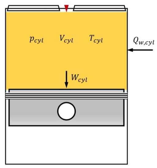
Figure 1.
Schematic of a single-zone thermodynamic model.
The set of the governing equations of the single-zone model consists of 2 equations [24]:
- The differential-form ideal gas law of state in the combustion chamber.
- The energy conservation equation in the combustion chamber.where is the cylinder pressure; is the cylinder volume; is the cylinder temperature; is the trapped mass of gas in cylinder; is the cylinder gas constant; is the specific internal energy of the combustion chamber; is the heat transfer from the cylinder wall to the combustion chamber; is the heat released from the combustion, and its derivative is calculated from lower heating value of the fuel , air-fuel ratio , trapped mass of gas in cylinder and burned mass rate by:
The set of the governing equations of the single-zone model can be written in a matrix-form linearly implicit ODE as:
where is the vector of dependent state variables and in the single-zone model; is the coefficient matrix; is the coefficient vector, i.e.,
2.1.2. Formation of Conventional Two-Zone Model
In a two-zone model, as shown in Figure 2, an infinitesimally thin flame divides the combustion chamber into a burned zone (subscript “b”) and an unburned zone (subscript “u”). The unburned zone is filled with unburned gas, and the burned zone is filled with burned gas.
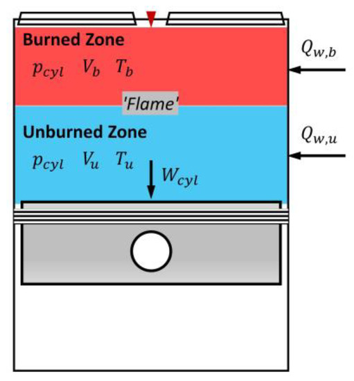
Figure 2.
Schematic of a conventional two-zone thermodynamic model.
The set of the governing equations of the conventional two-zone model consists of 5 equations [24]:
- The differential-form volumetric continuity.
- The differential-form ideal gas law of state in the unburned zone.
- The energy conservation equation in the unburned zone.
- The differential-form ideal gas law of state in the burned zone
- The energy conservation equation in the burned zone.where is the specific enthalpy of the unburned zone; is the specific internal energy of the burned zone; is the heat transfer from the cylinder wall to the unburned zone, is the heat transfer from the cylinder wall to the burned zone.
The gas mass of burned zone and unburned zone are respectively calculated from the total gas mass trapped in cylinder and the burned mass fraction by Equations (13) and (14), and their derivatives, and , are therefore calculated by Equation (15).
The set of the governing equations of the conventional two-zone model can be written in a matrix-form implicit ODE as:
where is the vector of dependent state variables , , , , and in the conventional two-zone model; is the coefficient matrix; is the coefficient vector, i.e.,
2.2. Quasi-Isentropic Process
Figure 3 shows a characteristic thermodynamic process of a two-zone model from a reference condition (subscript ‘r’) before the ignition to a characteristic condition (subscript ‘c’) after the ignition. The ‘reference condition’ can be chosen between the intake-valve-closure and the ignition, and the state variables in the reference condition are required known in advance, e.g., from the boundary condition, or from the last calculation step; The characteristic condition can be arbitrarily chosen after the ignition and before the valve-open, i.e., the characteristic condition stands for a condition at any crank angle during the combustion or expansion.
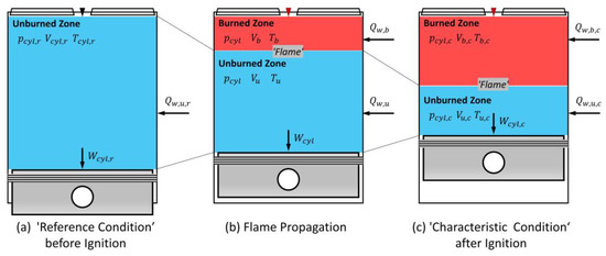
Figure 3.
Characteristic thermodynamic process of a two-zone model.
In the reference condition, as shown in Figure 3a, only the unburned zone exists in the combustion chamber. After the ignition, as shown in Figure 3b, the flame is formed, and the burned zone is generated. Then the flame continually propagates until it reaches the characteristic condition in Figure 3c.
Aiming to build the algebraic relation between the state variables in the reference condition and in the characteristic condition, as shown in Figure 4, a pseudo boundary is laid in the unburned zone. As a result, a sub-zone is isolated in the unburned zone by this pseudo boundary together with the cylinder wall and piston and renamed as pre-unburned zone (subscript “pre-u”), while the rest part of the unburned zone is also treated as a new sub-zone and renamed as pre-burned zone (subscript “pre-b”).
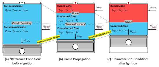
Figure 4.
Isolation of the quasi-isentropic process in the unburned zone.
The pseudo boundary can be regarded as a volume-less, frictionless, and ideally thermal conductive piston. This pseudo boundary only prevents the exchange of the mass between the pre-unburned zone and the pre-burned zone, therefore the pre-unburned zone and the pre-burned zone share the same cylinder pressure and temperature .
In the reference condition, as shown in Figure 4a, the pseudo boundary is required to guarantee the mass ratio of the gas in the pre-unburned zone over in the pre-burned zone exactly the same as the mass ratio of the gas in the unburned over in the burned zone in the ‘characteristic condition’ shown in Figure 4c, i.e.,
According to Equations (13) and (14), this mass ratio in Equation (20) is therefore calculated by the burned mass fraction , i.e.,
From Figure 4a–c, the flame gradually sweeps the pre-burned zone and finally merges with the pseudo boundary. The thermodynamic process in the pre-unburned zone can be idealized as an isentropic process under the following simplifications:
- S1: In the unburned zone, compared to the pressure-volume work , the heat transferred from the wall to the gas is ignored, which is expressed in differential-form:
- S2: The unburned zone’s heat capacity ratio , which is the ratio of the heat capacity at constant pressure over the heat capacity at constant volume , keeps constant, i.e.,
As a result, the state variables in the pre-unburned zone fulfil the following relation:
As the pre-unburned zone is not physically bounded, this idealized thermodynamic process is named the quasi-isentropic process with the prefix “quasi-“ to distinguish from the normal isentropic process, whose boundary is really bounded.
The state variables in the pre-unburned zone in the reference condition shown in Figure 4a and in the characteristic condition shown in Figure 4c fulfill Equation (24), i.e.,
In the reference condition, as shown in Figure 4a, since the pre-unburned zone and the pre-burned zone share the same cylinder pressure and temperature , the volumetric ratio is exactly same as the mass ratio of the gas between both zones, i.e.,
Due to the volumetric continuity, the total cylinder volume is the summary of the pre-unburned zone’s volume and pre-burned zone’s volume :
According to Equations (21), (26) and (27), the volume of the pre-unburned zone and the pre-burned zone in the reference condition are respectively calculated by:
Substituting Equation (28) into Equation (25), the governing equation of the quasi-isentropic process for the characteristic thermodynamic process from the reference condition to the characteristic condition is given as:
As the characteristic condition can be arbitrarily chosen in the combustion or expansion process, Equation (30) can be applied onto the whole computation domain of combustion and expansion process, therefore the universal governing equation of the quasi-isentropic process is yield, i.e.,
The governing equation of the quasi-isentropic process, Equation (31), successfully builds the algebraic relation between the state variables of the unburned zone after ignition and the state variables in the reference condition.
The governing equation of the quasi-isentropic process, Equation (31), can also be derived by integrating the unburned zone’s reduced energy conservation equation under the simplifications S1 (Equation (22)) and S2 (Equation (23)), and the step-by-step mathematical derivation can be found in Appendix B.
The algebraic-form ideal gas equation of state in the unburned zone is expressed as:
Specifying Equation (32) in the ‘reference condition’, as shown in Figure 4a, yields:
The composition of the unburned gas does not change during the simulation. Therefore, the gas constant of the unburned zone keeps constant, i.e.,
Substituting Equations (32) and (33) into Equation (34) yields:
Combining Equation (31) and Equation (35), an explicit expression for the unburned zone’s temperature is given as:
2.3. Formation of a Novel Two-Zone Model
The novel two-zone model evolves from the conventional two-zone model, whose governing equations are Equations (8)–(12), by the following two steps:
- Algebraizing the volumetric continuity (Equation (8)), the ideal gas law of state (Equation (9)), and the energy conservation equation (Equation (10)) in the unburned zone. As a result, the set of governing equations of the two-zone model becomes a set of differential-algebraic equations (DAEs).
- Decoupling the subset of the ODEs and the subset of the AEs in the governing equations of the two-zone model. As a result, the set of governing equations of the two-zone model is split into a set of ODEs and an accompanying set of AEs.
In the unburned zone, the volumetric continuity (Equation (8)) and the ideal gas law of state (Equation (9)) can be naturally expressed in algebraic-form, while the energy conservation equation (Equation (10)) can be functionally replaced by the governing equation of the quasi-isentropic process (Equation (31)). Therefore, the set of governing equations of the two-zone model can be expressed as a set of DAEs by the following 5 equations:
- The algebraic-form volumetric continuity.
- The algebraic-form ideal gas law of state in the unburned zone, Equation (32).
- The governing equation of the quasi-isentropic process, Equation (31).
- The differential-form ideal gas law of state in the burned zone, Equation (11).
- The energy conservation equation in the burned zone, Equation (12).
According to the governing equation of the isentropic process (Equation (31)), when the cylinder pressure and its derivative are given, the unburned zone’s volume and its derivative can be calculated by:
where is an intermediate variable to simplify the expression and expressed by Equation (40).
Considering the volumetric continuity (Equations (8) and (37)), the burned zone’s volume and its derivative can be calculated by:
Substituting the expression of burned zone’s volume (Equation (41)) and its derivative (Equation (42)) into Equations (11) and (12), the governing equations in the burned zone are isolated from the set of governing equations of the two-zone model and accordingly expressed by Equations (43) and (44).
As a result, the novel two-zone model is formed as a set of ODEs accompanied by a set of AEs. The set of ODEs, which numerically solves the in-cylinder pressure and burned zone’s temperature , consists of 2 equations:
- The ideal gas equation of state in the burned zone, Equation (43).
- The energy conservation equation in the burned zone, Equation (44).
This set of ODEs in the governing equations of the novel two-zone model can be written in a matrix-form linearly implicit ODE as:
where is the vector of dependent state variables and in the novel two-zone model; is the coefficient matrix; is the coefficient vector, i.e.,
The accompanying set of AEs includes Equations (36), (38), and (41), and analytically solves the burned zone’s volume , unburned zone’s volume , and temperature .
The novel two-zone model only needs solving 2 ODEs, while the conventional two-zone needs solving 5 ODEs. Obviously, the novel two-zone model is significantly simplified. Furthermore, in the novel two-zone model, solving algebraic state variables, i.e., , , and , becomes optional. It means users can choose the options: solving these state variables during or after integrating the ODEs; solving all these state variables or only a part of them. This feature makes this novel model more flexible and convenient.
2.4. Numerical Methodology
The novel two-zone model and its benchmarked models, i.e., the single-zone model and conventional two-zone model, are coded in the MATLAB computational environment, configured by the same engine specifications, and solved by the MATLAB built-in ODE solver, ode45, which is an associated Runge–Kutta method [27]. The relative error control approach is adopted in this paper and its tolerance is set at . Three thermodynamic models are evaluated from ignition to 100 °CA after TDC, which represents the combustion phase and the expansion phase in the closed part of the engine cycle. The initial conditions (subscript ‘0’) are set according to the following rules:
- The single-zone model:
- The conventional two-zone model:
- The novel two-zone modelwhere is the cylinder pressure at ignition and obtained from the experiment; is the cylinder temperature and determined by the cylinder pressure at ignition and the trapped mass of gas in cylinder according to the ideal gas equation of state; is the cylinder volume at ignition and determined by engine kinematics; is the adiabatic flame temperature at constant pressure and calculated by the method introduced by Ferguson [25].
3. Results and Discussion
The experimental data were collected from a twin-cylinder, four-stroke, liquid-cooled gasoline engine with displacement volume of 798 cc and nominal power of 66 kW at 8000 rpm, whose specifications are presented in Table 1. Four tested cases for model validation were chosen, and their locations on the engine map are shown in Figure 5.

Table 1.
Engine specifications.
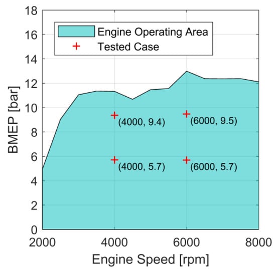
Figure 5.
Tested cases for model validation.
3.1. Model Validation
The parameters in the Wiebe function are firstly calibrated on the conventional two-zone model at each tested case and then shared by the novel two-zone model and the single-zone model. The validation results of the in-cylinder pressure and the corresponding engine conditions (engine speed, IMEP, and BMEP) are shown in Figure 6. As the Wiebe function is calibrated on the conventional two-zone model, the simulated in-cylinder pressure results from the conventional two-zone model accurately match the experimental results. Only at the high-speed cases, as shown in the scope window in Figure 6, the conventional two-zone model slightly undershoots the peak pressure. Compared to the conventional two-zone model, the single-zone model significantly overshoots the in-cylinder pressure at all tested cases. The single-zone model uses the bulk-gas temperature to calculate the wall heat transfer. As a result, the wall heat transfer is lowly estimated. The simulated cylinder pressure from the novel two-zone model well matches the results from the conventional two-zone model. Although the novel two-zone model ignores the wall heat transfer to the burned zone, the novel two-zone model remains calculating the wall heat transfer to the burned zone by the temperature of the burned gas, therefore, its performance in calculating the in-cylinder pressure is similar to the conventional two-zone model.
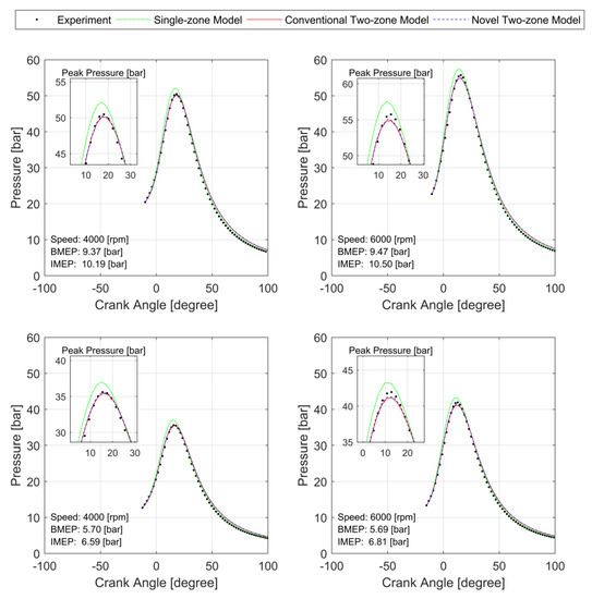
Figure 6.
Experimental and simulated in-cylinder pressure.
The novel two-zone model aims to functionally alternate the conventional two-zone model Therefore, it is necessary to evaluate its ability in calculating the unburned and burned zones’ volume and temperature against the conventional model. Figure 7 and Figure 8 respectively show the simulated volume and temperature from the conventional and the novel two-zone model. The simulated volume and temperature from the novel two-zone model well match the results from the conventional model at all tested cases. Therefore, the novel two-zone model is proved as a qualified alternative to the conventional two-zone model.
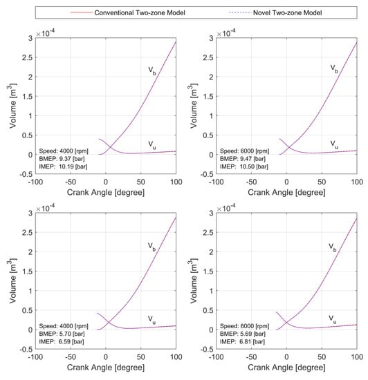
Figure 7.
Simulated volume from conventional and novel two-zone model.
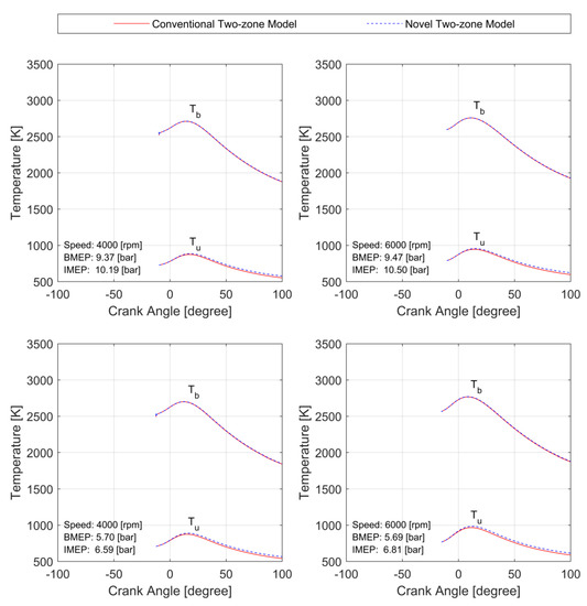
Figure 8.
Simulated temperature from conventional and novel two-zone model.
3.2. Model Stiffness
The governing equations for the single-zone model (Equation (4)), the conventional two-zone model (Equation (16)) and the novel two-zone model (Equation (45)) share a universal form by Equation (52).
The explicit form governing equation of the thermodynamic models can be linearized at the simulation step as:
where is the Jacobian matrix of with respect to the vector of dependent state variables and numerically calculated by the finite difference method.
The stiffness ratio is defined as the ratio between the maximal and the minimal magnitude of the eigenvalue of the Jacobian matrix of [28], i.e.,
where denotes the magnitude; denotes the real part of an eigenvalue of the Jacobian matrix of .
The stiffness ratio is an indicator to measure the stiffness of an ODE system [28], and its local values for the single-zone model, conventional two-zone model, and the novel two-zone model are shown in Figure 9. The single-zone model has the lowest stiffness of these three models. As a result, the single-zone model is possible to be solved at the longest simulation steps, which is represented in Figure 10. In contrast, the conventional two-zone model has the highest stiffness among these three models. Due to the high stiffness, the simulation steps must be shortened to achieve sound solutions for the conventional two-zone model, which can be seen in Figure 10. Particularly, the conventional two-zone model behaves extremely stiffly at the initial stage of the simulation, because the burned zone is too small, therefore sufficiently sensitive to the heat flux. When the burned zone grows, the stiffness of the conventional two-zone model declines, however, the model stiffness still stays on the high level after the burned zone has well developed due to the complex model structure. The novel two-zone model meets the same problem at the initial stage of the simulation such as the conventional two-zone model, but its model stiffness is significantly reduced because its governing equations in the burned zone have been partially algebraized. Similar to the conventional two-zone model, along with the growth of the burned zone, the stiffness of the novel two-zone model sharply declines to the level of the single-zone model, therefore, the novel two-zone model can be solved at the simulation steps with similar length as the single-zone model, which is shown in Figure 10.
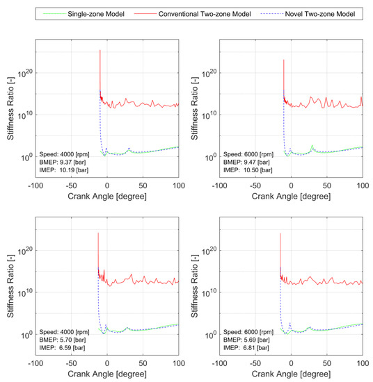
Figure 9.
Stiffness ratio.
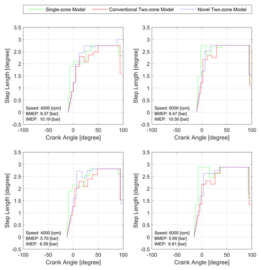
Figure 10.
Simulation step length.
3.3. Analysis of Error Due to Simplifications
According to the mathematical derivation (given in Appendix B) from the energy conservation equation (Equation (10)) to the governing equation of the quasi-isentropic (Equation (31)) in the unburned zone of a two-zone model, the proposed simplifications, S1 (Equation (22)) and S2 (Equation (23)), essentially simplify the expressions of 2 terms in the energy conservation equation. Therefore, the errors resulting from these simplifications can be identified and evaluated by investigating the behaviors of these simplified terms during the mathematical derivation.
Simplification S1 says, compared to the pressure-volume work, the heat transferred from the wall to the gas in the unburned zone is ignored, i.e., . This simplification is applied on Equation (A18) at the 9th step of the mathematical derivation (Appendix B) and yields the simplified expression, Equation (A19). Simplification S1 essentially replaces in Equation (A18) by in Equation (A19). Accordingly, a relative error of the simplification S1 is defined by Equation (55).
This relative error only evaluates the influence made by the Simplification S1 on the coefficient of the term in Equation (A18). Obviously, when the volumetric derivative of the unburned zone moves close to zero, the relative error tends to infinity; however, their product simultaneously tends to zero. In other words, though the relative error grows when the volumetric derivative of the unburned zone goes towards zero, the relative error is diluted and not completely transferred to the simplified expression (Equation (A19)). In order to include this dilution effect, a dimensionless parameter is introduced in the definition expression of the relative error (Equation (55)), and is the maximum of the absolute volumetric derivative of the unburned zone , i.e., . As a result, the definition of the relative error of S1 is modified to:
Figure 11 represents the derivative of unburned zone’s transferred heat and pressure-volume work together with the relative error of S1 . As shown in Figure 11, derivative of pressure-volume work is close to zero compared with the derivative of transferred heat . As a result, the relative error of S1 is small (less than 0.6) and significantly diluted along with the slowing change of the unburned zone’s volume (shown in Figure 7).
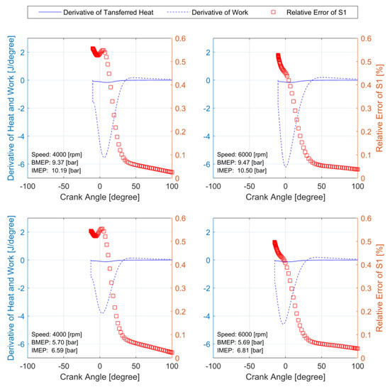
Figure 11.
Derivative of heat transferred to wall and pressure-volume work in unburned zone together with the relative error of simplification S1.
Simplification S2 is applied on Equation (A19) at the 10th step of the mathematical derivation (Appendix B) to convert Equation (A19) to an ODE with constant coefficients. This simplification treats the unburned zone’s heat capacity ratio as a constant value, and this constant value is specified as its initial value during the simulation. Therefore, a relative error of the simplification S2 is defined by Equation (57).
Figure 12 represents the unburned zone’s heat capacity ratio and the relative error of S2. The fluctuation of heat capacity ratio is small and the relative errors of S2 are bounded in .
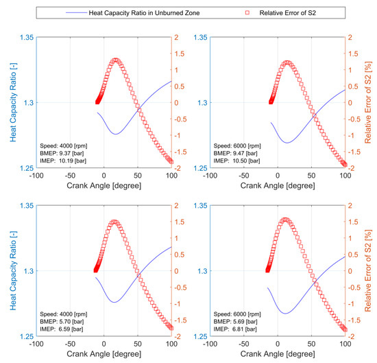
Figure 12.
Heat capacity ratio of unburned zone together with the relative error of simplification S2.
4. Conclusions
This paper isolates a thermodynamic process in the unburned zone of a two-zone model and proposes two simplifications to idealize this thermodynamic process as a ‘quasi-isentropic process’, and accordingly derives the governing equation of this quasi-isentropic process. As a result, the governing equation of the quasi-isentropic process successfully builds the algebraic relation between the state variables of the unburned zone after ignition and the state variables in a ‘reference condition’ before the ignition.
The governing equation of the quasi-isentropic process is mathematically derived by integrating the reduced energy conservation equation of the unburned zone. Along with this mathematical derivation, the proposed simplifications simplify the expressions of the energy conservation equation of the unburned zone, thus leading to some errors in solving the energy conservation equation of the unburned zone. However, the results of error analysis show the errors caused by the proposed simplifications are small, therefore, the simplifications are acceptable.
Based on the quasi-isentropic process, this paper decouples the governing equations in the burned zone from the governing equations in the unburned zone and accordingly forms a novel two-zone model as a set of 2 ODEs accompanied by a set of 3 AEs. The model structure of the novel two-zone model is similarly complex as the single-zone model while much simpler than the conventional two-zone model. As a result, the stiffness of the novel two-zone model is much lower than the conventional two-zone model at all the tested cases and even declines to the level of the single-zone model when the burned zone has well developed. Meanwhile, according to the validation results, the novel two-zone model maintains high accuracy in calculating state variables such as the conventional two-zone model.
To conclude, the novel two-zone model inherits the conventional two-zone model’s ability to accurately estimate both zones’ state variables while its simplified structure reduces its stiffness down to the level of the single-zone model. Therefore, the novel two-zone model is especially suited for applying in computationally intensive scenarios, e.g., numerical optimal control, model-based engine-calibration, and control design.
Funding
This research was a part of the doctoral program of the author (Y.W.), which was founded by China Scholarship Council, grant number 201606250012. The Open Access Publishing of this paper was founded by Graz University of Technology.
Acknowledgments
The author expresses his gratitude to Stephan Schmidt, Stephan Jandl, and Christian Zinner for their valuable scientific and editorial comments and for proof-reading the paper, and to Katherine Tiede for her writing assistance. The author thanks China Scholarship Council for granting him a Ph.D. research scholarship.
Conflicts of Interest
The authors declare no conflict of interest.
Appendix A. Sub-Models of the Thermodynamic Model
Appendix A.1. Engine Kinematics
The instantaneous cylinder volume is a function of crank angle which follows from the engine geometry:
where is the clearance volume; is the cylinder bore; is the connecting rod length; is the crank radius.
Appendix A.2. Burned Mass Fraction—Wiebe Function
The burned mass fraction , which is defined as the ratio of the mass of burned gas to the mass of total trapped gas in cylinder , is modelled as Wiebe function [29] in this paper, i.e.,
where is the crank angle at the start of combustion; is the duration of total combustion; and are the tuning parameters.
Appendix A.3. Heat Transfer
Resulting mainly due to the forced convection [30], the heat rate transferred from the cylinder wall to the zone in the combustion chamber follows the Newton’s law of cooling, i.e.,
where is the angular velocity of the crank angle ; is the temperature of the cylinder wall; is the temperature of the gas in zone ; is the heat transfer coefficient and determined by the Woschni correlation [26]; is the instantaneous surface area. For the single-zone model, the instantaneous surface area is determined by the engine kinematics and can be calculated by Equation (A4). For the two-zone model, Equations (A5) and (A6), which are proposed by Ferguson [25], are used to calculate the instantaneous surface area of unburned zone and burned zone.
Appendix A.4. Chemical Composition and Thermodynamic Property
Consider the combustion reaction:
Two types of the gas models are adopted in this paper:
- Unburned gas, as shown at the left-hand-side of Equation (A7), is a homogeneous mixture of the fuel () and the air ( and ), and its composition is determined by the fuel-air equivalence ratio .
- Burned gas, as shown at the right-hand-side of Equation (A7), is a homogeneous mixture of 11 combustion products (, , , , , , , , , , ) at chemical equilibrium (at the temperature of the zone and the uniform cylinder pressure) [31].
Considering four atom-balance equations () and seven chemical equilibrium reactions (Equation (A8)) [31], the molar fraction of the burned gas , along with its partial derivative with respect to pressure and to temperature , can be calculated by the method introduced by Rakopoulos et al. [32]. (n refers to a certain combustion product.)
The thermodynamic properties of the mixture (e.g., specific enthalpy, specific internal energy, specific heat capacity at constant pressure, and their partial derivatives with respect to pressure/temperature), needed by the presented thermodynamic models during the simulation, can be calculated according to the molar fraction of each species and thermodynamic properties of species based on the gas mixture rule. For the thermodynamic properties of species, the specific heat at constant pressure, the specific enthalpy and the specific entropy are calculated by NASA 7-coefficients polynomial expressions [33], and then the other thermodynamic properties of species can be derived from the known thermodynamic properties (See detailed derivation in reference [25]).
In the two-zone model, the unburned zone is filled with unburned gas, while the burned zone is filled with burned gas. However, in the single-zone model, there is only one zone in the combustion chamber. As there exist both the unburned gas and burned gas in one zone, neither the unburned gas nor burned gas can represent well the thermodynamic behaviors of the cylinder content when they are only simply applied. As a result, a method introduced by Depcik et al. [34] is used to calculate the gross thermodynamic property of the cylinder content. A thermodynamic property is respectively calculated based on unburned gas model and burned gas model, then the gross thermodynamic property of the cylinder content is the weighted average of the both results according to the burned mass fraction .
Appendix B. Mathematical Derivation of the Governing Equation of the Quasi-Isentropic Process
In the unburned zone of the two-zone model, the governing equation of the quasi-isentropic process (Equation (31)) can be derived from the ideal gas law of state (Equation (9)) and the energy conservation equation (Equation (10)) by the following steps:
- Multiplying Equation (9) by the heat capacity at constant volume yields Equation (A9).
- Multiplying Equation (10) by the gas constant yields Equation (A10).
- Summing Equations (A9) and (A10) side-by-side yields Equation (A11).
- Substituting Equation (A12) into Equation (A11) yields Equation (A13).
- Substituting unburned zone’s algebraic-form ideal gas law of state (Equation (A14)) into Equation (A13) yields Equation (A15).
- Substituting the expression of unburned zone’s mass (Equation (14)) and its derivative (Equation (15)) into Equation (A15) yields Equation (A16).
- Dividing Equation (A16) by yields Equation (A17).
- Rearranging Equation (A17) yields Equation (A18).
- Applying the simplification S1 (Equation (22) on Equation (A18) yields Equation (A19).
- Applying the simplification S2 (Equation (23)) on Equation (A19) converts Equation (A19) to an ODE with constant coefficients.
- Integrating Equation (A19) yields Equation (A20).
- To obtain the constant in Equation (A20), applying Equation (A20) in its initial condition (Equation (A21)), i.e., the ‘reference condition’ shown in Figure 4a, yields Equation (A22).
- Exponentiating Equation (A22) finally derives the governing equation of the quasi-isentropic process Equation (31).
Nomenclature
| area | |
| crank radius | |
| cylinder bore | |
| heat capacity at constant pressure | |
| heat capacity at constant volume | |
| enthalpy | |
| connecting rod length | |
| mass | |
| pressure | |
| heat | |
| gas constant | |
| temperature | |
| , | internal energy |
| volume | |
| clearance volume | |
| pressure-volume work | |
| burned mass fraction | |
| Subscript | |
| initial value | |
| cylinder | |
| target zone | |
| surrounding zone | |
| unburned zone | |
| burned zone | |
| pre-unburned zone | |
| pre-burned zone | |
| reference condition before ignition | |
| characteristic condition after ignition | |
| combustion | |
| compression | |
| wall | |
| single-zone model | |
| conventional two-zone model | |
| novel two zone model | |
| Wiebe function | |
| Greek symbols | |
| crank angle | |
| angular velocity of crank angle | |
| fuel-air equivalence ratio | |
| heat capacity ratio | |
| vector of dependent state variables | |
| coefficient matrix | |
| coefficient vector | |
| eigenvalue | |
| coefficient | |
| Abbreviation | |
| AE | Algebraic Equation |
| BMEP | Brake Mean Effective Pressure |
| CO | Carbon Monoxide |
| HiL | Hardware in the Loop |
| IMEP | Indicated Mean Effective Pressure |
| NOx | Nitrogen Oxides |
| ODE | Ordinary Differential Equation |
| LHV | Lower Heating Value |
| Notation | |
| derivative of with respect to crank angle/time | |
| partial derivative of | |
| magnitude of | |
| inverse of matrix |
References
- Hatami, M.; Cuijpers, M.C.M.; Boot, M.D. Experimental optimization of the vanes geometry for a variable geometry turbocharger (VGT) using a Design of Experiment (DoE) approach. Energy Convers. Manag. 2015, 106, 1057–1070. [Google Scholar] [CrossRef]
- Abd-Alla, G.H. Using exhaust gas recirculation in internal combustion engines: A review. Energy Convers. Manag. 2002, 43, 1027–1042. [Google Scholar] [CrossRef]
- Gao, J.; Wu, Y.; Shen, T. On-line statistical combustion phase optimization and control of SI gasoline engines. Appl. Therm. Eng. 2017, 112, 1396–1407. [Google Scholar] [CrossRef]
- Finesso, R.; Spessa, E. A real time zero-dimensional diagnostic model for the calculation of in-cylinder temperatures, HRR and nitrogen oxides in diesel engines. Energy Convers. Manag. 2014, 79, 498–510. [Google Scholar] [CrossRef]
- Benajes, J.; García, A.; Monsalve-Serrano, J.; Martínez-Boggio, S. Optimization of the parallel and mild hybrid vehicle platforms operating under conventional and advanced combustion modes. Energy Convers. Manag. 2019, 190, 73–90. [Google Scholar] [CrossRef]
- Ngayihi Abbe, C.V.; Nzengwa, R.; Danwe, R.; Ayissi, Z.M.; Obonou, M. A study on the 0D phenomenological model for diesel engine simulation: Application to combustion of Neem methyl esther biodiesel. Energy Convers. Manag. 2015, 89, 568–576. [Google Scholar] [CrossRef]
- Rakopoulos, C.D.; Michos, C.N. Development and validation of a multi-zone combustion model for performance and nitric oxide formation in syngas fueled spark ignition engine. Energy Convers. Manag. 2008, 49, 2924–2938. [Google Scholar] [CrossRef]
- Nilsson, Y.; Eriksson, L. A New Formulation of Multi-Zone Combustion Engine Models. IFAC Proc. Vol. 2017, 34, 357–362. [Google Scholar] [CrossRef]
- Maroteaux, F.; Saad, C.; Aubertin, F. Development and validation of double and single Wiebe function for multi-injection mode Diesel engine combustion modelling for hardware-in-the-loop applications. Energy Convers. Manag. 2015, 105, 630–641. [Google Scholar] [CrossRef]
- Verhelst, S.; Sheppard, C.G.W. Multi-zone thermodynamic modelling of spark-ignition engine combustion—An overview. Energy Convers. Manag. 2009, 50, 1326–1335. [Google Scholar] [CrossRef]
- Maroteaux, F.; Saad, C. Combined mean value engine model and crank angle resolved in-cylinder modeling with NOx emissions model for real-time Diesel engine simulations at high engine speed. Energy 2015, 88, 515–527. [Google Scholar] [CrossRef]
- Neshat, E.; Honnery, D.; Saray, R.K. Multi-zone model for diesel engine simulation based on chemical kinetics mechanism. Appl. Therm. Eng. 2017, 121, 351–360. [Google Scholar] [CrossRef]
- Song, E.; Shi, X.; Yao, C.; Li, Y. Research on real-time simulation modelling of a diesel engine based on fuel inter-zone transfer and an array calculation method. Energy Convers. Manag. 2018, 178, 1–12. [Google Scholar] [CrossRef]
- Maroteaux, F.; Saad, C. Diesel engine combustion modeling for hardware in the loop applications: Effects of ignition delay time model. Energy 2013, 57, 641–652. [Google Scholar] [CrossRef]
- Gambarotta, A.; Lucchetti lng, G. Control-Oriented “Crank-Angle” Based Modeling of Automotive Engines. SAE Tech. Pap. Ser. 2011, 1, 16. [Google Scholar] [CrossRef]
- Corti, E.; Migliore, F.; Moro, D.; Capozzella, P.; Pagano, M. Development of a control-oriented model of engine, transmission and vehicle systems for motor scooter HIL testing. SAE Tech. Pap. 2009, 4970, 12. [Google Scholar] [CrossRef]
- D’Errico, G. Prediction of the combustion process and emission formation of a bi-fuel s.i. engine. Energy Convers. Manag. 2008, 49, 3116–3128. [Google Scholar] [CrossRef]
- Rakopoulos, C.D.; Rakopoulos, D.C.; Giakoumis, E.G.; Kyritsis, D.C. Validation and sensitivity analysis of a two zone Diesel engine model for combustion and emissions prediction. Energy Convers. Manag. 2004, 45, 1471–1495. [Google Scholar] [CrossRef]
- Savva, N.; Hountalas, D. Detailed evaluation of a new semi-empirical multi-zone NOx model by application on various diesel engine configurations. SAE Tech. Pap. 2012, 1–17. [Google Scholar] [CrossRef]
- Provataris, S.A.; Savva, N.S.; Chountalas, T.D.; Hountalas, D.T. Prediction of NOx emissions for high speed DI Diesel engines using a semi-empirical, two-zone model. Energy Convers. Manag. 2017, 153, 659–670. [Google Scholar] [CrossRef]
- Chindaprasert, N.; Hassel, E.; Nocke, J.; Janssen, C.; Schultalbers, M.; Magnor, O. Prediction of co emissions from a gasoline direct injection engine using chemkin®. SAE Tech. Pap. 2006. [Google Scholar] [CrossRef]
- Soylu, S. Prediction of knock limited operating conditions of a natural gas engine. Energy Convers. Manag. 2005, 46, 121–138. [Google Scholar] [CrossRef]
- Manivel, R.; Dhandapani, S. Two Zone Combustion Modelling of Two Stroke Spark Ignited Catalytic Engine. SAE Tech. Pap. 2001, 2001-Janua, 297–302. [Google Scholar] [CrossRef]
- Caton, J. An Introduction to Thermodynamic Cycle Simulations for Internal Combustion Engines; John Wiley & Sons, Ltd Registered: Hoboken, NJ, USA, 2016; ISBN 9781119037569. [Google Scholar]
- Ferguson, C.; Kirkpatrick, A. Internal Combustion Engines: Applied Thermosciences; John Wiley & Sons, Ltd Registered: Hoboken, NJ, USA, 2015; ISBN 978-1-118-53331-4. [Google Scholar]
- Lounici, M.S.; Loubar, K.; Balistrou, M.; Tazerout, M. Investigation on heat transfer evaluation for a more efficient two-zone combustion model in the case of natural gas SI engines. Appl. Therm. Eng. 2011, 31, 319–328. [Google Scholar] [CrossRef]
- Ashino, R.; Nagase, M.; Vaillancourt, R. Behind and Beyond the MATLAB ODE Suite. Comput. Math. Appl. 2000, 40, 491–512. [Google Scholar] [CrossRef]
- Spijker, M.N. Stiffness in numerical initial-value problems. J. Comput. Appl. Math. 1996, 72, 393–406. [Google Scholar] [CrossRef]
- de Faria, M.M.N.; Vargas Machuca Bueno, J.P.; Ayad, S.M.M.E.; Belchior, C.R.P. Thermodynamic simulation model for predicting the performance of spark ignition engines using biogas as fuel. Energy Convers. Manag. 2017, 149, 1096–1108. [Google Scholar] [CrossRef]
- Nefischer, A.; Neumann, J.; Stanciu, A.; Wimmer, A. Quasi-dimensional modelling of turbulence-driven phenomena in SI engines. Int. J. Veh. Des. 2014, 66, 297. [Google Scholar] [CrossRef]
- Rakopoulos, C.D.; Michos, C.N. Quasi-dimensional, multi-zone combustion modelling of turbulent entrainment and flame stretch for a spark ignition engine fuelled with hydrogen-enriched biogas. Int. J. Veh. Des. 2009, 49, 3. [Google Scholar] [CrossRef]
- Rakopoulos, C.D.; Hountalas, D.T.; Tzanos, E.I.; Taklis, G.N. A fast algorithm for calculating the composition of diesel combustion products using 11 species chemical equilibrium scheme. Adv. Eng. Softw. 1994, 19, 109–119. [Google Scholar] [CrossRef]
- Mcbride, B.; Gordon, S.; Reno, M. Coefficients for Calculating Thermodynamic and Transport Properties of Individual Species. Nasa Tech. Memo. 1993, 4513, 98. [Google Scholar]
- Depcik, C.; Jacobs, T.; Hagena, J.; Assanis, D. Instructional use of a single-zone, premixed charge, spark-ignition engine heat release simulation. Int. J. Mech. Eng. Educ. 2007, 35, 1–31. [Google Scholar] [CrossRef]


© 2020 by the author. Licensee MDPI, Basel, Switzerland. This article is an open access article distributed under the terms and conditions of the Creative Commons Attribution (CC BY) license (http://creativecommons.org/licenses/by/4.0/).