Comparative Study of CFD and LedaFlow Models for Riser-Induced Slug Flow

Abstract

The goal of this study is to compare mainstream Computational Fluid Dynamics (CFD) with the widely used 1D transient model LedaFlow in their ability to predict riser induced slug flow and to determine if it is relevant for the offshore oil and gas industry to consider making the switch from LedaFlow to CFD. Presently, the industry use relatively simple 1D-models, such as LedaFlow, to predict flow patterns in pipelines. The reduction in cost of computational power in recent years have made it relevant to compare the performance of these codes with high fidelity CFD simulations. A laboratory test facility was used to obtain data for pressure and mass flow rates for the two-phase flow of air and water. A benchmark case of slug flow served for evaluation of the numerical models. A 3D unsteady CFD simulation was performed based on Reynolds-Averaged Navier-Stokes (RANS) formulation and the Volume of Fluid (VOF) model using the open-source CFD code OpenFOAM. Unsteady simulations using the commercial 1D LedaFlow solver were performed using the same boundary conditions and fluid properties as the CFD simulation. Both the CFD and LedaFlow model underpredicted the experimentally determined slug frequency by 22% and 16% respectively. Both models predicted a classical blowout, in which the riser is completely evacuated of water, while only a partial evacuation of the riser was observed experimentally. The CFD model had a runtime of 57 h while the LedaFlow model had a runtime of 13 min. It can be concluded that the prediction capabilities of the CFD and LedaFlow models are similar for riser-induced slug flow while the CFD model is much more computational intensive.

1. Introduction

The accurate prediction of the two-phase flow in riser pipeline systems are important for the design and process control of offshore oil and gas facilities [1,2]. The 1D commercial code LedaFlow is commonly used in the industry to predict the undesired slug formation and peak pressure levels [3]. Advances in available computational resources have made it possible to consider using higher-fidelity 3D codes based on Computational Fluid Dynamics (CFD), instead.

Slug flow is a two-phase phenomenon of transient nature and therefore difficult to predict using analytical approaches [4]. Riser-induced slug flow is undesired in the process system because it leads to highly fluctuating flow and pressure levels, which can lead to poor separator performance among others [5]. The phenomenon of riser-induced slug flow is caused by the heavier liquid phase building up at geometrical low points in the riser, blocking the gas flow. 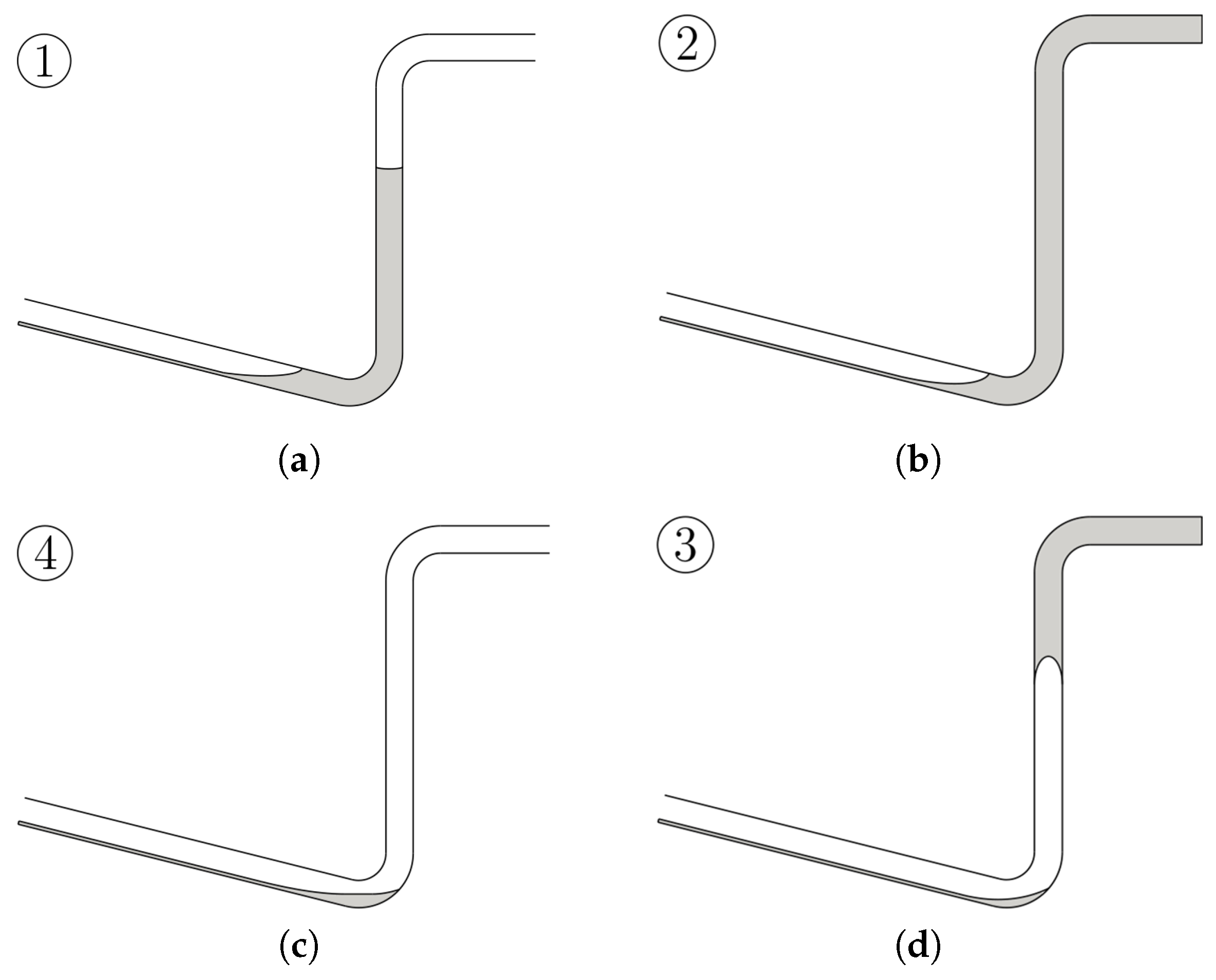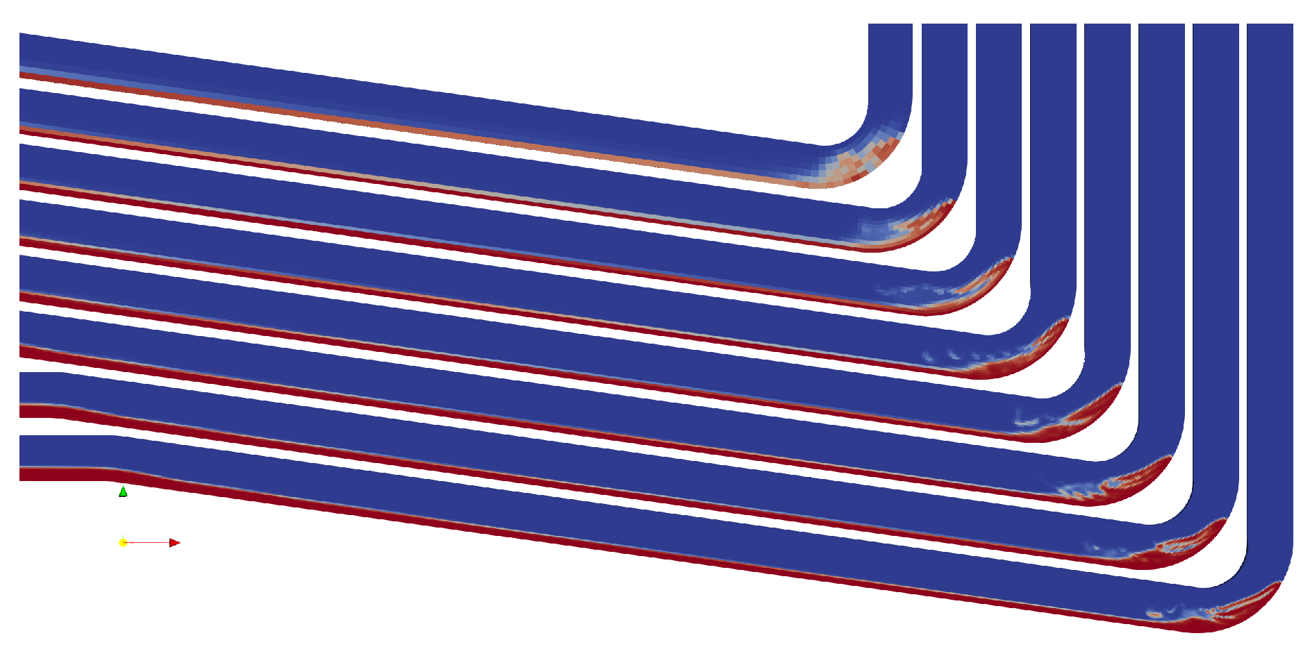Figure 1 shows the stages of a riser-induced slug cycle starting at top left. The cycle has a constant frequency which is influenced by the current flow parameters.

• Slug formation—The slug starts forming at the bottom of the riser. As liquid blocks the pipe, the upstream gas pressure increases.
• Slug production—As the slug reaches the top of the riser, liquid is transported to the separator.
• Blowout—The compressed gas reaches the bottom of the riser as the gas pressure exceeds the gravitational head of the slug. The gas expands up the riser and causes an acceleration of the liquid slug.
• Liquid fallback—Residual liquid falls to the bottom of the riser to restart the cycle.

The topic of gas-liquid slug flow have most recently been reviewed by Morgado et al. [6] who underlined the need for more experimental confirmation of numerical models. Presently, dynamic 1D models to predict the complex two phase flow pattern in offshore pipelines are based on the unit cell concept which was originally proposed by Wallis [7]. Research within these mechanistic models are focused on improving the closure relations to advance the prediction capabilities without significantly increasing the complexity of the solution [8]. This is most recently demonstrated by Soedarmo et al. [9] who suggested a new ad-hoc closure relationship for intermittent flow in pipes and by Fan et al. [10] who suggested a new model based on dimensional predictive regression. Models based on the unit cell concept are attractive as they only require very few computational resources, however it is well known that only CFD models can possibly correctly predict the complex physics of slug flow [11].

The numerical solution of the governing equations of fluid flow with spatial and temporal resolution of bubbles and turbulence is known as CFD. To model two-phase flow the Volume Of Fluid (VOF) method is most often used to resolve the gas-liquid interface. The VOF model have prove to be superior compared to other two-phase models for vertical flow [12] and have been validated for vertical slug flow using experimental data [13]. The VOF model have also been shown to be capable of predicting the full spectrum of flow pattern, such as stratified, wavy, slug, plug and annular flows [14,15]. Thus, the accurate simulation of the physics of the flow field using CFD can be used to give a better understanding of the transition between the different flow patterns [16,17]. 3D CFD simulations have also been used to directly provide input for the development of closure relationships [18]. Thus, the use of CFD enables the user to perform accurate predictions on the detailed dynamics of two-phase flow without the need to invest in expensive in-situ experimental tests [19]. 3D CFD simulations are able to predict non-symmetric nature of the interface shape and are thus able to capture flow phenomenon which cannot be modelled by 1D techniques [20]. CFD models for multiphase flow are also continuously developed to include new features such as Fluid Structure Interaction [21] and more accurate prediction of the gas liquid interface [22].

Previous studies have shown that there is a continuous efforts towards improving mechanistic models as well as CFD simulations using the VOF model. The aim of this study is to directly compare the prediction performance of these two models as well as their computational cost. By comparing objective parameters such as the predicted slug frequency and maximum pressure against newly acquired experimental data it is possible to make an informed choice whether to use high fidelity, but more computational intensive CFD models, compared to existing mechanistic 1D models.

In this study, two models have been developed and evaluated against experimental data acquired at the laboratory facility located in Aalborg University, Esbjerg campus. Models are developed through 1D approaches using the commercial software LedaFlow, while a more complex 3D CFD model is developed within the open source framework of OpenFOAM v6. The benefit of 1D modeling is the reduction in computational cost, while the appeal of 3D modeling is the potential improvement of modeling accuracy. Although the strong and weak points of both modeling principles are already known it is rarely quantified how big the deviations are in the key parameters characterizing the slug flow; this study focuses on comparing the models where the main evaluation is based on quantification of slug progression and period as well as the computational time.

In this article, the experimental facility and its setup is presented in Section 2. This includes physical properties of the facility and the given operating conditions of which the numerical models are based upon. In Section 3, the developed numerical models for both CFD and 1D simulations are addressed in terms of the chosen meshing strategies, discretization schemes and fluid and turbulence models. In Section 4, the numerical results and experimental data are presented and compared using pressure plots of the riser topside and low-point over time, together with the topside mass flow over time. The performance of the numerical models is evaluated based on the correlation with experimental data in terms of peak pressures and slug frequency, the ability to predict phase interfaces and their computational intensity. Finally, in Section 5, the article is concluded through summarizing the main findings of the present work.

2. Experimental Method

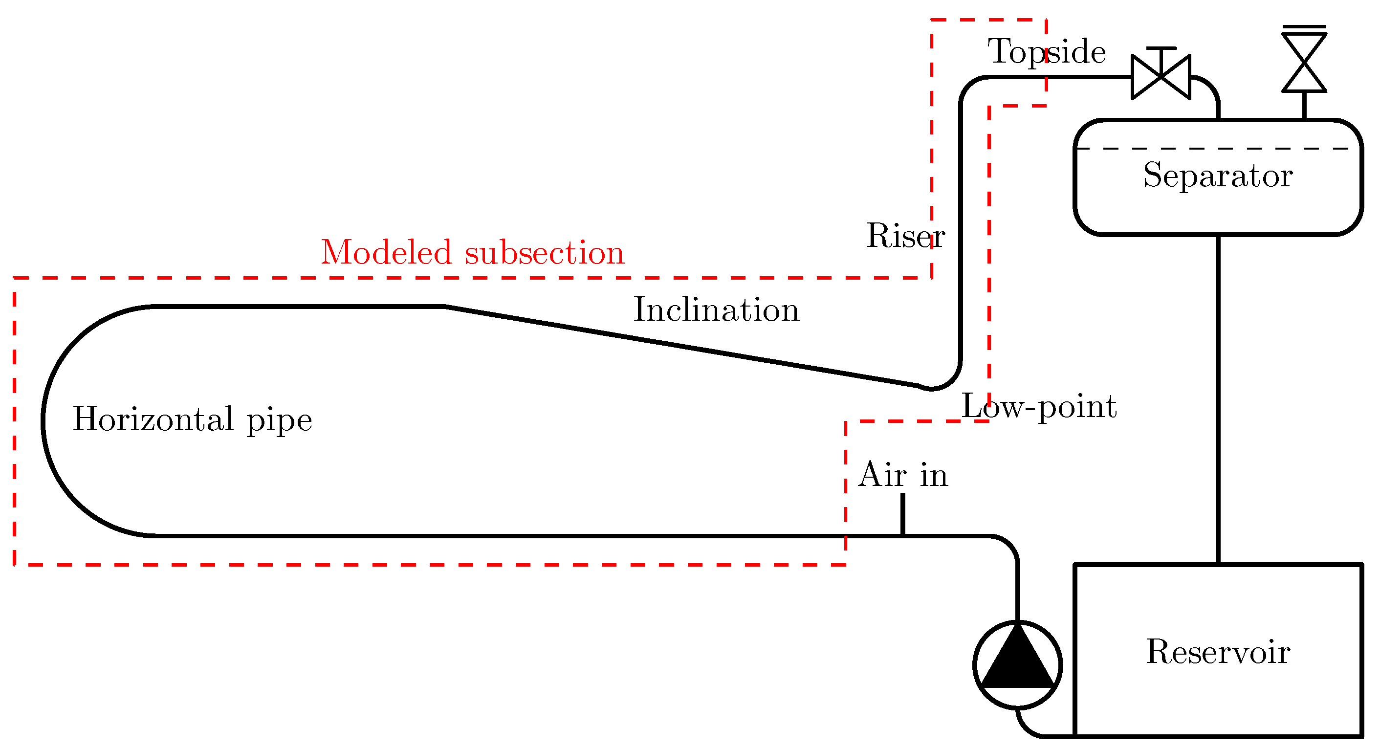
A process diagram for the test facility, including pipe section designations, is presented in Figure 2. Water is recirculated in the system by a pump while air is injected immediately after the recirculation pump and removed in the two-phase separator. The setup is more thoroughly described in Reference [23,24] while selected dimensions are presented in 

Table 1. Dimensions of the test facility pipeline.

Parameter	Symbol	Value
Pipe material	-	PVC
Pipe diameter	D	0.051 m
Horizontal pipeline length	$l_{\mathrm{h}}$	30 m
Inclination length	$l_{\mathrm{i}}$	12 m
Riser length	$l_{\mathrm{r}}$	6 m
Inclination angle	$\beta$	$-8^{\circ }$
Material roughness	$\epsilon$	1.5 × 10${}^{-6}$ m

.

Pressure and temperature transmitters are located along the pipes. The Siemens SITRANS P200 7MF1565 pressure transmitters at the low-point, $p_{\mathrm{rb}}$, and topside, $p_{\mathrm{rt}}$, are placed as presented in Figure 3. A bespoke Micro Motion ELITE Coriolis flow meter utilizing a CFM200M transmitter, capable of measuring both mass flow and density, is installed topside. The flow rate entering the separator is indicated with the symbol ${\omega }_{\mathrm{sep},\mathrm{in}}$. The flow meter is developed for single-phase flow but is designed to reduce inaccuracy in two-phase flow. The topside choke valve is maintained fully open during the experiment. The actuators and transmitters are described in details in Reference [25].

The experimental configuration presented in 

Table 2. Experimental test results. Volumes are stated for normal conditions.

Parameter	Symbol	Value
Separator pressure	$p_{\mathrm{sep}}$	103 kPa
Temperature, avg.	T	22 ${}^{\circ }$C
Liquid nominal avg. mass flow	${\omega }_{\mathrm{L},\mathrm{in}}$	0.4 kg/s
Gas nominal avg. volume flow	${\omega }_{\mathrm{G},\mathrm{in}}$	1.25 ${\mathrm{Nm}}^3/\mathrm{h}$
Topside valve opening	-	100%
Slug frequency	$f_{\mathrm{slug}}$	1/78.5 Hz

is based on Scenario 1, Test 1 of Reference [26]. The Table shows the input parameters and results of the laboratory test with averaged values as all parameters varies insignificantly with regards to change in fluid properties. The setpoint for the separator mass flow is 0.4 kg/s. The slug frequency is estimated from Fast Fourier Transform (FFT) analysis.

The setup is replicated, and new data is recorded. This includes the low-point pressure and topside pressure and mass flow for the first 350 s after the initial transient slug cycle. The sampling rate is 100 Hz to ensure flow dynamics of interest is captured.

3. Numerical Methods

The software used for 1D modeling in this study is LedaFlow Engineering v2.4.255.030, referenced simply as LedaFlow. Alternative softwares with similar features include OLGA; however, previous studies have shown that for the simulation of riser-induced slug flow, LedaFlow and OLGA perform comparably, with same strong and weak point [3]. In Figure 4, the LedaFlow simulation setup is presented using the LedaFlow interface.

Each flow component requires specification of several parameters within the categories: INLET, OUTLET, PIPELINE, VALVE and LOSS. The parameters are listed in 

Table 3. Simulation model setup for LedaFlow.

	Parameter	Value	Unit
INLET	Mass flow rate, water	0.4	kg/s
	Mass flow rate, air	$449\times {10}^{-6}$	kg/s
OUTLET	Pressure	103	kPa
	Temperature	295	K
	Volume fraction, water	0	-
	Volume fraction, air	1	-
PIPELINE	Thickness	7.75	mm
	Roughness	$1.5\times {10}^{-6}$	m
	Heat capacity	1000	$\mathrm{J}/\left(\mathrm{kgK}\right)$
	Thermal conductivity	0.19	$\mathrm{W}/\left(\mathrm{mK}\right)$
	Density	1390	$\mathrm{kg}/{\mathrm{m}}^3$
VALVE	Opening	1	-
	Discharge coefficient	0.84	-
LOSS	$k_{\mathrm{L}}$, 8${}^{\circ }$ bend	0.6	-
	$k_{\mathrm{L}}$, 98${}^{\circ }$ bend w. $r/D=10$	0.57	-
	$k_{\mathrm{L}}$, 90${}^{\circ }$ bend w. $r/D=1.5$	0.3	-
	$k_{\mathrm{L}}$, Globe valve, fully open	6.5	-

.

For Pressure Volume Temperature (PVT) settings, the user has the option to either use a PVT table or use constant PVT values defined by the user. As the experimental temperature change is insignificant and the total pressure change is not expected to exceed 2 bar, it is considered acceptable to use constant values instead of PVT tables. Thus, the constant values for air and water are implemented in LedaFlow.

3D Model

The solver used for this case is the standard solver compressibleInterFoam of OpenFOAM v6. The model is developed for two compressible, non-isothermal, immiscible fluids using the VOF method [27]. The model solves transport equations for continuity, the Reynolds Averaged Navier Stokes (RANS), volume fraction, turbulent kinetic energy, k, and the dissipation rate, $\epsilon$, as they are implemented in the OpenFOAM v6 code.

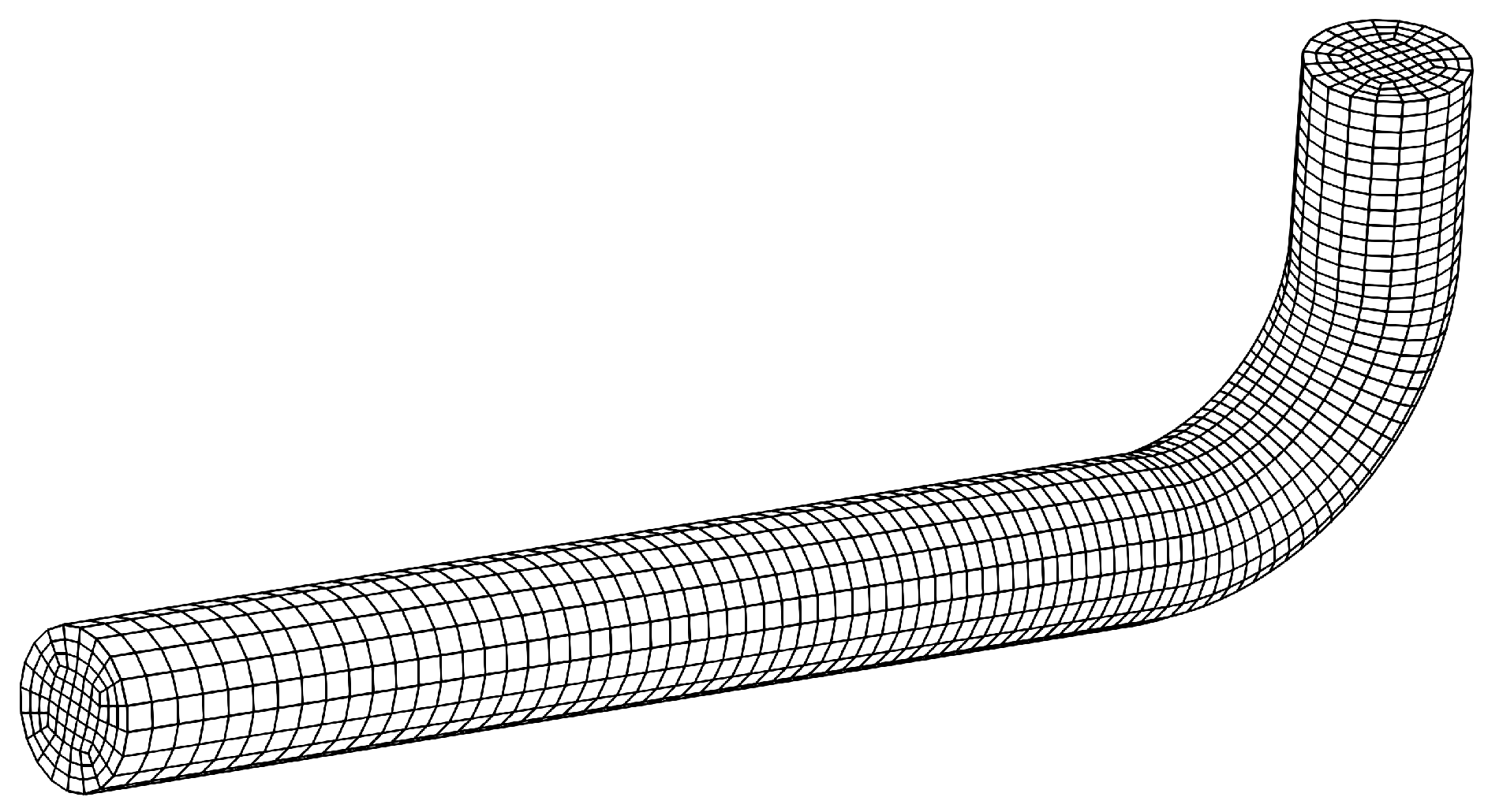
For high mesh quality, a hexahedral butterfly mesh was developed, of which an excerpt is presented in Figure 5. A grid independency analysis was performed to determine an adequate mesh resolution evaluated based on interface resolution and the riser bottom pressure progress. The total cell count of the final mesh is 240 k.

Four boundaries are specified; water inlet, air inlet, outlet and wall. Inlets are specified as velocity inlets with magnitudes equivalent to the mass flows specified in Section 2. A pressure outlet at atmospheric pressure is specified for the outlet boundary, while a no-slip condition is applied for the wall. The water void fractions are defined as constant 1 and 0 for the water and air inlets, respectively, while the outlet has an inlet/outlet condition, allowing reverse flow with a water void fraction of 0. Temperature conditions are constant values for inlets and wall, while a zero gradient is applied for the outlet. Finally, default settings for turbulence boundary conditions are applied.

The model utilizes the compressibleInterFoam solver with a ${10}^{-5}$ convergence criteria. Spatial discretization is obtained using 2nd order schemes, while the temporal discretization scheme is evenly weighted between 1st order implicit Euler and 2nd order Crank-Nicolson scheme to obtain convergence. The time step is controlled by limiting the Courant number for all cells to 0.8. The Realizable k-$\epsilon$ model with default model constants is used for turbulence modeling. From a sensitivity study, it was found that the model was insensitive to the choice of turbulence model when comparing formulations of the popular two-equation models, k-$\epsilon$ and k-$\omega$. The Realizable k-$\epsilon$ model was chosen as this was the most stable of the models tested.

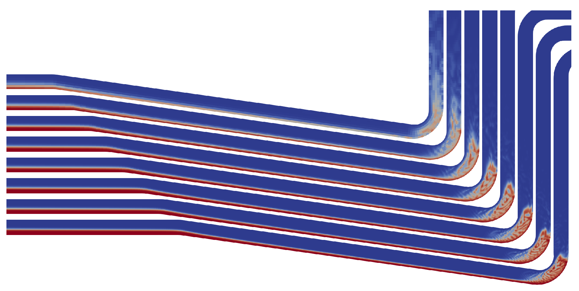
A grid independence study for the geometry has also been performed using 1st order upwind spatial discretization. The results for 1st order upwind are seen in Figure 6 and the results for 2nd order upwind are seen in Figure 7 for the same time step, represented as a contour plot of the water volume fraction during initial slug formation. In Figure 6, it can be seen that 1st order upwind gives a somewhat blurry prediction of the phase separation, which is not present for the simulation for 2nd order upwind in Figure 7. Because of this, it is evident that the simulation for 1st order upwind on the finest mesh is only similar to that for 2nd order upwind on the coarsest mesh. Thus, it is essential to use higher order discretization for slug flow simulations.

In Figure 7, when observing the interface boundaries of the solutions, smearing can be observed for the coarsest meshes due to their resolutions.

4. Results and Discussion

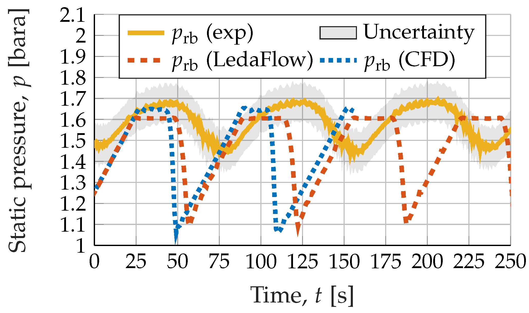
Figure 8 shows the low-point pressure amplitudes. The results of the numerical models show good correlation in terms of both pressure levels and propagation, while the experimental data shows less pressure drop during a cycle.

The difference in low-point pressure ranges is explainable by the extent the riser is emptied during blowout. Both numerical models predict that the riser is emptied during blowout. This explains the drop to atmospheric pressure as there is essentially no water column to add hydrostatic pressure. When physically observing the experiment execution, the air is evacuated from the riser through smaller Taylor bubbles flowing through a water column, adding a hydrostatic pressure component.

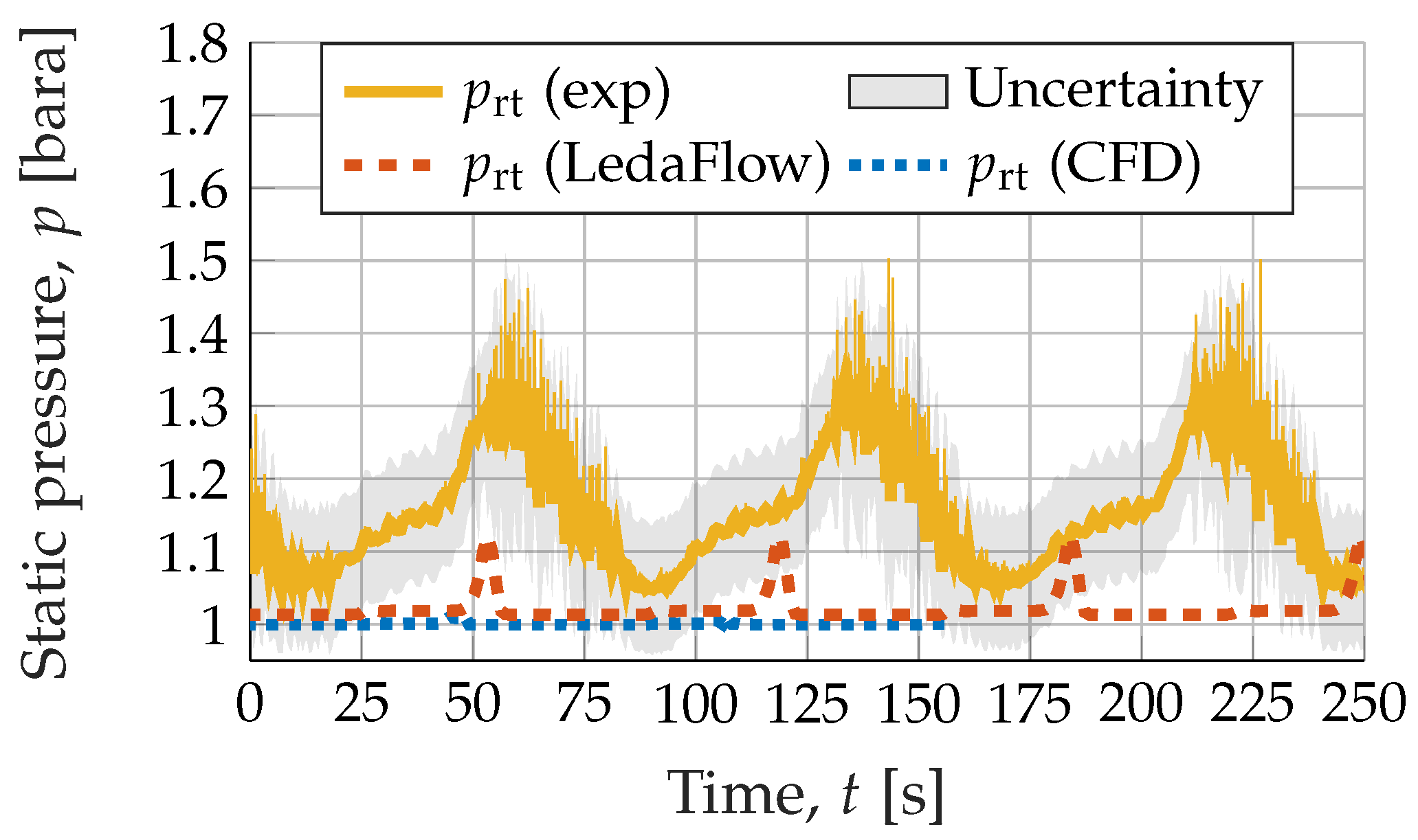
Figure 9 compares the topside pressures. By observing the plot, it is evident that the experimental pressure data is above atmospheric during the entire sampling period, which none of the numerical simulation models could reproduce.

Numerical models predict atmospheric pressure levels besides during the blowout phase, where a small pressure peak is observed, for example, at 50 s. The peak in the CFD results are barely observable from the plot, while the peak of 1D transient model is clearly distinguishable. The higher peak pressure of the LedaFlow model, compared to the CFD model, is caused by the implementation of the topside valve in the LedaFlow model, which has not been accounted for in the CFD model.

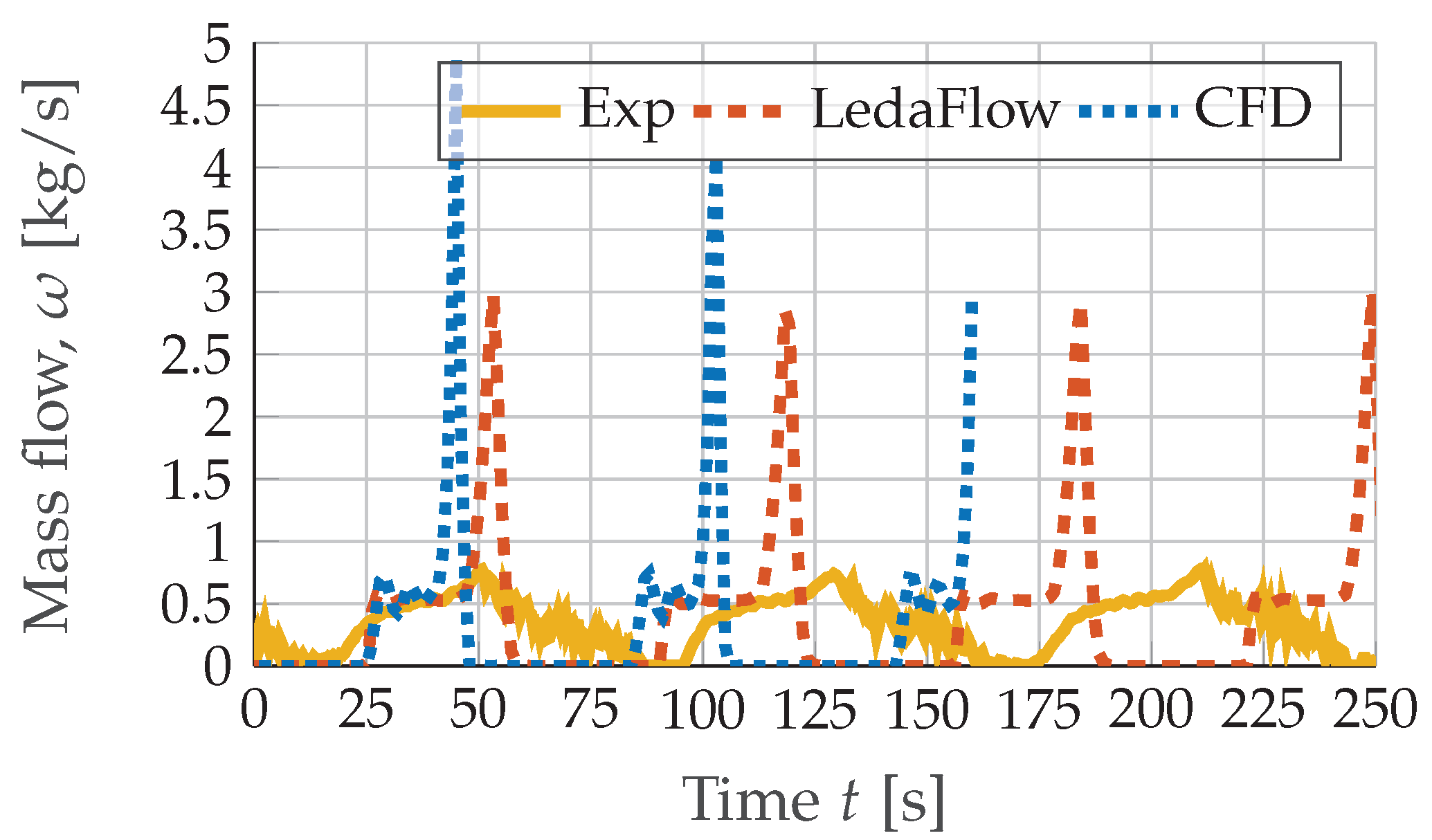
Figure 10 compares the topside mass flows. The experimental mass flow fluctuates in the range of 0–0.5 kg/s. Observing the numerical results, the mass flows are within this range, except for momentary peaks at levels of around 3 and 5 kg/s for LedaFlow and CFD, respectively. These peaks represent the blowout phase, followed by a slug formation phase where the mass flow rates reduce to approximately 0 kg/s. This is due to pure air flow at the topside position during slug formation. During liquid production, the mass flow increases to around 0.5 kg/s. These cyclic phases are clearly separated in the numerical data.

It is harder to indicate the cycle phase occurrences in the experimental data. At the liquid production phase, observable at around 75 s, numerical and experimental data shows good correlation. The blowout, fallback and slug formation phases are harder to distinguish. A small peak can be observed at 210 s, indicating a blowout, after which the mass flow decreases slowly while fluctuating, which might indicate two-phase flow topside during the remaining cycle phases. This is supported by physical observations of the experiment execution, where only the top of the riser is emptied of water, while air is evacuated from the riser afterwards through Taylor bubbles.

The high mass flow peaks of the numerical models are believed to be evidence of a more severe blowout predicted by the models compared to experimental data. This also explains the slower decrease of mass flow in the experimental data.

The inability to predict the experimentally observed blowout using the numerical models is puzzling. It is believed that the specification of the outlet pressure is the main cause of this disagreement. The outlet is specified to be at atmospheric pressure, which is justifiable, as the downstream separator is vented to the atmosphere. From observing the resulting pressure amplitudes of the model, this boundary condition does not seem to capture the damping possessed by the physical system in the current models. Also, the outlet boundary conditions might be cause of the difference in topside pressure when comparing model data to experimental.

Figure 8, Figure 9 and Figure 10 indicate a difference in slug periods which is quantified through FFT analysis of the low-point pressure data. Normalized FFT plots are presented in Figure 11 and a significant difference between the data sets is evident. The model with the best prediction of the actual slug frequency is LedaFlow, which predicts a period of 66 s compared to 78.5 s of experimental data, while the CFD model results predicts a period of 61 s. This difference is believed to be attributable to the difference in blowout progression.

The models are compared and evaluated in

Table 4. Comparison of 1D and 3D models.

Parameter	3D CFD	1D Transient
Cell count	240,550	165
Run time	57 h 30 min	11 min
Processor use	7 cores, 3.5 GHz	Serial, 2.5 GHz
Simulated time	330 s	1000 s
Predictions:
- Pressure range	Comparable
- Mass flow rate	Comparable
- Slug frequency	22.3% deviation	15.7% deviation
- Interface prediction	Good	Poor

.

The LedaFlow and CFD models perform similarly in predicting the pressure ranges and mass flow rate. For the slug period, the LedaFlow model performs slightly better than the CFD model when comparing to experimental data. The advantage of the CFD model is found to be the ability to predict phase interfaces as shown in Figure 12 for a Taylor bubble.

The runtime of LedaFlow is 1‰ that of the CFD model to simulate 330 s, where LedaFlow is run on a single core 2.5 GHz laptop and the CFD model is decomposed to utilize 7 cores on a 3.5 GHz workstation. Thus, the choice of simulation model strongly depends on the desired accuracy of the interfaces and the available time, as current models perform comparable for cycle prediction in terms of pressure levels and cycle frequency.

5. Conclusions

During this study, numerical models have been developed for predicting the flow features of a water-air flow through an experimental riser pipeline setup under operating conditions producing riser-induced slug flow. A 3D CFD model was developed based on the VOF model using RANS with the realizable k-$\epsilon$ turbulence model. The model was developed within the OpenFOAM v6 framework. In addition, a 1D transient model was developed in the commercial software LedaFlow to compare options for numerical simulation of the case.

Based on the case study’s results from the laboratory testing facility, where the models’ accuracy and computational time have been quantified and presented, the following can be concluded:

• Both commercial 1D and 3D CFD modeling can be used to simulate riser-induced slugs if the main focus is slug progression and period.
• Both developed models predicted maximum pressure levels close to experimental.
• The developed models predicted slug periods of 61 s and 66 s, while the experimental was found to be 78 s.
• The performance of the 1D and 3D models are comparable in terms of predicting pressure levels and slug frequencies.
• The 1D model is far less computationally intensive compared to 3D CFD.
• 3D CFD modeling proves superior to 1D codes in resolving phase interfaces.
• Model accuracy is expected to be further improvable by revising boundary conditions to better capture the natural damping of the physical system.
• If the selected key evaluation criteria is slug amplitude and frequency (such as for most anti-slug control schemes) both LedaFlow and 3D CFD can be used, while a focus on phase interfaces demands 3D CFD modeling.