Computational Methods for Modelling and Optimization of Flow Control Devices

 ,
,  , ,
, , 
Abstract

1. Introduction
2. Materials and Methods
2.1. Cell-Set Model
2.2. Numerical Setup
2.2.1. Setup for Cell-Set Validation (2D)
2.2.2. Setup for Optimum GF Length Calculation (2D)
2.2.3. Setup for Optimum GF Combined with a VG (3D)
2.3. jBAY Model
3. Results
3.1. Cell-Set Performance
3.2. Calculation of the Optimum GF Lenghts
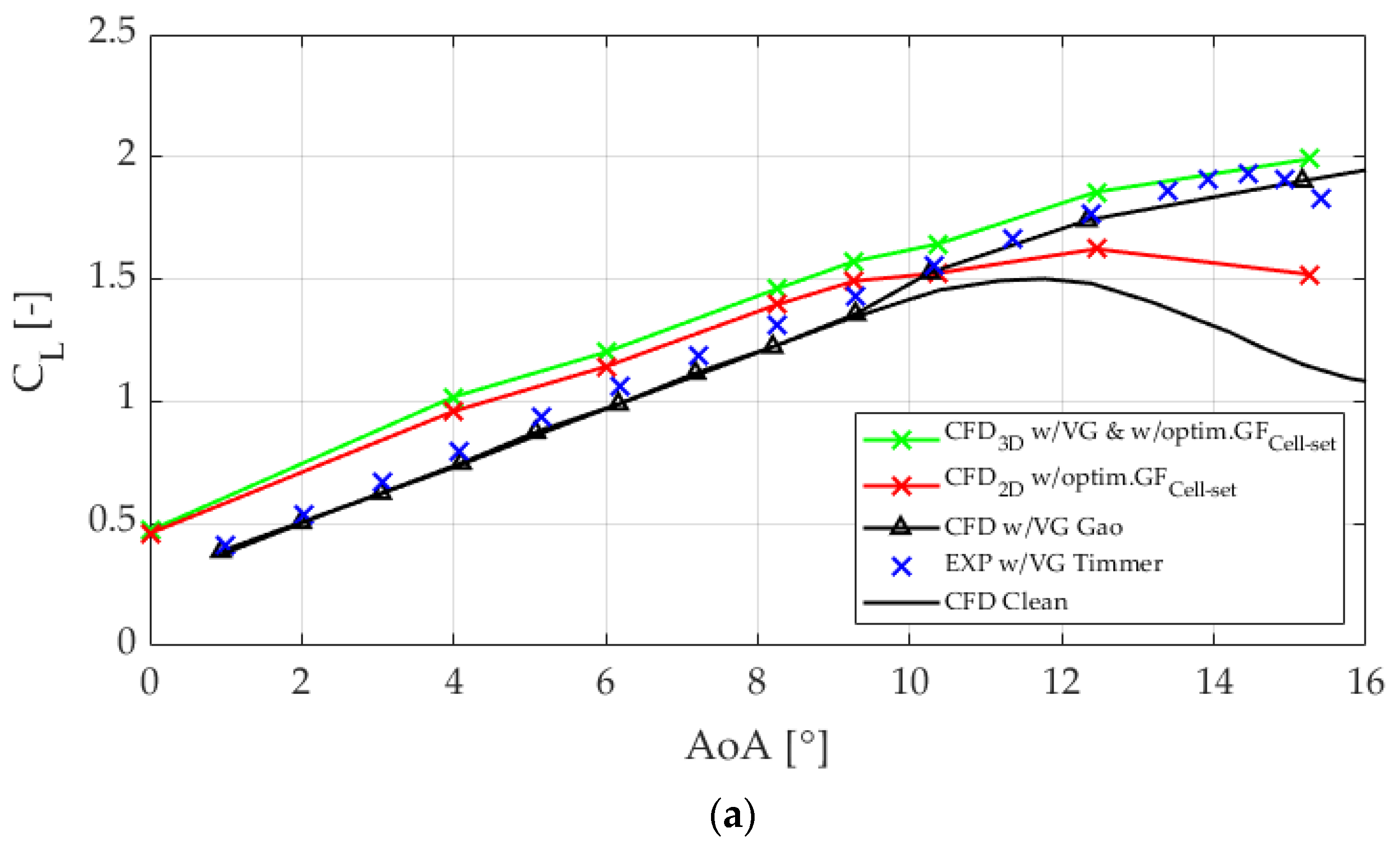
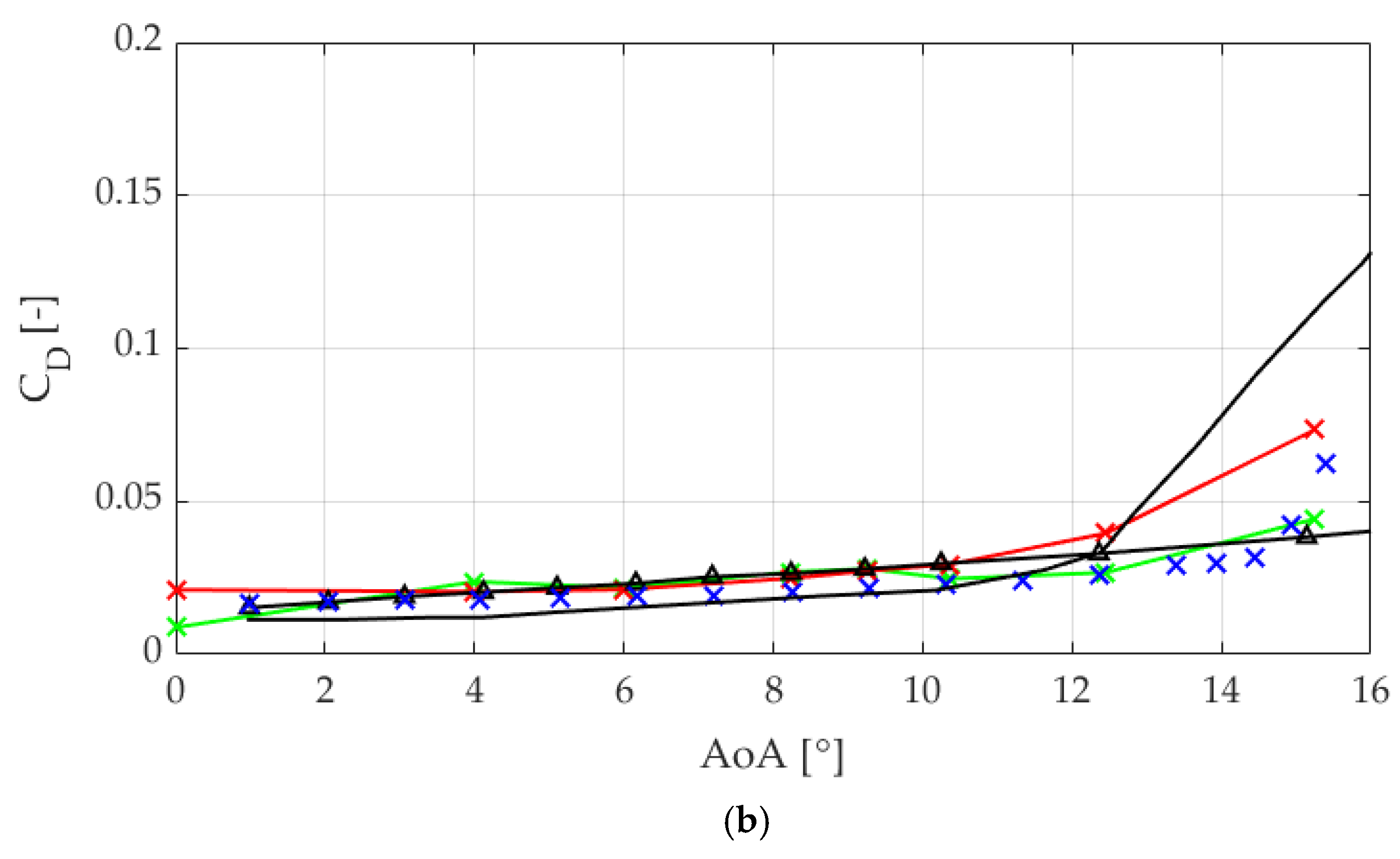
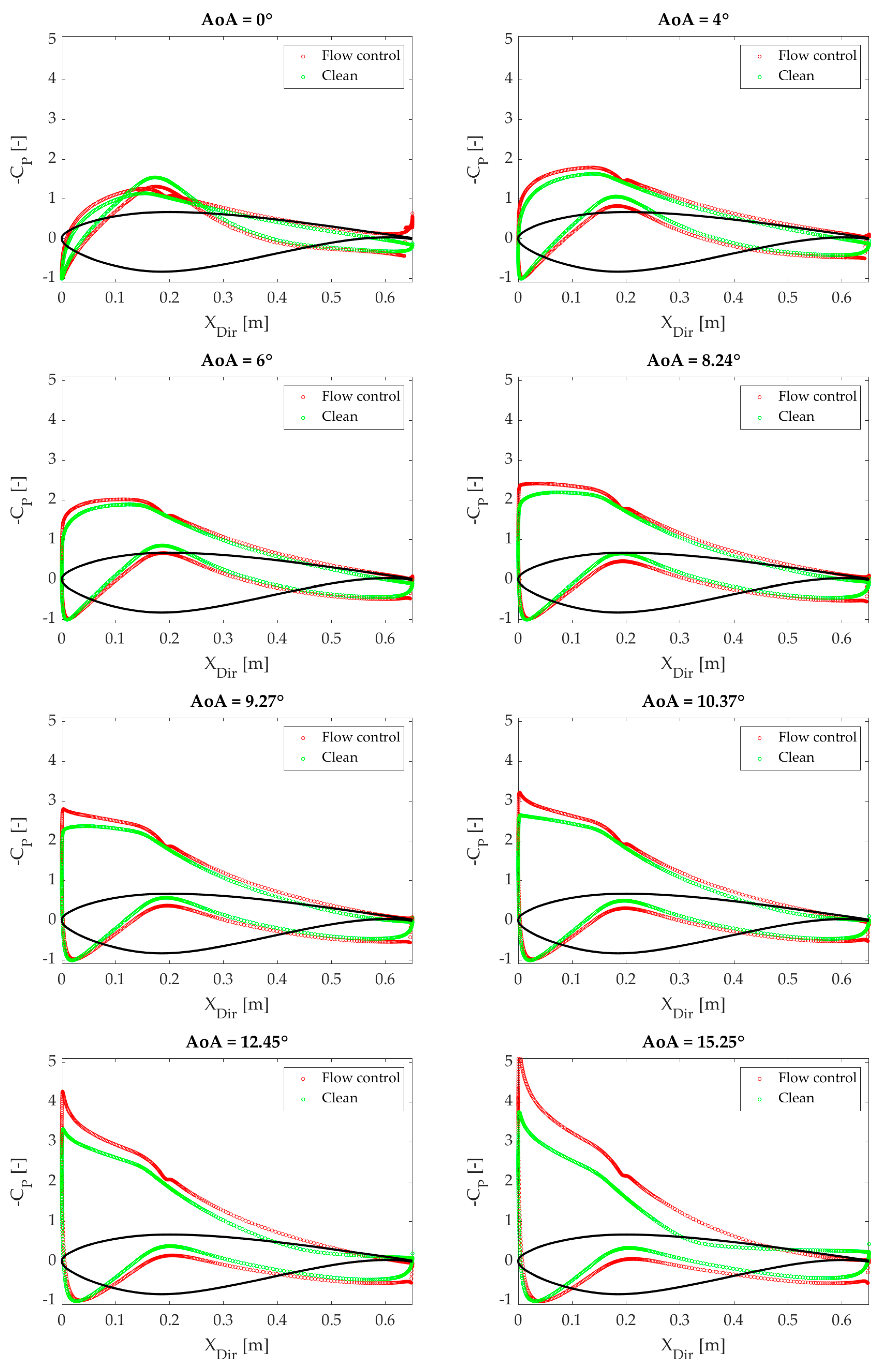
3.3. Application of the Optimum GFs
4. Conclusions
Author Contributions
Funding
Acknowledgments
Conflicts of Interest
Nomenclature
| Definition | |
| CFD | Computational fluid dynamics |
| GF | Gurney Flap |
| VG | Vortex generator |
| RANS | Reynolds-averaged Navier–Stokes |
| SST | Shear stress transport |
| Local density (kg/m3) | |
| Dynamic viscosity (Pa∙s) | |
| AoA | Angle of attack (deg) |
| c | Airfoil chord length (m) |
| hGF | Gurney flap length (% of c) |
| Relative error for each case (%) | |
| Average relative error for each hGF (%) | |
| Global relative error (%) | |
| CD | Drag coefficient |
| CL | Lift coefficient |
| CP | Pressure coefficient |
| Re | Reynolds number |
| Free stream velocity (m/s) | |
| POD | Proper orthogonal decomposition |
Appendix A

References
- Chaviaropoulos, P. Economic Aspects of Wind Turbine Aerodynamics. In Handbook of Wind Energy Aerodynamics; Springer Science and Business Media LLC: Berlin/Heidelberg, Germany, 2020; pp. 1–30. [Google Scholar]
- Pechlivanoglou, G.; Nayeri, C.; Paschereit, C. Performance Optimization of Wind Turbine Rotors with Active Flow Control (Part 1). Mech. Eng. 2012, 134, 51. [Google Scholar] [CrossRef][Green Version]
- Pechlivanoglou, G.; Nayeri, C.; Paschereit, C. Performance Optimization of Wind Turbine Rotors with Active Flow Control (Part 2). Mech. Eng. 2012, 134, 55. [Google Scholar] [CrossRef][Green Version]
- Miller, G.E. Comparative Performance Tests on the Mod-2, 2.5-mW Wind Turbine with and without Vortex Generators; Boeing Aerospace Company: Seattle, WA, USA, 1995. Available online: https://ntrs.nasa.gov/archive/nasa/casi.ntrs.nasa.gov/19950021557.pdf (accessed on 3 February 2020).
- Iradi, I.A.; Gamiz, U.F.; Saiz, J.S.; Guerrero, E.Z. State of The Art of Active and Passive Flow Control Devices for Wind Turbines. DYNA Ing. E Ind. 2016, 91, 512–516. [Google Scholar] [CrossRef]
- Aramendia, I.; Fernandez-Gamiz, U.; Ramos-Hernanz, J.; Sancho, J.; Lopez-Guede, J.M.; Zulueta, E. Flow Control Devices for Wind Turbines. In Lecture Notes in Energy; Springer Science and Business Media LLC: Berlin/Heidelberg, Germany, 2017; Volume 37, pp. 629–655. [Google Scholar]
- Hansen, M.O.L.; Madsen, H.A. Review Paper on Wind Turbine Aerodynamics. J. Fluids Eng. 2011, 133, 114001. [Google Scholar] [CrossRef]
- Velte, C.; Hansen, M.O.L. Investigation of flow behind vortex generators by stereo particle image velocimetry on a thick airfoil near stall. Wind. Energy 2012, 16, 775–785. [Google Scholar] [CrossRef]
- Godard, G.; Stanislas, M. Control of a decelerating boundary layer. Part 1: Optimization of passive vortex generators. Aerosp. Sci. Technol. 2006, 10, 181–191. [Google Scholar] [CrossRef]
- Gutierrez-Amo, R.; Fernandez-Gamiz, U.; Errasti, I.; Zulueta, E. Computational Modelling of Three Different Sub-Boundary Layer Vortex Generators on a Flat Plate. Energies 2018, 11, 3107. [Google Scholar] [CrossRef]
- Bender, E.E.; Anderson, B.H.; Yagle, P.J. Vortex Generator Modelling for Navier–Stokes Codes. In Proceedings of the 3rd ASMEJSME Fluids Engineering Conference, San Francisco, CA, USA, 18–23 July 1999. [Google Scholar]
- Fernandez-Gamiz, U.; Velte, C.; Réthoré, P.-E.; Sørensen, N.N.; Egusquiza, E. Testing of self-similarity and helical symmetry in vortex generator flow simulations. Wind. Energy 2015, 19, 1043–1052. [Google Scholar] [CrossRef]
- Chillon, S.; Uriarte-Uriarte, A.; Aramendia, I.; Martínez-Filgueira, P.; Fernandez-Gamiz, U.; Ibarra-Udaeta, I. jBAY Modeling of Vane-Type Vortex Generators and Study on Airfoil Aerodynamic Performance. Energies 2020, 13, 2423. [Google Scholar] [CrossRef]
- Fernandez-Gamiz, U.; Errasti, I.; Gutierrez-Amo, R.; Boyano, A.; Barambones, O. Computational Modelling of Rectangular Sub-Boundary Layer Vortex Generators. Appl. Sci. 2018, 8, 138. [Google Scholar] [CrossRef]
- Kumar, P.M.; Samad, A. Introducing Gurney flap to Wells turbine blade and performance analysis with OpenFOAM. Ocean Eng. 2019, 187, 106212. [Google Scholar] [CrossRef]
- Alber, J.; Pechlivanoglou, G.; Paschereit, C.O.; Twele, J.; Weinzierl, G. Parametric Investigation of Gurney Flaps for the Use on Wind Turbine Blades. In Proceedings of the Volume 1: Aircraft Engine; Fans and Blowers; Marine; Honors and Awards; ASME International: Charlotte, NC, USA, 2017; Volume 9, p. 009-49-015. [Google Scholar]
- Fernandez-Gamiz, U.; Mármol, M.M.G.; Rebollo, T.C. Computational Modeling of Gurney Flaps and Microtabs by POD Method. Energies 2018, 11, 2091. [Google Scholar] [CrossRef]
- Jonkman, J.; Butterfield, S.; Musial, W.; Scott, G. Definition of a 5-MW Reference Wind Turbine for Offshore System Development; Technical Report NREL/TP-500-38060; National Renewable Energy Laboratory: Golden, CO, USA, 2009.
- Siemens Star CCM+ Version 14.02.012. Available online: https://www.plm.automation.siemens.com/global/en/ (accessed on 3 February 2020).
- Menter, F.R. Two-equation eddy-viscosity turbulence models for engineering applications. AIAA J. 1994, 32, 1598–1605. [Google Scholar] [CrossRef]
- Sieros, G.; Jost, E.; Lutz, T.; Papadakis, G.; Voutsinas, S.; Barakos, G.; Colonia, S.; Baldacchino, D.; Baptista, C.; Ferreira, C. CFD code comparison for 2D airfoil flows. J. Physics Conf. Ser. 2016, 753, 082019. [Google Scholar] [CrossRef]
- Aramendia, I.; Fernandez-Gamiz, U.; Zulueta, E.; Saenz-Aguirre, A.; Teso-Fz-Betoño, D. Parametric Study of a Gurney Flap Implementation in a DU91W (2) 250 Airfoil. Energies 2019, 12, 294. [Google Scholar] [CrossRef]
- Timmer, W.A.; van Rooij, R.P.J.O.M. Summary of the Delft University Wind Turbine Dedicated Airfoils. J. Sol. Energy Eng. 2003, 125, 488–496. [Google Scholar] [CrossRef]
- Gao, L.; Zhang, H.; Liu, Y.; Han, S. Effects of vortex generators on a blunt trailing-edge airfoil for wind turbines. Renew. Energy 2015, 76, 303–311. [Google Scholar] [CrossRef]
- Jirasek, A. Vortex-Generator Model and Its Application to Flow Control. J. Aircr. 2005, 42, 1486–1491. [Google Scholar] [CrossRef]
- Fernandez, U.; Réthoré, P.-E.; Sørensen, N.N.; Velte, C.M.; Zahle, F.; Egusquiza, E. Comparison of four different models of vortex generators. In Proceedings of the EWEA 2012—European Wind Energy Conference & Exhibition, Copenhagen, Denmark, 16–19 March 2012. [Google Scholar]
- Errasti, I.; Gamiz, U.F.; Martínez-Filgueira, P.; Blanco, J. Source Term Modelling of Vane-Type Vortex Generators under Adverse Pressure Gradient in OpenFOAM. Energies 2019, 12, 605. [Google Scholar] [CrossRef]
- Zhao, Z.; Li, T.; Wang, T.; Liu, X.; Zheng, Y. Numerical investigation on wind turbine vortex generators employing transition models. J. Renew. Sustain. Energy 2015, 7, 063124. [Google Scholar] [CrossRef]
- Li, X.; Liu, W.; Zhang, T.; Wang, P.; Wang, X. Analysis of the Effect of Vortex Generator Spacing on Boundary Layer Flow Separation Control. Appl. Sci. 2019, 9, 5495. [Google Scholar] [CrossRef]


| hGF (% of c) | ||||||||
|---|---|---|---|---|---|---|---|---|
| AoA [°] | 0.25 | 0.5 | 0.75 | 1 | 1.25 | 1.5 | 1.75 | 2 |
| 0 | 0.478 | 1.391 | 0.031 | 0.581 | 1.816 | 0.134 | 1.566 | 0.082 |
| 1 | 0.325 | 1.310 | 0.159 | 0.913 | 2.990 | 0.253 | 2.248 | 0.422 |
| 2 | 0.224 | 2.295 | 1.561 | 1.082 | 3.520 | 0.392 | 2.618 | 0.629 |
| 3 | 0.120 | 1.293 | 0.216 | 1.082 | 3.715 | 0.295 | 2.753 | 0.687 |
| 4 | 0.680 | 1.885 | 0.106 | 1.053 | 3.635 | 0.166 | 2.664 | 0.612 |
| 5 | 0.527 | 1.855 | 0.016 | 0.890 | 0.118 | 0.095 | 2.425 | 0.429 |
| 0.392 | 1.672 | 0.348 | 0.933 | 2.632 | 0.222 | 2.379 | 0.477 | |
| hGF (% of c) | |||||||||
|---|---|---|---|---|---|---|---|---|---|
| AoA [°] | No GF | 0.25 | 0.5 | 0.75 | 1 | 1.25 | 1.5 | 1.75 | 2 |
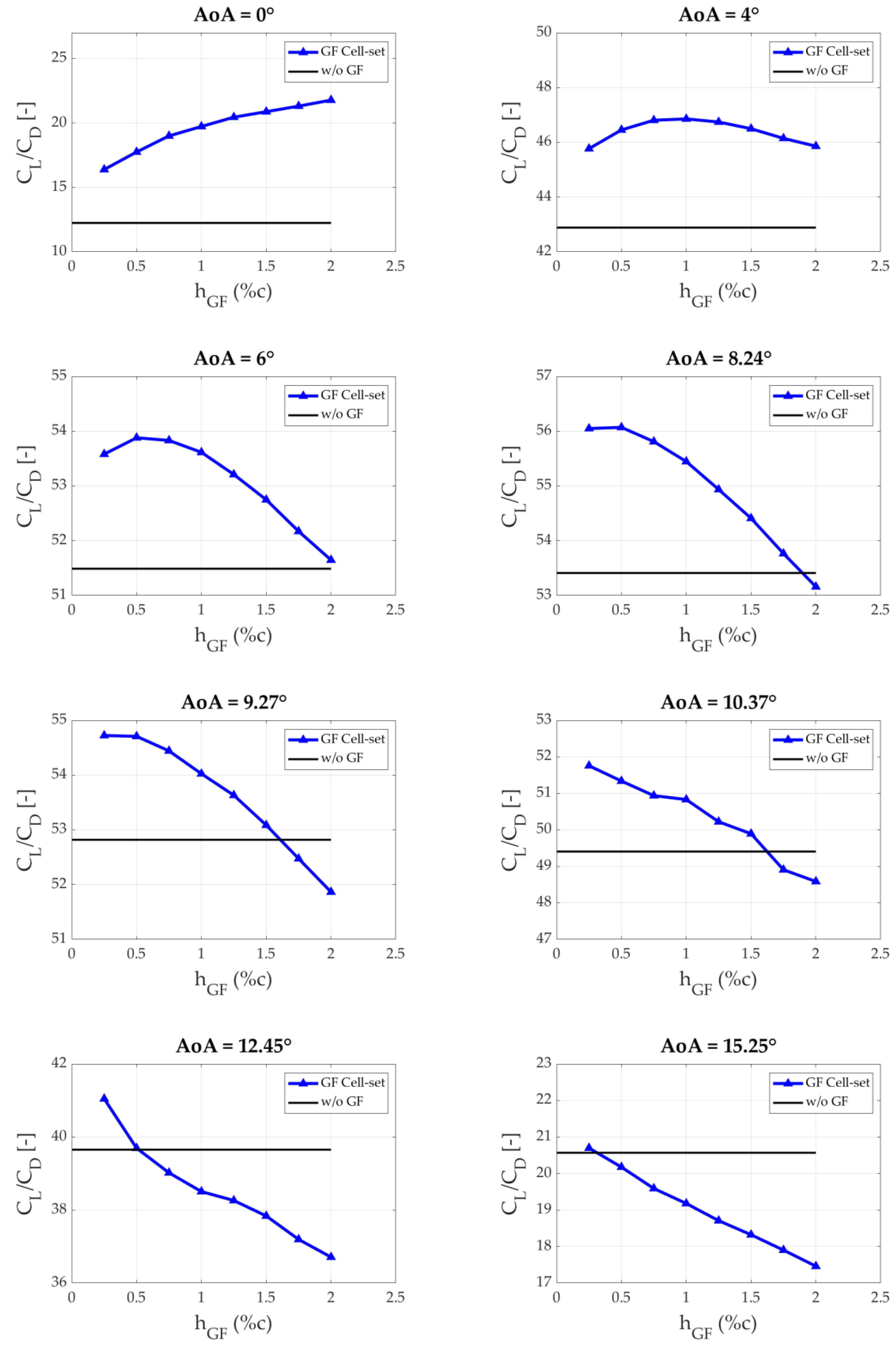
| 0 | 12.24 | 16.39 | 17.75 | 18.99 | 19.73 | 20.45 | 20.87 | 21.31 | 21.77 |
| 4 | 42.89 | 45.77 | 46.45 | 46.80 | 46.85 | 46.74 | 46.49 | 46.14 | 45.86 |
| 6 | 51.49 | 53.58 | 53.88 | 53.83 | 53.61 | 53.21 | 52.75 | 52.17 | 51.65 |
| 8.24 | 53.41 | 56.05 | 56.07 | 55.81 | 55.45 | 54.93 | 54.41 | 53.77 | 53.16 |
| 9.27 | 52.82 | 54.70 | 54.71 | 54.44 | 54.02 | 53.63 | 53.09 | 52.47 | 51.86 |
| 10.37 | 49.41 | 51.75 | 51.34 | 50.94 | 50.83 | 50.22 | 49.89 | 48.91 | 48.58 |
| 12.45 | 39.65 | 41.05 | 39.69 | 39.02 | 38.50 | 38.26 | 37.84 | 37.19 | 36.71 |
| 15.25 | 20.57 | 20.70 | 20.17 | 19.59 | 19.18 | 18.71 | 18.32 | 17.90 | 17.46 |
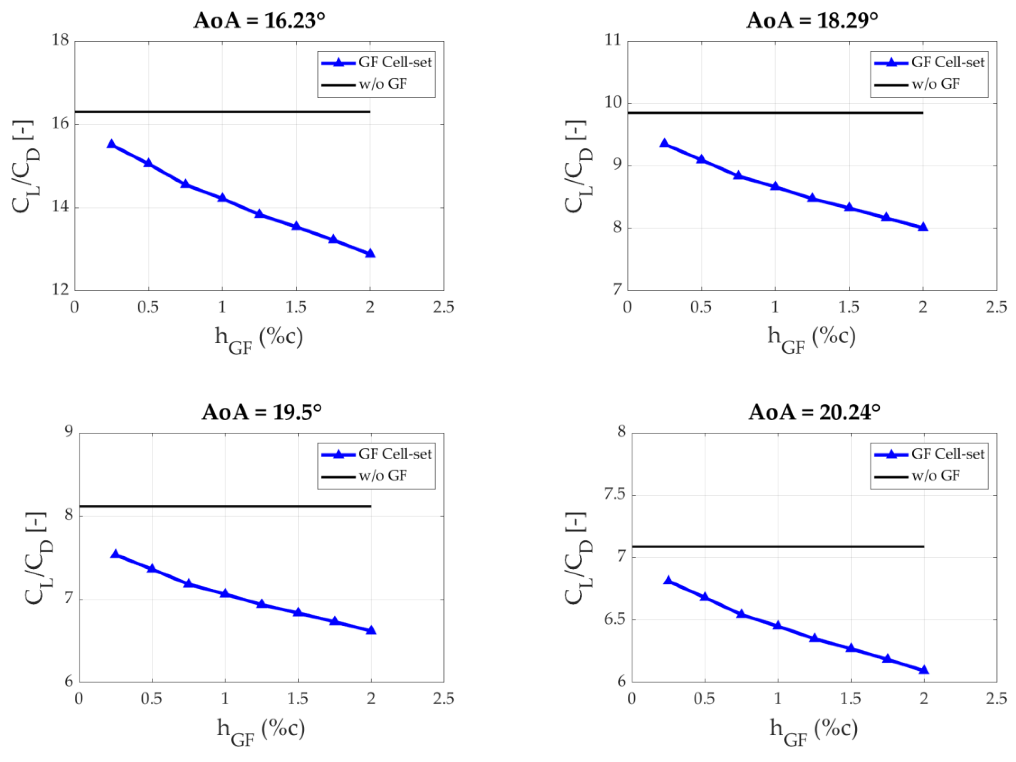
| 16.23 | 16.30 | 15.50 | 15.05 | 14.55 | 14.21 | 13.83 | 13.53 | 13.22 | 12.88 |
| 18.29 | 9.85 | 9.35 | 9.09 | 8.84 | 8.66 | 8.47 | 8.33 | 8.17 | 8.01 |
| 19.5 | 8.12 | 7.53 | 7.36 | 7.18 | 7.06 | 6.93 | 6.83 | 6.73 | 6.62 |
| 20.24 | 7.09 | 6.81 | 6.68 | 6.54 | 6.45 | 6.35 | 6.27 | 6.18 | 6.09 |
| AoA [°] | max. CL/CD [-] | Opt. hGF (% of c) |
|---|---|---|
| 0 | 21.77 | 2 |
| 4 | 46.85 | 1 |
| 6 | 53.88 | 0.5 |
| 8.24 | 56.07 | 0.5 |
| 9.27 | 54.71 | 0.5 |
| 10.37 | 51.75 | 0.25 |
| 12.45 | 41.05 | 0.25 |
| 15.25 | 20.70 | 0.25 |
© 2020 by the authors. Licensee MDPI, Basel, Switzerland. This article is an open access article distributed under the terms and conditions of the Creative Commons Attribution (CC BY) license (http://creativecommons.org/licenses/by/4.0/).
Share and Cite
Ballesteros-Coll, A.; Fernandez-Gamiz, U.; Aramendia, I.; Zulueta, E.; Lopez-Guede, J.M. Computational Methods for Modelling and Optimization of Flow Control Devices. Energies 2020, 13, 3710. https://doi.org/10.3390/en13143710
Ballesteros-Coll A, Fernandez-Gamiz U, Aramendia I, Zulueta E, Lopez-Guede JM. Computational Methods for Modelling and Optimization of Flow Control Devices. Energies. 2020; 13(14):3710. https://doi.org/10.3390/en13143710
Chicago/Turabian StyleBallesteros-Coll, Alejandro, Unai Fernandez-Gamiz, Iñigo Aramendia, Ekaitz Zulueta, and Jose Manuel Lopez-Guede. 2020. "Computational Methods for Modelling and Optimization of Flow Control Devices" Energies 13, no. 14: 3710. https://doi.org/10.3390/en13143710
APA StyleBallesteros-Coll, A., Fernandez-Gamiz, U., Aramendia, I., Zulueta, E., & Lopez-Guede, J. M. (2020). Computational Methods for Modelling and Optimization of Flow Control Devices. Energies, 13(14), 3710. https://doi.org/10.3390/en13143710