Article

Dynamics of Connectedness in Clean Energy Stocks

by
Fernanda Fuentes
1,† and
Rodrigo Herrera
2,*,†
1
DSc Program on Complex Engineering Systems, Institute of Mathematics and Physics, University of Talca, Talca 3460000, Chile
2
Faculty of Business and Economics, University of Talca, Talca 3460000, Chile
*
Author to whom correspondence should be addressed.
These authors contributed equally to this work.
Energies 2020, 13(14), 3705; https://doi.org/10.3390/en13143705
Submission received: 3 June 2020 / Revised: 8 July 2020 / Accepted: 16 July 2020 / Published: 18 July 2020
(This article belongs to the Section C: Energy Economics and Policy)

Abstract

:
This paper examines the dynamics of connectedness among the realized volatility indices of 16 clean energy stocks belonging to the SPGCE and the implied volatility indices of two important stock markets—the S&P 500 and the STOXX50—and two commodities markets—the crude oil and gold markets. The empirical results show a unidirectional connectedness from the implied volatility indices to the clean energy stocks. Our analysis further reveals similar volatility connectedness behaviors among companies in the same energy production subsector. However, there exists heterogeneous behavior between different energy production subsectors over time. Further, we identify pairwise directional connectedness clusters among related companies, indicating that there are few possibilities for portfolio diversification within the energy production subsectors. Finally, through an impulse–response analysis, we confirm that the expectation of future market volatility of the S&P 500 index and the gold price plays a leading role in volatility connectedness with clean energy stocks.

1. Introduction

Global economic development is intricately tied to the supply and demand of energy. At present, the largest source of energy is fossil fuels, the use of which accounts for 87% of global carbon dioxide CO2 emissions [1,2,3]. Over the last few years, national governments have taken a variety of actions to reduce greenhouse gas emissions and to help make renewable energy competitive with conventional energy sources [4,5,6]. Within these new stock markets, clean energy stocks have attracted the attention of both investors and energy policy analysts, who are interested in understanding the behavior of these stocks and determining whether these new investment opportunities hold promise [7,8,9].
The literature on clean energy stocks is scarce, and the majority of research has used global clean energy indices to represent the behavior of these markets. The S&P Global Clean Energy Index (SPGCE), WilderHill Clean Energy Index (ECO), and WilderHill New Energy Global Innovation Index (NEX) are the main indices used (see Table 1). Nevertheless, conducting analyses using only global clean energy indices—thereby excluding company-level information—can lead to flaws in the conclusions of studies [10]. Commonly, the relationships between clean energy indices and other financial markets have been studied using multivariate volatility models [7,11,12,13] and multivariate copulas models [1,14,15]. While both of these methodologies provide researchers with useful information in different contexts, neither provides any insights related to directional connectedness.
Our study extends the current literature in several ways: (i) We analyze the volatility connectedness among individual clean energy stocks from distinct subsectors of production; (ii) we include implied volatility indices to investigate the expectations of financial markets regarding individual clean energy stocks; (iii) we determine whether the clean energy stocks are more affected by expectations from financial markets (i.e., the USA or Europe) or commodity markets (i.e., oil or gold); (iv) we analyze volatility connectedness to determine the magnitude and direction of volatility spillovers and observe the dynamics of connectedness between markets; and (v) we complement our results with an impulse–response analysis to determine the impact of a shock in the implied volatility indices on the volatility of clean energy stocks.
The motivation to include implied volatility indices from commodity and global stock markets is because these two markets have become important economic and financial indicators representing market consensus on the expected future uncertainty [15,16,17]. Therefore, the estimated volatility connectedness of commodity and stock markets with the realized volatility of the clean energy stocks is informative of the different nature of risk transfer associated with trading activity and cross-market sentiments of the market participants. In particular, energy stock prices have different effects across industries or sectoral stock markets; for instance, energy-intensive firms should be more influenced by large oil volatility shocks, indicating a negative relationship between increasing oil prices and stock prices [18,19]. As oil prices rise, economic agents are motivated to seek alternative energy sources, such as clean energy markets. On the other hand, technology stocks are susceptible to the business cycle; influencing also clean energy firms that, at the same time, depend on inputs from technology companies [20,21]. Hence, clean energy stocks and technology stocks are closely related to the business cycle. Thus, the results of this research provide useful information to risk managers looking for diversification strategies using derivatives on an investment portfolio during periods of financial turmoil.
Our analysis includes the realized range-based volatility of 16 individual clean energy stocks, all belonging to the SPGCE index. These companies include solar, wind, and hydroelectric energy producers located in countries such as the United States, Canada, Brazil, Denmark, and China. Our study provides a more detailed vision of the behavior of clean energy stocks by using the information from four implied volatility indices to define the expectations for future volatilities in clean energy stocks. The following indices have been identified in the existing literature as having important links with clean and conventional energy stocks: CBOE Gold ETF Volatility Index ( G V Z ) , CBOE Crude Oil ETF Volatility Index ( O V X ) , CBOE Volatility Index based on options of the S&P 500 index ( V I X ) , and EURO STOXX 50 Volatility Index based on EURO STOXX 50 options prices ( V S T O X X ) . The CBOE acronym refers to Chicago Board Options Exchange. The first two implied volatility indices are associated with commodities; oil is known as an inherent substitute in clean energy stocks [22,23], while gold is included for its role as an effective safe haven in the face of stressful financial situations [15,24,25]. The second two are global indices, from the United States and Europe, respectively. These indices were included due to the countries of origin of the companies. Unlike the previous literature, which examined these indices from an aggregate point of view, our research shows that, if we want to find the most efficient investment strategies, we must acknowledge that each subsector of energy production has specific characteristics. In this context, the main research questions posed are: Are the volatility prices of clean energy stocks heterogeneous across the different clean energy production subsectors? And how clean energy stock prices, of different production subsectors, relate to the changes in prices of the main financial and commodity markets? This information is relevant to investors and energy policy analysts who are interested in understanding the behavior of clean energy stocks, in order to determine whether these new investment opportunities are attractive [7,8,9]
To estimate the directional volatility spillover measures between the realized volatility of clean energy stocks and the implied volatility indices, we use the Diebold–Yilmaz connectedness methodology (see [26]). This methodology provides a useful framework for estimating directional connectedness between individual series and offers important summary measures of network connectedness. We chose this methodology for several reasons. First, this approach can be easily implemented by means of a vector autoregression model through forecast error variance decomposition. More importantly, this framework quantifies both the direction and strength of dynamic connectedness among different variables. Second, it allows the use of different time horizons, facilitating selection suitable for each context. Third, it overcomes the dimensionality problem that arises from an increase in the number of variables included in the analysis.
Our results reveal that connectedness is unidirectional, marked by the strong flow of information from the implied volatility indices toward the clean energy stocks, where the future volatility expectations of V I X and G V Z play fundamental roles. By examining the dynamics of the volatility connectedness, it is possible to identify cross-sectional patterns among companies from the same subsector of production. As a result, we can identify a heterogeneous relationship between subsectors of clean energy production (i.e., solar, wind, hydroelectric, geothermal, fuel cell, and mixed) and the implied volatility indices. Finally, an impulse–response analysis allows us to confirm the results of directional connectedness, highlighting the impact of shocks in V I X and G V Z on the realized volatility of the clean energy stocks. Furthermore, using this analysis method, we can once again observe cross-sectional patterns among the connectedness measures of distinct subsectors of clean energy production.
The remainder of this paper is organized as follows. Section 2 presents a review of the literature. In Section 3, we provide a description of the data. Then, in Section 4, we present the methodology and, in Section 5, we analyze the empirical results of this study. Finally, we offer some concluding remarks in Section 6.

2. Literature Review
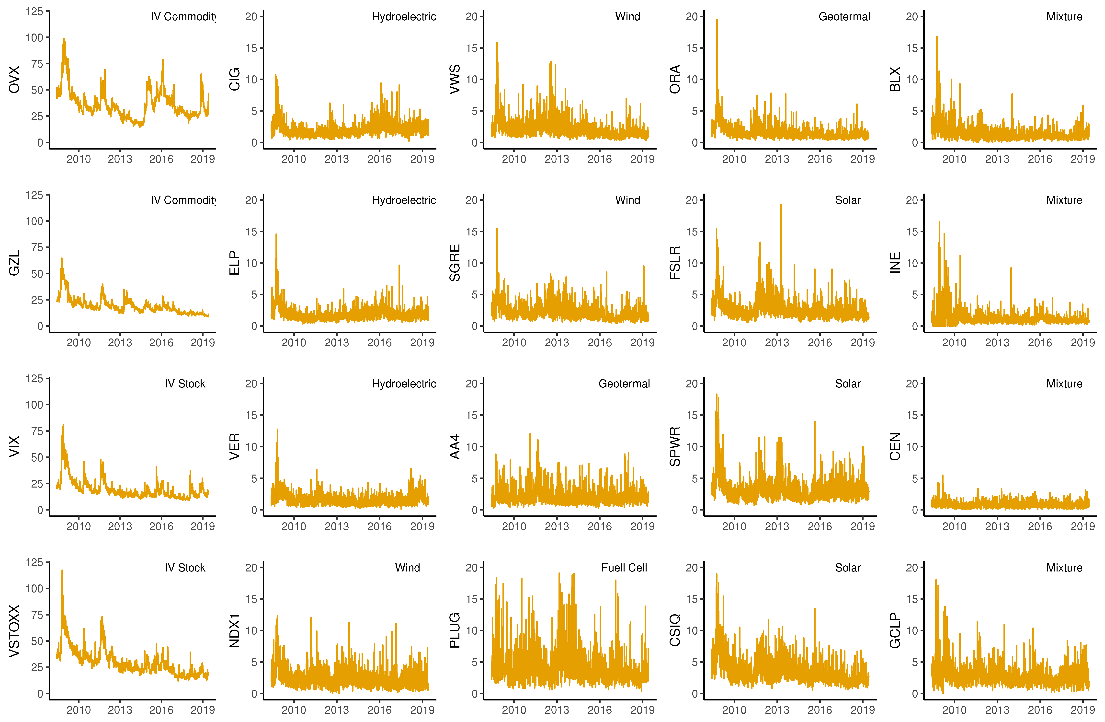
A growing interest in sustainable development has led to increasing investor awareness of clean energy stocks and expanding research on the relationship between those stocks and other financial markets. Table 1 presents a detailed overview of the literature on clean energy stocks, identifying the main methodologies and indices used in each study.
The first studies on clean energy stocks used VAR models; for instance, Kumar et al. [23] used a VAR model to show that the price behavior of clean energy stocks can be explained by past movements in oil prices, stock prices of high-technology firms, and interest rates. In this study, carbon price returns are not a significant factor in stock price movements for clean energy firms. Managi and Okimoto [27] proposed a Markov Switching VAR model to examine the relationships between clean energy, oil, and technology stock prices. Their results indicated a positive relationship between these stock’s market indices, a relationship that started with a structural change in late 2007.
Another strand of literature focuses more on the interdependence of volatility than on its price returns. For example, Sadorsky [28] compared different multivariate GARCH models (BEKK, Diagonal, DCC, and CCC) to model conditional correlations and to analyze volatility spillovers between oil prices and the stock prices of clean energy and technology companies. The results indicated that the stock prices of clean energy companies were more highly correlated with technology stock prices than with oil prices. Ahmad et al. [16] used DCC, ADCC, and GO-GARCH models to examine how crude oil, US bonds, gold, VIX, OVX, and European carbon prices can be used to hedge an investment in clean energy equities. Their study shows that VIX is the best asset for protecting clean energy equities, followed by oil and gold. Dutta et al. [11], using a bivariate VAR-GARCH approach, studied the relationship between the carbon emissions market and renewable energy stock returns. They found a significant volatility linkage between the carbon emission returns and the prices of clean energy in European markets; however, this relationship did not hold for US markets. Kyritsis and Serletis [12] used VAR-GARCH-in-mean to estimate an impulse–response analysis of clean energy stock markets and technology company stocks with the different sized shocks in oil price shocks. The results suggested that there was a symmetric relationship between oil and the returns of clean energy stocks. Maghyereh et al. [13] proposed a wavelet MGARCH-DCC method to analyze the bidirectional relationships between the returns and volatilities from oil and technology to the clean energy market using multiple time horizons. Their main finding was that, over long time horizons, the returns and volatilities of oil significantly and positively affected clean energy stock markets. When considering all time horizons, there exists a bidirectional relationship between the returns and volatilities of technology and clean energy stocks. Dutta et al. [7], through a DCC-GARCH model, showed that commodity volatilities and clean energy equity prices move in opposite directions, suggesting the possibility of using implied volatility indices as an effective tool for hedging clean energy stock indices.
More recent literature has analyzed the behavior of clean energy stocks and their contemporary relationships with other markets using multivariate copula functions. Mejdoub and Ghorbel [1] used a TGARCH-Vine copula to determine how changes in oil prices affect renewable energy stock markets. Their results indicated a significant and symmetric dependence between both markets, which were coupled in the same direction. Reboredo and Ugolini [14] carried out a study based on a multivariate vine copula to characterize the dependence between different classes of energy (i.e., oil, gas, coal, and electricity) and the price of clean energy. Their analysis showed that oil and electricity were the main contributors to the dynamics of clean energy prices. Bouri et al. [15] carries out a two-stage study: First, they utilized a mixture specification copula and, then, they performed an analysis of parametric and non-parametric tail dependence measures. The objective of their study was to verify the role of gold and oil as potential safe havens for clean energy indices in times of crisis. Their results showed that both commodities were no more than weak safe-haven stocks for clean energy indices, where oil was better during extreme price movements. Reboredo [22] used TGARCH-copulas to characterize the structural dependence between oil and three international clean energy indices (ECO, SPGCE, ERIX), incorporating the indices of different production sectors as well (i.e., solar, wind, smart technologies). His results showed a symmetric tail dependence in almost all of the clean energy indices; except for the solar energy index, which was asymmetrically affected by extreme movements in oil prices.
Recent studies have used the Diebold–Yilmaz methodology (see [26]) to analyze the connectedness between clean energy stocks and other markets. Connectedness is central for risk mediation and management, thus playing a pivotal role in risk markets, credit risk, counter-party and gridlock risk, and systemic risk [29]. In this vein, Ahmad [30] determined that technology and clean energy indices are the dominant emitters of return and volatility spillovers to crude oil. Furthermore, the authors showed evidence that clean energy indices can provide a profitable hedging opportunity in combination with oil and technology indices. Ahmad and Rais [31] determined the existence of directional spillover from technologies to clean energy markets and a bidirectional dependence with global stock markets. Pham [10] identified the subsectors of production to analyze the connectedness between oil and different clean energy indices. The results showed that biofuel and energy management stocks (NASDAQ OMX Energy Management Index) were more connected with oil price, while wind, geothermal, and fuel cell stocks were among the least connected to oil price. The study asserted that disaggregating the analysis to the level of the production subsector is necessary for effectively studying the behavior of clean energy stocks.
Finally, there also exist other methodologies to analyze the dependence among clean energy markets which are not classified among the previously mentioned ones; for instance, Sadorsky [32] used an extension of the capital asset pricing model to investigate the determinants of risk in clean energy stocks. The results showed that increased oil prices have a positive impact on the financial risk of clean energy stocks. Bondia et al. [33] analyzed cointegration and causality, providing evidence that clean energy stocks are affected by technology stock prices, oil prices, and interest rates in the short term. Dutta [17] used a realized volatility model to demonstrate that clean energy stocks are highly sensitive to shocks in the OVX. Reboredo et al. [34] proposed a wavelet analysis and Granger causality test to examine co-movement and causality between oil and renewable energy indices. Their results indicated that there is a weak relationship in the short term that gradually gets stronger over the long term. Yahşi et al. [35] developed a prediction model for future carbon prices using explanatory variables. Their main findings indicated that the variable with the most influence on future carbon prices is clean energy stocks.
One important weakness in the recent literature is that most studies have used global indices to represent the general behavior of clean energy markets. To the best of our knowledge, the only studies that have shown differences in their results after identifying subsectors of production are those of Reboredo [22] and Pham [10]. In particular, Pham [10] was the first to identify that using global indices of clean energy is a weakness when attempting to capture the heterogeneity of the subsectors of clean energy production. For this reason, our study offers a more detailed understanding of the behavior of clean energy stocks at the company level, thereby differentiating clean energy companies from different subsectors of production.

3. Data Description

Volatility, as a quantitative indicator of risk or uncertainty, is one of the most important measures for describing market expectations. The connectedness of volatility is known as the “connectedness of fear,”which has become an interesting area of study [36,37]. Quantifying these effects could inform early alert systems to warn of emerging crises [11].
This study uses the daily realized volatility indices for 16 clean energy stocks belonging to the SPGCE as its time-series. To obtain the realized volatility indices, we constructed the realized range-based volatility following Garman and Klass [38]:
σ ^ i t 2 = 0.511 H i t L i t 2 0.019 C i t O i t H i t + L i t 2 O i t 2 H i t O i t L i t O i t 0.383 C i t O i t 2 ,
where H i t , L i t , O i t , and C i t are the high, low, opening, and closing prices, respectively, using the logs of stock prices i over time t.
In Table 2, we give a description of the companies, including the name, abbreviation, origin (country and year that it was founded), and the sector of production of each company. Representative in the sample are solar energy, wind energy, geothermic energy, fuel cell, and hydroelectric producers located in countries such as the United States, Canada, Brazil, Denmark, and China (The companies that operate in more than one sector of production are labeled “mixture” in Table 2). We also include four implied volatility indices: CBOE Gold ETF Volatility Index ( G V Z ) , CBOE Crude Oil ETF Volatility Index ( O V X ) , CBOE Volatility Index based on options of the S&P 500 index ( V I X ) , and EURO STOXX 50 Volatility Index based on EURO STOXX 50 options prices ( V S T O X X ) . The first two implied volatility indices are associated with commodities; oil is known as an inherent substitute in clean energy stock prices [22,23], while gold is included for its role as an effective safe haven in the face of stressful financial situations [15,24,25]. The second two are global indices, from the United States and Europe, respectively. These indices were included because of the countries of origin of the companies. All data were obtained from the Thomson Reuters Datastream, with daily observations from 3 June 2008 to 3 June 2019. Because the OVX index has been published since the middle of the year 2008, only 16 of the 30 stock indices that make up the SPGCE were used for this study, as these were the only ones with information available for the whole sample period.
Figure 1 shows the implied volatility and realized volatility indices. In most cases, we observe an increase in volatility during the 2008 subprime crisis. Among the implied volatility indices in the left column, O V X stands out as having several spikes in volatility over the full sample period. In the case of the realized volatility estimations for the clean energy stocks, they show a more stable behavior over time than those exhibited by the implied volatility indices. In particular, if we focus on the sector of production of each company, we observe similar patterns and trends for companies whose production source is the same; for instance, CIG, ELP, and VER are all hydroelectric energy companies, whose returns exhibit similar stylized facts.
Table 3 provides a wide descriptive statistics for both types of volatilities. The implied volatility indices show higher medians and standard deviations than those observed in the realized volatility indices of the clean energy stocks. Furthermore, all of the volatility indices have positive asymmetry and show a leptokurtic distribution. These results were confirmed by the Jarque–Bera test, which rejected the normality of the observations. The Box–Pierce test statistic, estimated with 10 lags, showed evidence of persistence. The Phillips–Perron test was used to examine the stationarity of the price volatilities. The results showed that all volatilities were stationary at the 0.05 significance level.

4. Methodology

To quantify the causal relationship between the realized volatility of clean energy stocks and the implied volatility of the global stock markets and commodity indices, we applied the Diebold–Yilmaz connectedness methodology [26]. This approach is based on a forecast error variance decomposition, employing a generalized VAR framework [39] of order p,
y t = i = 1 p Φ y t i + ε t ,
where y t is an M-dimensional vector of endogenous variables containing the set of realized volatility and implied volatility indices, ε t N ( 0 , Σ ) is a vector of disturbances, and t is the daily time index.
The ijth H-step-ahead generalized forecast error variance decomposition is defined by
θ i j g ( H ) = σ j j 1 h = 0 H 1 ( e i A h Σ e j ) 2 h = 0 H 1 ( e i A h Σ A h e i ) 2 , H = 1 , 2 , ,
with i , j = 1 , , M , where Σ is the variance–covariance matrix of the disturbance vector ε t in the VAR, σ j j is the jjth diagonal element of Σ , A h is the coefficient matrix of the h-lagged perturbations vector in the infinite moving average representation of the VAR model, and e i is the selection vector, which is equal to 1 in the ith element and zero otherwise. The error terms are not orthogonal; therefore, j = 1 M θ i j g ( H ) 1 . Hence, to compare individual pairwise directional connectedness, the estimates have to be normalized:
θ ˜ i j g ( H ) = θ i j g ( H ) j = 1 M θ i j g ( H ) ,
in which, by construction, j = 1 M θ ˜ i j g ( H ) = 1 and i , j = 1 M θ ˜ i j g ( H ) = M . As a matter of notation, we now convert from θ ˜ i j g ( H ) to C i j H to describe the pairwise directional connectedness across different series, which is less cumbersome and more directly informative.
The measure of total directional connectedness from all other series to a series i is defined as follows:
C i H = j = 1 j i M θ ˜ i j g ( H ) M .
Similarly, a total directional connectedness from a series j to all other series i is given by
C j H = i = 1 i j M θ ˜ j i g ( H ) M .
The net total directional connectedness corresponds to the difference between directional connectedness, given as:
C i H = C i H C i H .
Finally, the “total connectedness” (or “system-wide connectedness”), summarized in a single index ( C H ) , is given by:
C H = i , j = 1 i j M θ ˜ i j g ( H ) M .
Thus, total connectedness is the ratio of the sum of the off-diagonal elements of the variance decomposition matrix to the sum of all its elements.

5. Empirical Results and Discussion

There are three stages in our empirical application. First, a full-sample analysis provides a general overview of the measures of interdependence. This network connectedness is summarized in a total connectedness table. In the second stage, we estimate a rolling-sample connectedness specification, in order to analyze the dynamic behavior of volatilities by utilizing connectedness plots. Finally, we carry out an impulse–response analysis to graphically represent how shock in the implied volatility indices affects the volatility of clean energy stocks The results of this research were obtained using R version 3.4.4. Data and R Code are freely available at: https://github.com/FernandaFuentes/Dynamics-of-Connectedness-in-Clean-Energy-Stocks.

5.1. Full-Sample Analysis

To estimate the network connectedness, we used a VAR model of order 1 and examined the variance decomposition with a 10-step-ahead prediction horizon. Selection is based on the Schwarz Information Criterion. Table 4 corresponds to the total connectedness table. The total connectedness index C H defined in (8) achieved a value of 38.31% for the full sample period of 2008–2019. This result is in line with the empirical findings of different studies, which obtained total connectedness indices of similar magnitudes when analyzing global equity markets, commodity markets, and foreign exchange markets [40,41,42].
To obtain a quick overview of the network connectedness, the last column in Table 4 lists the net total directional connectedness C i H in (7). Positive (negative) values indicate that the volatility indices are transmitters (receptors) of volatility spillovers. We observe that the implied volatility indices are transmitters, while the realized volatility indices seem to be receptors of volatility spillovers.
These results are confirmed when we focus on the results of the total directional connectedness measures “to” C j H , as defined in (6), shown in the last row of Table 4. In particular, if we look at the global implied volatility indices of the United States and Europe, the role of V I X becomes immediately apparent, with a total directional connectedness of C V I X H = 139.4%. This value is possible as the index C j H is not restricted in its dimension. Of this total, V I X transmits 28.09% to V S T O X X and 15.75% to O V X . The total directional connectedness of V S T O X X is C V S T O X X H = 97.4%, primarily composed of V I X (20.49%) and G V Z (14.41%). These results show the strong connectedness between the four implied volatility indices. However, the informative capacity of V I X stands out over other equity volatility indices, a finding that has been well-supported by recent literature [43,44,45]
In the case of clean energy stocks, the total directional connectedness for most of the estimations was greater from V I X than from V S T O X X (see columns 3 and 4). V S T O X X was more crucial for only three European companies: Falckrenewables from Italy ( C A A 4 V S T O X X H = 4.81%), Siemens Gamesa Energy from Spain ( C S G R E V S T O X X H = 6.44%), and Vestas Wind Systems AS of Denmark ( C V W S V S T O X X H = 6.03%). These results were consistent with the findings of Shu and Chang [45] and Sarwar [46], who showed that V I X has a higher impact than other implied volatility indices on financial markets. Meanwhile, if we compare the influence of the implied volatility of commodities on clean energy stocks, the most significant impact on other markets came from G V Z and, to a lesser extent, O V X , with total directional connectedness of C G V Z H = 97.6% and C O V X H = 40.40%, respectively. Only the Canadian company Innergex Renewable Energy Inc (INE) had a stronger directional connectedness from O V X . This may have been influenced by the fall in oil prices in mid 2014, which led to a drop of over 20% in the price of stocks in the Canadian market [36]. In terms of magnitude, volatility spillovers from O V X to hydroelectric energy companies were greater than those to companies in other subsectors of production.
Similarly, considering the clean energy stocks, we identified where they were receiving volatility spillover from. To do this, we focused on measuring directional connections “from” C i H , as defined in (5), shown in the penultimate column in Table 4. Canadian Solar Inc received the most volatility shocks from other stocks ( C C S I Q H = 53%). This company was primarily affected by the US solar energy companies Sunpower and First Solar ( C C S I Q S P W R H = 8.12%, C C S I Q F S L R H = 7.71%), followed by contributions from G V Z ( C C S I Q G V Z H = 7.2%).
Finally, our estimations allowed us to identify connectedness clusters among related companies, by observing high values in pairwise directional connectedness measures. For example, there was bi-directional connectedness between the Brazilian hydroelectric companies Companhia Energetica de Minas Gerais and Companhia Paranaense de Energia ( C C I G E L P H = 19.97, C E L P C I G H = 18.66%), the US solar energy companies First Solar and Sunpower ( C F S L R S P W R H = 12.71%, C S P W R F S L R H = 12.56%), and the European wind energy companies Siemens Gamesa Renewable Energy and Vestas Wind Systems AS ( C S G R E V W S H = 11.36%, C V W S S G R E H = 11.07%). These findings confirm that companies in the same production subsector are strongly related.

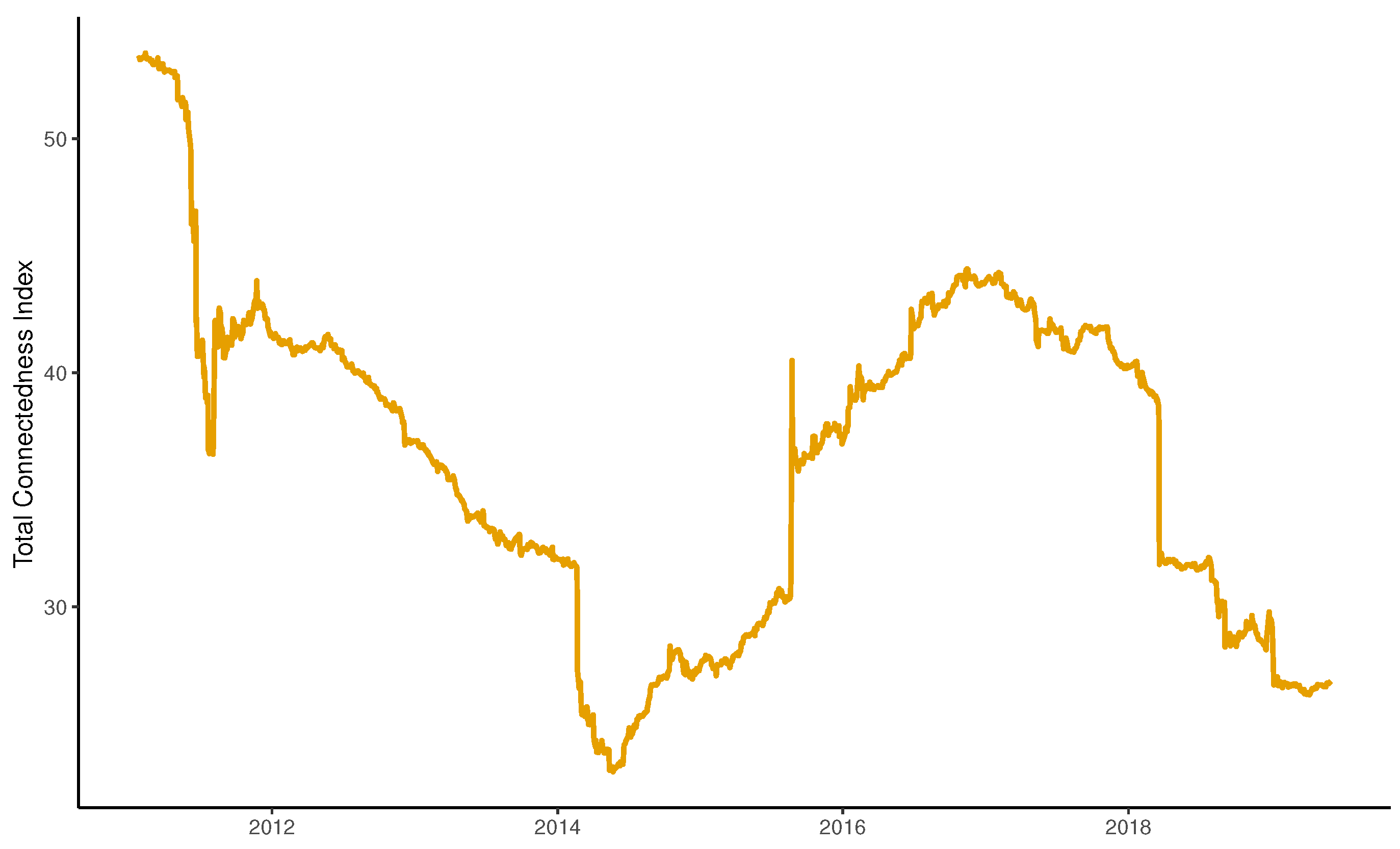
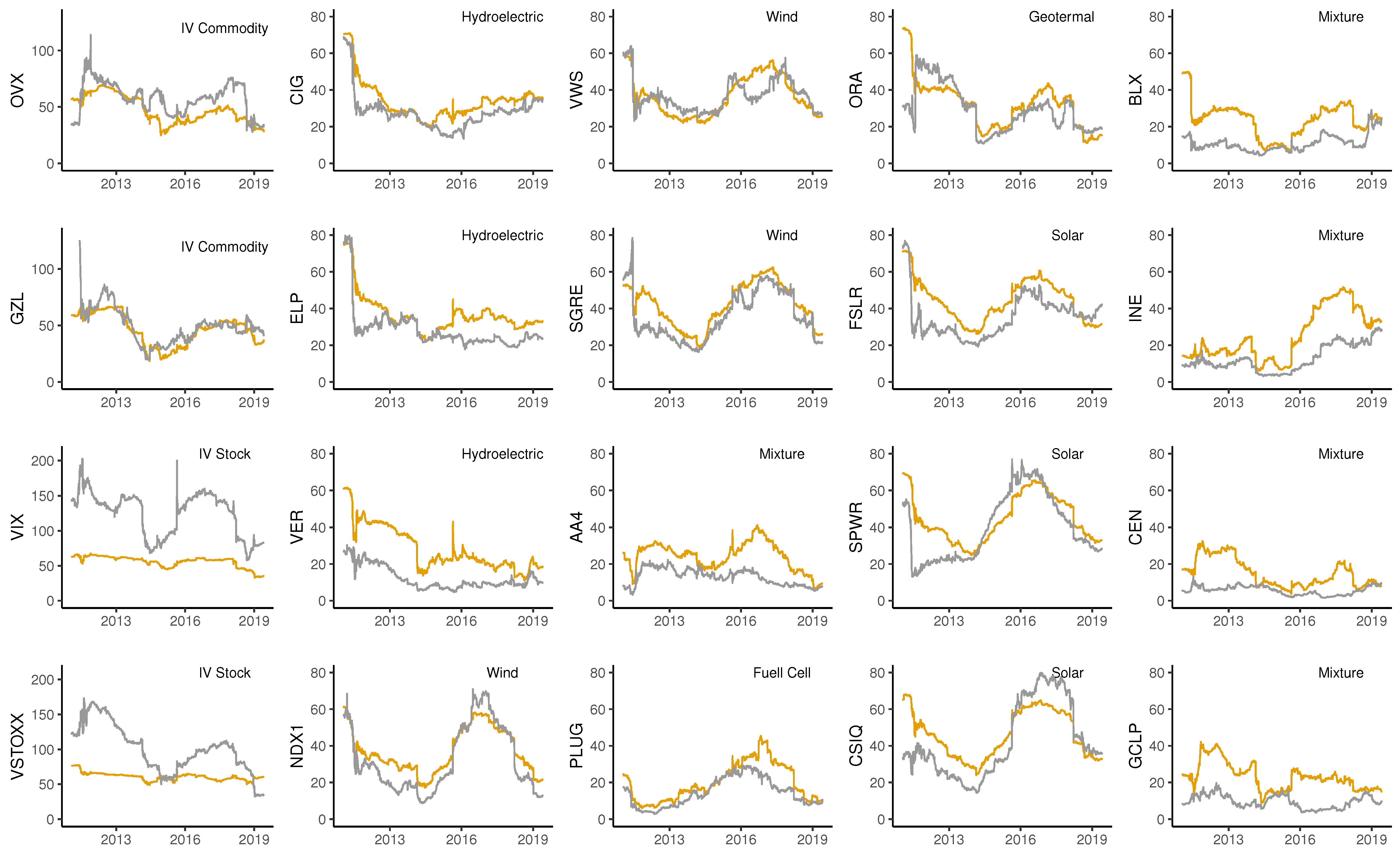
5.2. Rolling-Sample Analysis: Spillover Plots

In this section, we show the advantages of studying the dynamic behavior between volatility indices. We also present evidence that the dynamic total connectedness index C t H can distinguish peaks and falls in financial markets. Figure 2 shows a plot of the dynamic total connectedness index for the full sample. These results were obtained from a VAR model of order 1 with a rolling window of 500 days (two years). We examined the variance decomposition with a 10-step-ahead horizon. In order to determine the prediction horizon and the span of the rolling window, we followed the robustness analysis proposed by Antonakakis and Kizys [47].
Throughout the period under analysis, many changes can be observed. These changes indicate the evolution of total directional connectedness, which fluctuated widely between 25% and 65%. In the 2008 subprime crisis, we can observe the highest rate of interdependence, showing that volatility shocks are transmitted quickly through markets in times of financial stress [37]. The first period of the sample also captured the effect of the European debt crisis at the end of 2009. Subsequently, the total directional connectedness of the systems began to decrease. In the middle of 2014, political confrontations between the United States and Russia led to an increase in market tensions, spurring another rise in the index. Saudi Arabia helped the United States to pressure the Russian government by changing its policy of keeping oil prices high. As a result, the price of oil began to fall from US$100/barrel in July 2014 to US$44 in March 2015. “Black Monday”, on 24 August 2015 can be observed in Figure 2. This episode of financial turmoil led to the highest increase in oil volatility since the Subprime Crisis and tensions across global financial markets [13,16,36,41].
Figure 3 shows the estimation results, for the clean energy stocks in different subsectors, of the total directional connectedness measures “to” and “from” with gray and orange lines, respectively. In both cases, it is possible to observe that the patterns of transmission varied over time and differed between subsectors. Cross-sectional patterns are clear and particularly evident in the dynamic of “from” volatility spillovers. This result is to be expected, as clean energy stocks are receptors of shocks produced by the implied volatility indices and not the other way around. Among the main subsectors displaying the same patterns of total directional connectedness were CIG, ELP, and VER in hydroelectric energy; NDX1, VWS, and SGRE in wind energy; and FSLR, SPWR, and CSIQ in solar energy.
In summary, the total directional connectedness measures between companies in the same energy production subsector showed similar behavior; however, this behavior was very heterogeneous between different energy production subsectors over time. Thus, total directional connectedness measures in clean energy stocks are affected by inherent patterns in each subsector of production. From this finding, we conclude that it is inadvisable to characterize the behavior of clean energy stocks by simply using a global index.

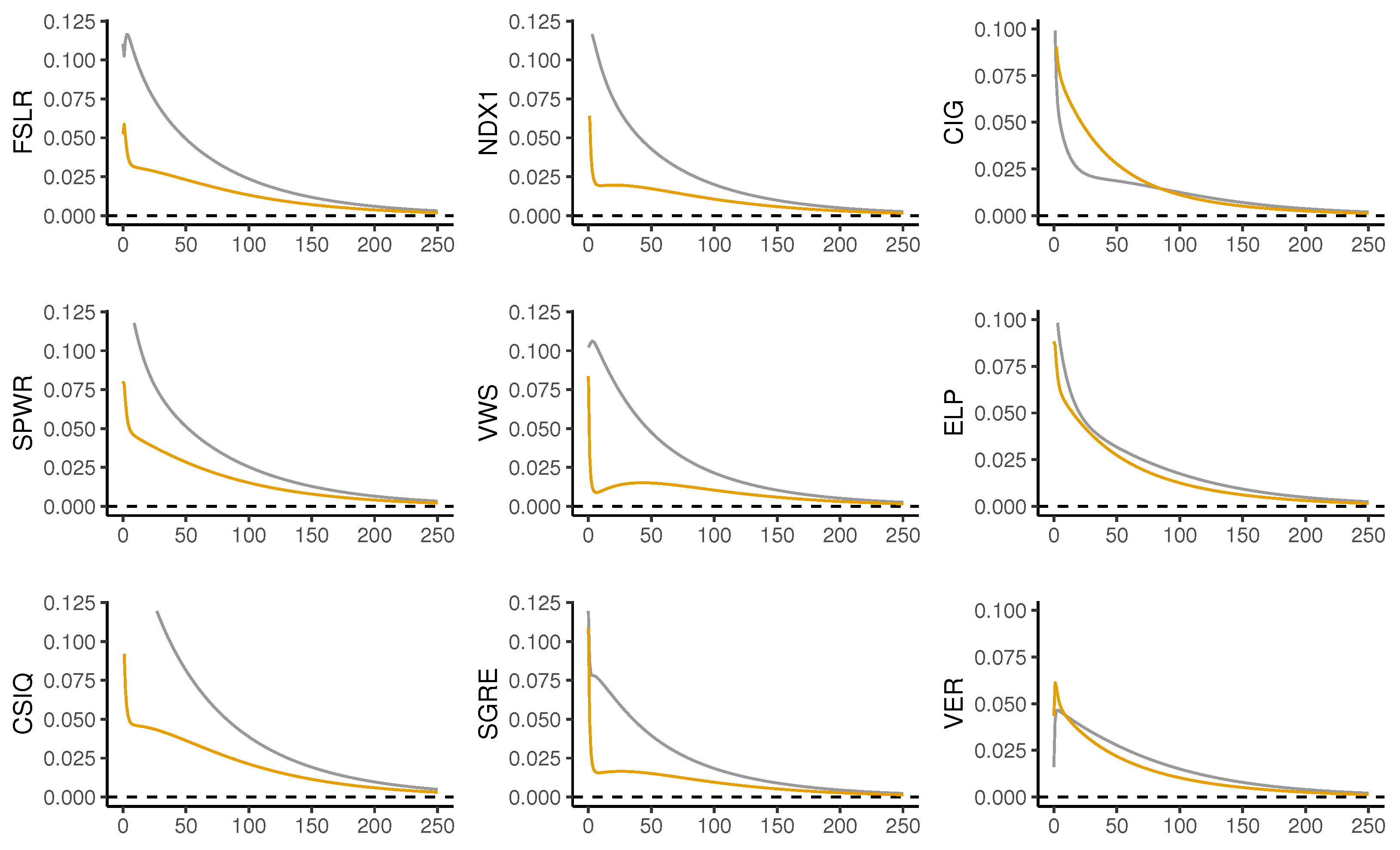
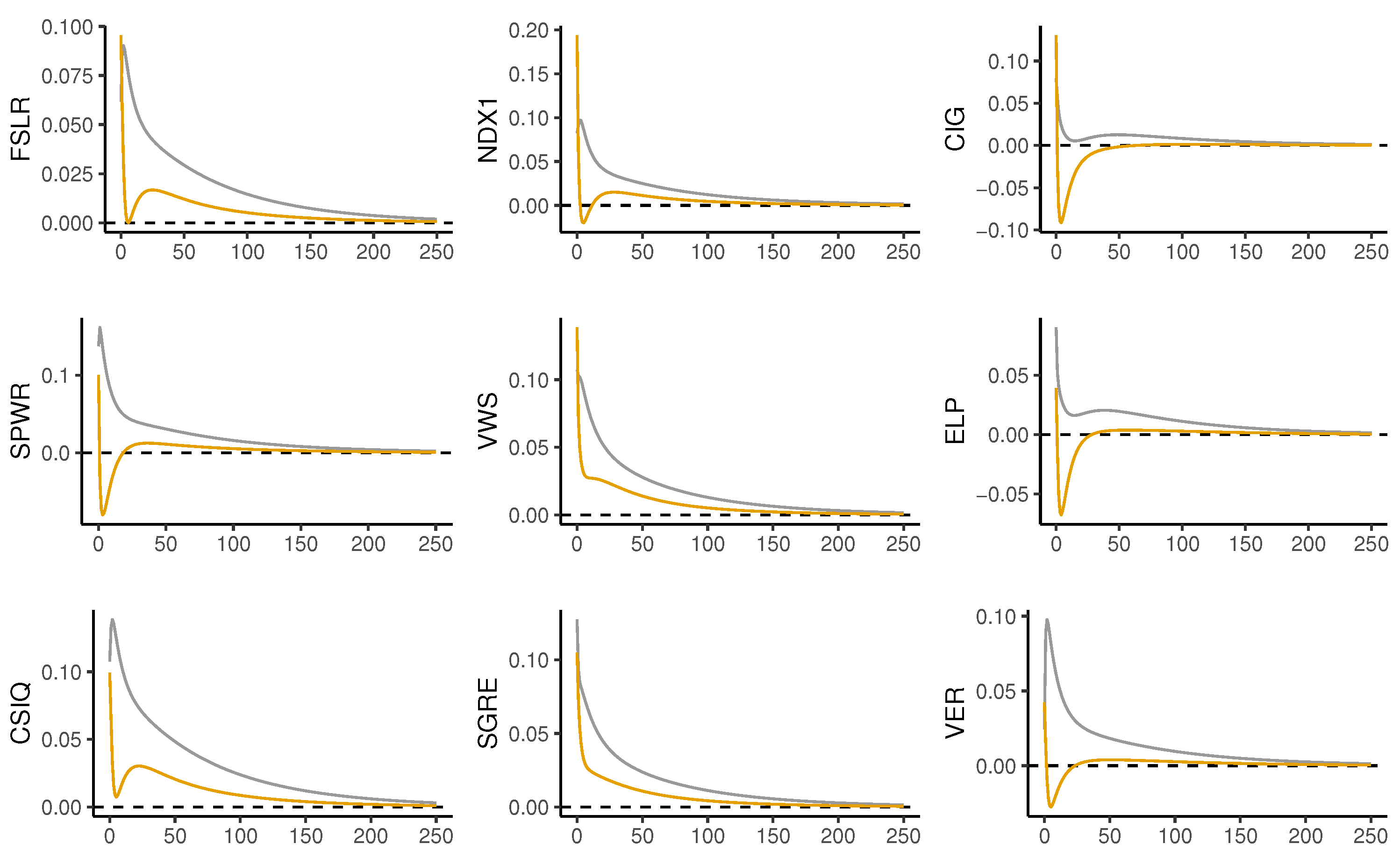
5.3. Impulse–Response Analysis

We used the estimations from our VAR model to run an impulse–response analysis between the realized volatilities of the clean energy stocks and the implied volatility indices. In the previous section, we found evidence of cross-sectional connectedness in clean energy stocks from the same subsector of production. Accordingly, we focused our impulse–response analysis on identifying whether there was similar response behaviors, in the clusters previously identified, when faced with an impulse in the implied volatilities of commodities and when faced with an impulse in the implied volatilities of the global stock market indices. The results are significant at the 95% level and shown in Figure 4 and Figure 5, respectively. Graphics including the confidence interval are available from the author upon request.
On one hand, the left and center columns of Figure 4 exhibit the impulse–response functions for solar and wind energy companies, respectively. We can observe that shocks coming from the implied volatility of gold generated higher and more persistent impacts than shocks coming from the implied volatility of oil; for instance, the impulse–response functions seemed to stabilize after five months for G V Z . For many companies, their response to a shock in O V X had a more abrupt rate of decline, decaying after one month. On the other hand, in the right column of Figure 4, we show the impulse–response functions for hydroelectric companies. In this case, the estimations show a similar response to shocks coming from both commodities, G V Z and O V X , typically stabilizing after four months. This finding implies that, for this subsector of production, both the future market expectations of the price of gold and oil can be considered as relevant factors. In Table 4, it is possible to observe that, among the clean energy stocks, connectedness with O V X was only higher in the hydroelectric energy companies.
The impulse–response functions relating to the implied volatilities of the global indices and the clean energy stocks are shown in Figure 5. We observe that shocks originating in V I X had a significant impact on clean energy stocks in all subsectors of production. For solar and wind energy companies, the response Was more persistent over time; in particular, the impulse–response functions for V I X seemed to stabilize after four months, while the hydroelectric companies recuperated faster. Shocks coming from V S T O X X generated a negative response in hydroelectric energy companies and a sharper decay rate in solar and wind energy companies, stabilizing at around two months.

6. Conclusions

Clean energy is a dynamic and promising industry which has experienced rapid growth over the last decade. We used the Diebold–Yilmaz connectedness methodology to examine the connectedness between the daily realized volatility indices of 16 clean energy stocks belonging to the SPGCE and implied volatility indices of two global stock markets—the S&P 500 and the STOXX50—and two commodities—the crude oil and gold markets. In this way, we provided a detailed characterization of the connectedness of clean energy markets by investigating the heterogeneity among different subsectors of clean energy production.
The empirical findings showed that there was a unidirectional connectedness from the implied volatility indices to the realized volatility indices of clean energy stocks. Among the implied volatility indices, the future expectations of V I X and G V Z played a leading role in volatility spillovers to the clean energy stocks.
In the dynamic analysis, the time-varying total connectedness index was shown to be able to capture rises and falls in financial price volatilities, as evidenced by the interdependence of volatilities during times of financial crisis. Answering our research questions, the results revealed the heterogeneous behavior between different energy production subsectors over time. Thus, to gain complete knowledge of the interdependence between clean energy stocks, it is necessary to separately examine the volatility dynamics of clean energy stocks from different subsectors of production. Furthermore, relating how clean energy stock prices of different production subsectors are influenced by changes in prices of the main financial and commodity markets, we obtained the following results: Through an impulse–response analysis, we confirmed the impact of shocks in V I X on the realized volatility of clean energy stocks. In terms of commodities, volatility shocks in G V Z produced higher and more persistent responses in the realized volatility of clean energy stocks.
As a policy implication of our research findings, portfolio managers can gain a better understanding of the complex behavior of each clean energy stock by incorporating stylized facts related to each production subsector, in order to effectively promote clean energy investment promoting economic development in this sector. Thus, the construction of optimal diversification strategies should consider the management of investment portfolios at a disaggregated level, taking into account each productive subsector’s distinctive characteristics. Our research findings are consistent with Reboredo [22] and Pham [10], who are the first empirical studies to document the heterogeneity of the different clean energy production subsectors.

Author Contributions

All authors contributed equally to all aspects of the research reported in this paper. All authors have read and agreed to the published version of the manuscript.

Funding

The authors acknowledge the Chilean CONICYT funding agency for its financial support (FONDECYT 1180672) for this project.

Conflicts of Interest

The authors declare no conflict of interest.

References

  1. Mejdoub, H.; Ghorbel, A. Conditional dependence between oil price and stock prices of renewable energy: A vine copula approach. Econ. Political Stud. 2018, 6, 176–193. [Google Scholar] [CrossRef]
  2. Amran, Y.A.; Amran, Y.M.; Alyousef, R.; Alabduljabbar, H. Renewable and sustainable energy production in Saudi Arabia according to Saudi Vision 2030; Current status and future prospects. J. Clean. Prod. 2019, 247, 119602. [Google Scholar] [CrossRef]
  3. Valadkhani, A.; Smyth, R.; Nguyen, J. Effects of primary energy consumption on CO2 emissions under optimal thresholds: Evidence from sixty countries over the last half century. Energy Econ. 2019, 80, 680–690. [Google Scholar] [CrossRef]
  4. Bhattacharya, M.; Paramati, S.R.; Ozturk, I.; Bhattacharya, S. The effect of renewable energy consumption on economic growth: Evidence from top 38 countries. Appl. Energy 2016, 162, 733–741. [Google Scholar] [CrossRef]
  5. Zeppini, P.; Van Den Bergh, J.C. Global competition dynamics of fossil fuels and renewable energy under climate policies and peak oil: A behavioural model. Energy Policy 2020, 136, 110907. [Google Scholar] [CrossRef]
  6. Malik, K.; Rahman, S.M.; Khondaker, A.N.; Abubakar, I.R.; Aina, Y.A.; Hasan, M.A. Renewable energy utilization to promote sustainability in GCC countries: Policies, drivers, and barriers. Environ. Sci. Pollut. Res. 2019, 26, 20798–20814. [Google Scholar] [CrossRef] [PubMed]
  7. Dutta, A.; Bouri, E.; Das, D.; Roubaud, D. Assessment and optimization of clean energy equity risks and commodity price volatility indexes: Implications for sustainability. J. Clean. Prod. 2020, 243, 118669. [Google Scholar] [CrossRef]
  8. Kocaarslan, B.; Soytas, U. Asymmetric pass-through between oil prices and the stock prices of clean energy firms: New evidence from a nonlinear analysis. Energy Rep. 2019, 5, 117–125. [Google Scholar] [CrossRef]
  9. Webb, J. New lamps for old: Financialised governance of cities and clean energy. J. Cult. Econ. 2019, 12, 286–298. [Google Scholar] [CrossRef]
  10. Pham, L. Do all clean energy stocks respond homogeneously to oil price? Energy Econ. 2019, 81, 355–379. [Google Scholar] [CrossRef]
  11. Dutta, A.; Bouri, E.; Noor, M.H. Return and volatility linkages between CO2 emission and clean energy stock prices. Energy 2018, 164, 803–810. [Google Scholar] [CrossRef]
  12. Kyritsis, E.; Serletis, A. Oil Prices and the Renewable Energy Sector. Energy J. 2019, 40, 337–364. [Google Scholar] [CrossRef]
  13. Maghyereh, A.I.; Awartani, B.; Abdoh, H. The co-movement between oil and clean energy stocks: A wavelet-based analysis of horizon associations. Energy 2019, 169, 895–913. [Google Scholar] [CrossRef]
  14. Reboredo, J.C.; Ugolini, A. The impact of energy prices on clean energy stock prices. A multivariate quantile dependence approach. Energy Econ. 2018, 76, 136–152. [Google Scholar] [CrossRef]
  15. Bouri, E.; Jalkh, N.; Dutta, A.; Salah, G. Gold and crude oil as safe-haven assets for clean energy stock indices: Blended copulas approach. Energy 2019, 178, 544–553. [Google Scholar]
  16. Ahmad, W.; Sadorsky, P.; Sharma, A. Optimal hedge ratios for clean energy equities. Econ. Model. 2018, 72, 278–295. [Google Scholar] [CrossRef]
  17. Dutta, A. Oil price uncertainty and clean energy stock returns: New evidence from crude oil volatility index. J. Clean. Prod. 2017, 164, 1157–1166. [Google Scholar] [CrossRef]
  18. Park, J.; Ratti, R.A. Oil price shocks and stock markets in the US and 13 European countries. Energy Econ. 2008, 30, 2587–2608. [Google Scholar] [CrossRef]
  19. Kilian, L.; Park, C. The impact of oil price shocks on the US stock market. Int. Econ. Rev. 2009, 50, 1267–1287. [Google Scholar] [CrossRef]
  20. Ahmad, W. An analysis of directional spillover between crude oil prices and stock prices of clean energy and technology companies. Res. Int. Bus. Financ. 2017, 42, 376–389. [Google Scholar] [CrossRef]
  21. Henriques, I.; Sadorsky, P. Oil prices and the stock prices of alternative energy companies. Energy Econ. 2008, 30, 998–1010. [Google Scholar] [CrossRef]
  22. Reboredo, J.C. Is there dependence and systemic risk between oil and renewable energy stock prices? Energy Econ. 2015, 48, 32–45. [Google Scholar] [CrossRef]
  23. Kumar, S.; Managi, S.; Matsuda, A. Stock prices of clean energy firms, oil and carbon markets: A vector autoregressive analysis. Energy Econ. 2012, 34, 215–226. [Google Scholar] [CrossRef]
  24. Tully, E.; Lucey, B.M. A power GARCH examination of the gold market. Res. Int. Bus. Financ. 2007, 21, 316–325. [Google Scholar] [CrossRef]
  25. Shahzad, S.J.H.; Raza, N.; Shahbaz, M.; Ali, A. Dependence of stock markets with gold and bonds under bullish and bearish market states. Resour. Policy 2017, 52, 308–319. [Google Scholar] [CrossRef] [Green Version]
  26. Diebold, F.X.; Yılmaz, K. On the network topology of variance decompositions: Measuring the connectedness of financial firms. J. Econom. 2014, 182, 119–134. [Google Scholar] [CrossRef] [Green Version]
  27. Managi, S.; Okimoto, T. Does the price of oil interact with clean energy prices in the stock. Jpn. World Econ. 2013, 27, 1–9. [Google Scholar] [CrossRef] [Green Version]
  28. Sadorsky, P. Correlations and volatility spillovers between oil prices and the stock prices of clean energy and technology companies. Energy Econ. 2012, 34, 248–255. [Google Scholar] [CrossRef]
  29. Demirer, M.; Diebold, F.X.; Liu, L.; Yilmaz, K. Estimating global bank network connectedness. J. Appl. Econom. 2018, 33, 1–15. [Google Scholar] [CrossRef]
  30. Ahmad, W. On the dynamic dependence and investment performance of crude oil and clean energy stocks. Res. Int. Bus. Financ. 2017, 42, 376–389. [Google Scholar] [CrossRef]
  31. Ahmad, W.; Rais, S. Time-varying spillover and the portfolio diversification implications of clean energy equity with commodities and financial assets. Emerg. Mark. Financ. Trade 2018, 54, 1837–1855. [Google Scholar] [CrossRef]
  32. Sadorsky, P. Modeling renewable energy company risk. Energy Policy 2012, 40, 39–48. [Google Scholar] [CrossRef]
  33. Bondia, R.; Ghosh, S.; Kanjilal, K. International crude oil prices and the stock prices of clean energy and technology companies: Evidence from non-linear cointegration tests with unknown structural breaks. Energy 2016, 101, 558–565. [Google Scholar] [CrossRef]
  34. Reboredo, J.C.; Rivera-Castro, M.A.; Ugolini, A. Wavelet-based test of co-movement and causality between oil and renewable energy stock prices. Energy Econ. 2017, 61, 241–252. [Google Scholar] [CrossRef]
  35. Yahşi, M.; Çanakoğlu, E.; Ağralı, S. Carbon price forecasting models based on big data analytics. Carbon Manag. 2019, 10, 175–187. [Google Scholar] [CrossRef]
  36. Maghyereh, A.I.; Awartani, B.; Bouri, E. The directional volatility connectedness between crude oil and equity markets: New evidence from implied volatility indexes. Energy Econ. 2016, 57, 78–93. [Google Scholar] [CrossRef] [Green Version]
  37. Awartani, B.; Aktham, M.; Cherif, G. The connectedness between crude oil and financial markets: Evidence from implied volatility indices. J. Commod. Mark. 2016, 4, 56–69. [Google Scholar] [CrossRef] [Green Version]
  38. Garman, M.B.; Klass, M.J. On the estimation of security price volatilities from historical data. J. Bus. 1980, 53, 67–78. [Google Scholar] [CrossRef]
  39. Pesaran, H.H.; Shin, Y. Generalized impulse response analysis in linear multivariate models. Econ. Lett. 1998, 58, 17–29. [Google Scholar] [CrossRef]
  40. Diebold, F.X.; Yilmaz, K. Measuring financial asset return and volatility spillovers, with application to global equity markets. Econ. J. 2009, 119, 158–171. [Google Scholar] [CrossRef] [Green Version]
  41. Diebold, F.X.; Liu, L.; Yilmaz, K. Commodity Connectedness; Technical Report; National Bureau of Economic Research: Cambridge, MA, USA, 2017.
  42. Polat, O. Systemic risk contagion in FX market: A frequency connectedness and network analysis. Bull. Econ. Res. 2019, 71, 585–598. [Google Scholar] [CrossRef]
  43. Gupta, D.; Kamilla, U. Dynamic linkages between implied volatility indices of developed and emerging financial markets: An econometric approach. Glob. Bus. Rev. 2015, 16, 46S–57S. [Google Scholar] [CrossRef]
  44. Ding, L.; Huang, Y.; Pu, X. Volatility linkage across global equity markets. Glob. Financ. J. 2014, 25, 71–89. [Google Scholar] [CrossRef]
  45. Shu, H.C.; Chang, J.H. Spillovers of volatility index: Evidence from US, European, and Asian stock markets. Appl. Econ. 2019, 51, 2070–2083. [Google Scholar] [CrossRef]
  46. Sarwar, G. Interrelations in market fears of US and European equity markets. N. Am. J. Econ. Financ. 2020, 41, 101136. [Google Scholar] [CrossRef]
  47. Antonakakis, N.; Kizys, R. Dynamic spillovers between commodity and currency markets. Int. Rev. Financ. Anal. 2015, 41, 303–319. [Google Scholar] [CrossRef] [Green Version]
Figure 1. Daily implied volatility time-series (IV of commodities and stocks) and the daily realized volatility time-series for 16 clean energy stocks belonging to the SPGCE (highlighting the sector of production) of each company over the full sample period extending from June 2008 to June 2019. The labels utilized for the description of the companies are detailed in Table 2.
Energies 13 03705 g001
Figure 2. The total connectedness index ( C t H ), indicating total connectedness among the stock volatilities for the time period from June 2008 to June 2019. A two-year rolling estimation window is utilized and a 10-step-ahead predictive horizon is used for the underlying variance decomposition.
Energies 13 03705 g002
Figure 3. Total directional connectedness C j H transmitted (“to”, gray line) from the market j to the rest of the system and total directional connectedness C i H received (“from”, orange line) by market i from the rest of the system for the period June 2008 to June 2019. A two-year rolling estimation window is utilized and a 10-step-ahead predictive horizon is used for the underlying variance decomposition.
Energies 13 03705 g003
Figure 4. Impulse–response analysis of clean energy stocks, clustered by sector of production, when faced with a shock in GVZ (gray line) and in OVX (orange line) one year ahead (250 days). Left, center, and right columns correspond to solar, wind, and hydroelectric energy companies, respectively.
Energies 13 03705 g004
Figure 5. Impulse–response analysis of clean energy stocks, clustered by sector of production, when faced with a shock in VIX (gray line) and in VSTOXX (orange line) one year ahead (250 days). The left, center, and right columns correspond to solar, wind, and hydroelectric energy companies, respectively.
Energies 13 03705 g005
Table 1. Methodologies and indices used for empirical analyses in different articles.
Econometric MethodologyReferenceSpecificationIndices
VARKumar et al. [23]VARECO, SPGCE, NEX, PSE, Oil, Carbon, Interest Rate, S&P 500
Managi and Okimoto [27]Markov Switching VARECO, PSE, Oil, Interest Rate
VolatilitySadorsky [28]BEKK, Diagonal, DCC, CCCECO, PSE, Oil
Ahmad et al. [16]DCC, ADCC, GO-GARCHECO, Oil, Gold, VIX, OVX, Carbon, Bond
Dutta et al. [11]VAR-GARCH, DCC-GARCHECO, ERIX, Carbon
Maghyereh et al. [13]waveled MGARCH-DCCECO, Oil, FTSE ET50
Kyritsis and Serletis [12]VAR-GARCH in meanECO, SPGCE, NEX, PSE, Oil
Dutta et al. [7]DCC-GARCHECO, SPGCE, MAC, OVX, GVZ, VXSLV
CopulasReboredo [22]TGARCH- CopulaECO, SPGCE, ERIX, WIND, SOLAR, TECH, Oil
Mejdoub and Ghorbel [1]TGARCH-Vine CopulaECO, SPGCE, NEX, Oil
Reboredo and Ugolini [14]Multivariate Vine CopulaECO, ERIX, Oil, Natural Gas, Coal, Electricity, S&P 500, Euro Stoxx 50
Bouri et al. [15]EVT-CopulasECO, SPGCE, Oil, Gold
MixedSadorsky [32]Beta model (CAPME extension)PBW, Oil
Bondia et al. [33]Threshold Cointegration Test, Granger Causality.NEX, PSE, Oil, Interest Rate
Reboredo et al. [34]Wavelet based-test, Granger CausalityECO, SPGCE, ERIX, Oil, WIND, SOLAR, TECH
Dutta [17]Range-based volatility measures.ECO, Oil, OVX, Carbon
Yahşi et al. [35]Random Forest, RegressionSPGCE, DAX, Oil, Natural Gas, Coal, Carbon, Electricity
Diebold-Yilmaz ConnectednessAhmad [30]Diebold-Yilmaz connectedness, BEKK, DCC, CCCECO, PSE, Oil
Ahmad and Rais [31]Diebold-Yilmaz connectedness, ADCCNEX, PSE, Oil, Heating, Gasoline, DJIMI, Market Indexes: WORLD-DS, US-DS, EUROPE-DS.
Pham [10]Diebold-Yilmaz connectedness, DCC, ADCC, GO-GARCHOil, NASDAQ OMX Clean Energy Indices.
Notes: ECO: Wilder Hill Clean Energy Index. NEX: Wilder Hill New Energy Global Innovation Index. SPGCE: S&P Global Clean Energy Index. PBW: Wilder Hill Clean Energy ETF. PSE: NYSE Arca Technology Index. EUA: European Union Allowances. ERIX: European renewable energy index. NE: China’s new energy index. WIND: NYSE Bloomberg Global Wind Energy Index, SOLAR: NYSE Bloomberg Global Solar Energy, TECH: NYSE Bloomberg Global Energy Smart Technologies Index, MAC: MAC global solar energy stock.
Table 2. Description of the 16 individual clean energy stock prices belonging to the SPGCE index.
NameTickerFoundedSubsector
Cia Energetica de Minas Gerais Prf ADRCIGBrazil, 1952Hydro (Electric power)
Companhia Paranaense de EnergiaELPBrazil, 1954Hydro (Electric power)
VERBUND AGVERAustria, 1947Hydro (Electric power)
Nordex SENDX1Germany, 1985Wind
Vestas Wind Systems ASVWSDenmark, 1945Wind
Siemens Gamesa Renewable EnergySGRESpain, 1976Wind
FalckrenewablesAA4Italy, 2002Mixture
PlugpowerPLUGUSA, 1997Fuell Cell
Ormat TechnologiesORAUSA, 1965Geotermal
First Solar IncFSLRUSA, 1999Solar
SunpowerSPWRUSA, 1985Solar
Canadian Solar IncCSIQCanada, 2001Solar
Boralex Inc. ’A’BLXCanada, 1982Mixture
Innergex Renewable Energy IncINECanada, 1990Mixture
Contact Energy LtdCENNew Zealand, 1996Mixture
GCL Poly Energy Holdings LtdGCLPChina, 2006Mixture
Note: the table shows the name of the company, the country and year in which it was founded, and the sector of production or activity it is involved in. Companies that produce different types of energy have been labelled as ‘mixture’.
Table 3. Descriptive statistics of daily implied volatility indices and realized volatility indices.
TickerMeanStandard
Deviation
MinMaxSkewnessKurtosisJarque–
Bera
Box–
Pierce
Phillips–
Perron
OVX36.22113.76214.50098.9301.3402.3750.000.000.02
GVZ19.1457.8018.88064.5302.0625.9170.000.000.01
VIX19.3789.6249.15080.8602.5438.3620.000.000.01
VSTOXX29.95113.24511.990117.3101.7934.7060.000.000.01
CIG2.0941.2870.1608.9475.91393.8940.000.000.01
ELP1.8811.1280.36214.5753.66124.0270.000.000.01
VER1.6300.9780.15612.7432.87717.2350.000.000.01
NDX12.3621.5630.00012.3222.0836.5800.000.000.01
VWS2.1271.4770.30315.8022.85413.4270.000.000.01
SGRE2.2851.3030.42715.4252.1269.3810.000.000.01
AA42.1891.2830.29411.9971.9435.9770.000.000.01
PLUG4.3012.9210.37526.3652.3858.7420.000.000.01
ORA1.5851.1100.30419.4994.53642.9950.000.000.01
FSLR2.5991.5370.56619.2703.01816.7150.000.000.01
SPWR3.1991.7820.65718.3152.73312.5210.000.000.01
CSIQ3.5812.1390.56723.4102.76414.8360.000.000.01
BLX1.3991.1860.00016.8064.84742.2370.000.000.01
INE1.2171.1820.00016.5795.53346.3760.000.000.01
CEN0.8630.5050.0005.4731.8237.4340.000.000.01
GCLP2.8151.6330.00018.0252.51412.3950.000.000.01
Note: the last two columns show the p-values of the Jarque–Bera and Box–Pierce tests with 10 lags.
Table 4. Full-Sample Connectedness.
OVXGVZVIXVSTOXXCIGELPVERNDX1VWSSGREAA4PLUGORAFSLRSPWRCSIQBLXINECENGCLP C i H C i H
OVX61.097.0815.757.812.381.290.700.400.410.340.200.160.830.100.390.280.440.330.010.0039.001.4
GVZ4.8452.3913.5414.411.841.750.111.731.661.360.410.500.921.371.241.640.250.020.010.0147.6050.0
VIX8.7512.1345.5820.490.790.940.941.931.581.860.340.221.790.590.910.430.510.050.120.0554.4085.0
VSTOXX6.1913.2128.0940.660.790.470.371.951.992.350.890.200.740.710.470.410.290.120.100.0159.4038.0
CIG3.464.263.412.7752.3219.971.271.531.010.270.270.191.791.702.311.771.500.070.030.0947.60-2.8
ELP2.837.194.831.7218.6647.571.442.300.970.640.040.483.431.652.482.590.850.150.030.1752.40-7.2
VER2.583.059.983.293.212.9959.082.551.021.540.560.452.681.012.010.712.390.130.360.4241.00-25.6
NDX10.785.295.304.671.491.851.6460.133.323.940.941.032.931.521.952.240.200.090.160.5239.80-6.8
VWS0.344.465.896.031.120.570.783.4158.2511.070.170.422.621.970.871.130.090.330.160.3141.80-3.8
SGRE0.803.986.166.440.390.521.004.1811.3659.170.290.211.651.521.060.940.050.070.050.1840.80-7.6
AA41.080.672.414.810.500.160.371.580.590.5484.450.120.230.800.960.060.050.220.150.2615.60-10.0
PLUG0.443.831.751.270.250.470.031.420.930.330.0883.701.070.341.442.220.130.100.080.1216.20-5.2
ORA1.867.5310.676.003.174.041.302.873.392.030.160.7847.552.292.052.441.340.370.130.0452.40-20.8
FSLR0.584.684.663.581.631.440.631.143.842.390.280.532.2650.9312.716.920.350.730.110.6149.00-10.6
SPWR0.855.196.952.181.702.190.601.331.621.770.421.041.7212.5651.167.430.330.640.090.2148.80-7.6
CSIQ1.047.206.674.851.662.650.552.312.311.620.092.013.077.718.1247.000.290.330.110.4153.00-18.6
BLX1.935.705.473.164.392.482.640.950.300.310.041.532.470.351.311.1765.120.530.100.0834.80-25.4
INE1.300.232.421.110.350.080.070.090.530.070.140.780.400.040.100.490.1391.430.190.068.60-4.2
CEN0.370.601.270.470.190.220.630.810.570.260.050.100.520.390.220.550.230.0592.340.167.60-5.6
GCLP0.471.294.122.260.281.120.270.440.520.540.320.250.441.810.651.010.070.130.0983.9216.00-12.2
C j H 40.4097.60139.497.4044.8045.2015.4033.0038.0033.205.6011.0031.6038.4041.2034.409.404.402.003.80 V S I H = 38.31%
Note: C H corresponds to the total Volatility Spillover Index connectedness. Model based on a VAR of order 1. Each component ( i , j ) of the table is the estimated contribution from stock volatility j to the 10-step-ahead forecast error variance of stock volatility i. C j H is the contribution from stock market j to others. C i H is the contribution from other markets to stock volatility i.

