Super-Resolution DoA Estimation on a Co-Prime Array via Positive Atomic Norm Minimization

Abstract

A super-resolution direction-of-arrival (DoA) estimation algorithm that employs a co-prime array and positive atomic norm minimization (ANM) is proposed. To exploit larger array cardinality, the co-prime array vector is constructed by arranging elements of a correlation matrix. The positive ANM is a technique that can enhance resolution when the coefficients of the atoms are the positive real numbers. A novel optimization problem is proposed to ensure the coefficients of the atoms are the positive real numbers, and the positive ANM is employed after solving the optimization problem. The simulation results show that the proposed algorithm achieves high resolution and has lower complexity than the other ANM-based super-resolution DoA estimation algorithm.

1. Introduction

A direction-of-arrival (DoA) estimation is one of the representative research topics in the field of array signal processing and has been adopted in a various applications, such as localization and radar [1]. DoA estimation algorithms exploit the signals collected from an array of antennas and estimate the directions of the signal sources by signal processing techniques [2]. There are many factors that can evaluate the performance of the DoA estimation algorithm, and one of the key factors is resolution. The super-resolution in DoA estimation refers to a successful estimation of multiple DoAs that are closely separated [3]. For intuitive understanding, a DoA estimation performance according to the resolution is presented in Figure 1.

Traditional DoA estimation algorithms such as [4,5] have high resolution. However, they require high signal-to-noise ratios (SNRs) and large numbers of snapshots. To overcome these disadvantages, compressive sensing (CS)-based DoA estimation algorithms have been proposed [3,6,7]. Regardless of types of CS, such as basis pursuit (BP) [8] and sparse Bayesian learning (SBL) [9], CS-based DoA estimation algorithms are robust against low SNR and fewer snapshots [7]. The CS-based DoA estimation algorithms commonly form a discretized grid, which is composed of all candidates of DoA estimates. The DoAs are estimated by finding the grid components that have the highest correlations with the received signal. In practice, however, a real DoA does not match perfectly with the component of the grid. This problem is widely known as grid-mismatch, and the estimation error induced by the grid-mismatch is proportional to the step size of the grid [10].

On the other hand, the atomic norm minimization (ANM)-based DoA estimation works directly on continuous DoA and completely resolves the grid-mismatch. The ANM-based DoA estimation was first proposed in [11], and the theoretical basis of the atomic norm was established in [12]. After the proposal of the ANM, the robustness of the ANM-based algorithm against noise [13] and the gain-phase error [14] has been discussed. The ANM-based algorithm also extended to various applications, including multiple-input-multiple-output (MIMO) radar [15] and MIMO channel estimation [16,17]. The study in [18], however, has proven that the DoAs of the signals must be separated more than at least the minimum separation distance when using ANM. The minimum separation distance can be translated as the resolution limit of ANM, where the minimum separation distance is inversely proportional to the array cardinality (i.e., the effective number of antenna elements in an array).

To increase the resolution of the ANM-based DoA estimation, the following approaches can be taken into consideration. One approach to increase the resolution is to employ the sparse array metrics such as the co-prime array [19] and the nested array [20], wherein the sparse array metrics are introduced to estimate the DoAs of more signal sources than the number of antennas. The sparse array creates a virtual array whose cardinality is much larger than that of the physical array. Since the resolution is proportional to the array cardinality [18], the usage of the sparse array results in resolution improvement. The sparse array has been exploited in the seminal works of CS-based DOA estimation [21,22,23] and ANM-based DOA estimation [24,25]. The other approaches to increase the resolution were introduced in [26,27,28]. In [26], reweighted atomic norm minimization (RAM) has been proposed; RAM can achieve the resolution beyond the limit noted in [18]. However, RAM suffers from high complexity due to the iterative execution of ANM. The algorithm proposed in [27,28], which is referred to as the positive ANM, shows that the resolution can be further enhanced when the coefficients of atoms are the positive real numbers. However, the coefficients of atoms are arbitrary complex numbers in the DoA estimation scenario, wherein the atoms are array manifold vectors, and their coefficients have unknown phases. Thus, to our knowledge, there has been no case in which the positive ANM was employed for DoA estimation.

In this paper, we propose a super-resolution DoA estimation algorithm using the co-prime array and the positive ANM. Increased cardinality is exploited by using the co-prime array. To ensure that the coefficients of the atoms are positive real numbers, a novel optimization problem is derived, wherein the optimization problem also removes the noise on the co-prime array. After solving the optimization problem, the positive ANM is employed by solving semidefinite programming (SDP) derived in [27].

2. Signal Model

We assume that P uncorrelated narrowband signals impinge on the antenna array with M elements. The carrier frequency of the signal is f, and their DoAs are $\mathsf{\Theta }={\left[{\theta }_1,\dots ,{\theta }_P\right]}^T$. An array manifold vector whose DoA is $\theta$, $\mathbf{a}\left(\theta \right)$ can be given as

$$\mathbf{a}\left(\theta \right)={\left[e^{j2\pi (d_1/\lambda )cos\theta },\dots ,e^{j2\pi (d_M/\lambda )cos\theta }\right]}^T\in {\mathbb{C}}^{M\times 1},$$

(1)

where $d_m$ denotes a distance between the m-th antenna and the reference antenna, and $\lambda =c/f$. Note that c is the speed of light. ${\mathbb{C}}^{M\times 1}$ denotes a complex vector with the size of $M\times 1$, and note that this notation can also represent the complex matrix. The first antenna is the reference antenna if not noted, and hence $d_1=0$. An array manifold matrix for P signal sources, $\mathbf{A}\left(\mathsf{\Theta }\right)$ is

$$\mathbf{A}\left(\mathsf{\Theta }\right)=\left[\mathbf{a}\left({\theta }_1\right),\dots ,\mathbf{a}\left({\theta }_P\right)\right]\in {\mathbb{C}}^{M\times P}.$$

(2)

The received signal $\mathbf{X}$ can be written as

$$\mathbf{X}=\mathbf{A}\left(\mathsf{\Theta }\right)\mathbf{S}+\mathbf{N}\in {\mathbb{C}}^{M\times D},$$

(3)

where D is the number of snapshots. $\mathbf{S}={\left[{\mathbf{s}}_1,\dots ,{\mathbf{s}}_P\right]}^T$ where ${\mathbf{s}}_p\in {\mathbb{C}}^{D\times 1}$ denotes the p-th signal vector. $\mathbf{N}$ is an additive white Gaussian noise matrix whose columns follow $\mathcal{CN}({\mathbf{0}}_M,{\sigma }^2{\mathbf{I}}_M)$, where ${\mathbf{0}}_M$ is a $M\times 1$ zero vector, ${\mathbf{I}}_M$ is a $M\times M$ identity matrix, and ${\sigma }^2$ denotes the power of the noise. ${\mathbf{R}}_{\mathbf{X}}$, the correlation matrix of $\mathbf{X}$, can be defined as

$$\begin{array}{c}\hfill {\mathbf{R}}_{\mathbf{X}}=\mathbb{E}\left[\mathbf{X}{\mathbf{X}}^H\right]=\mathbf{A}\left(\mathsf{\Theta }\right){\mathbf{R}}_{\mathbf{S}}\mathbf{A}{\left(\mathsf{\Theta }\right)}^H+{\sigma }^2{\mathbf{I}}_M,\end{array}$$

(4)

where ${\mathbf{R}}_{\mathbf{S}}=\mathbb{E}\left[\mathbf{S}{\mathbf{S}}^H\right]$. Since all signal sources are uncorrelated with each other, ${\mathbf{R}}_{\mathbf{S}}$ is a diagonal matrix where its p-th diagonal element equals to the power of the p-th signal source.

We define $\mathbf{z}=\mathrm{diag}\left({\mathbf{R}}_{\mathbf{S}}\right)\in {\mathbb{R}}_{+}^{P\times 1}$, where $\mathrm{diag}(·)$ denotes a vector whose entries are diagonal elements of a given matrix, and ${\mathbb{R}}_{+}^{P\times 1}$ denotes a vector composed of positive real numbers with the size of $P\times 1$. The $(i,j)$-th element of ${\mathbf{R}}_{\mathbf{X}}$, ${\mathbf{R}}_{\mathbf{X}}(i,j)$ is given as

$$\begin{array}{cc}\hfill & {\mathbf{R}}_{\mathbf{X}}(i,j)=\hfill \\ \hfill & \left\{\begin{array}{cc}{\displaystyle {\displaystyle \sum _{p=1}^P}\mathbf{z}\left(p\right)e^{j2\pi \{(d_i-d_j)/\lambda \}cos{\theta }_p}}\hfill & \mathrm{for}i\ne j,\hfill \\ {\displaystyle {\displaystyle \sum _{p=1}^P}\mathbf{z}\left(p\right)e^{j2\pi \{(d_i-d_j)/\lambda \}cos{\theta }_p}+{\sigma }^2}\hfill & \mathrm{for}i=j,\hfill \end{array}\right.\hfill \end{array}$$

(5)

where $\mathbf{z}\left(p\right)$ is the p-th element of $\mathbf{z}$, which denotes the power of the p-th signal source and satisfies that $\mathbf{z}\left(p\right)=\mathbb{E}\left[{\mathbf{s}}_p^H{\mathbf{s}}_p\right]$.

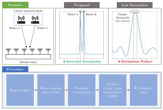
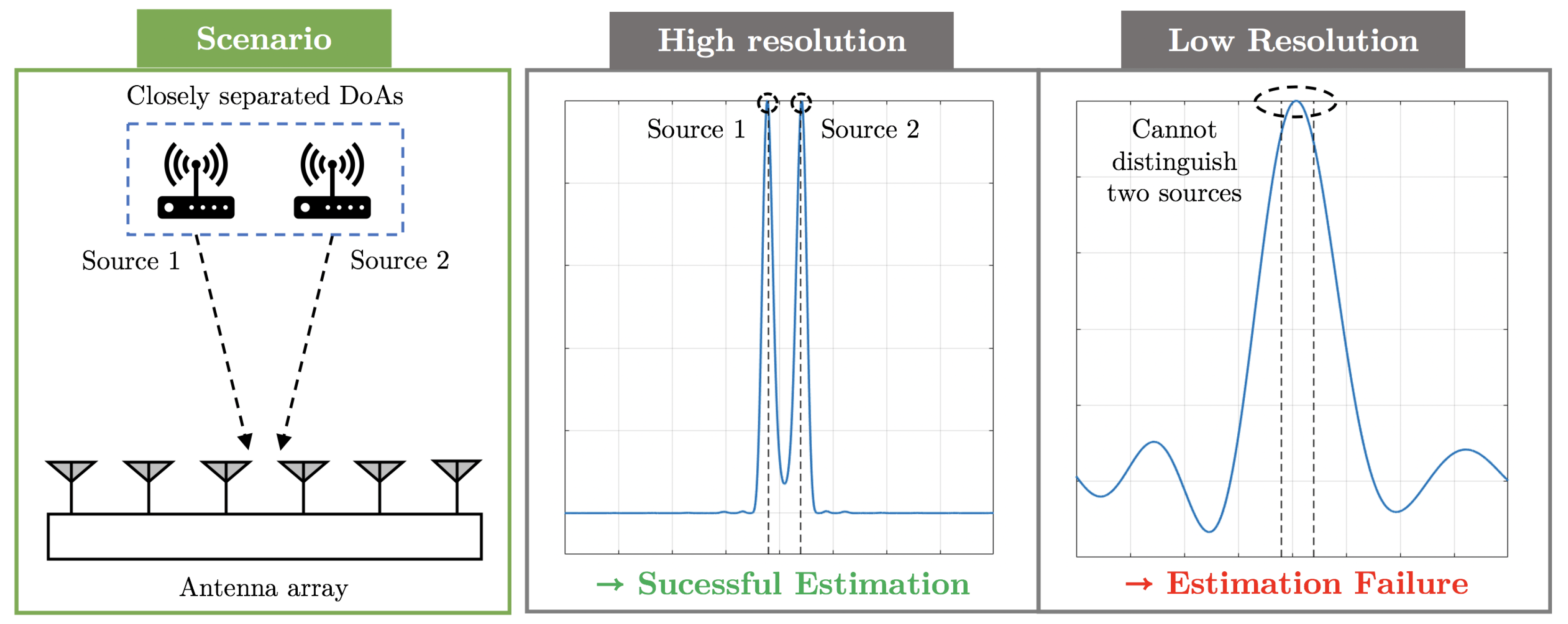
3. Super-resolution DoA Estimation on Co-Prime Array via Positive Atomic Norm Minimization

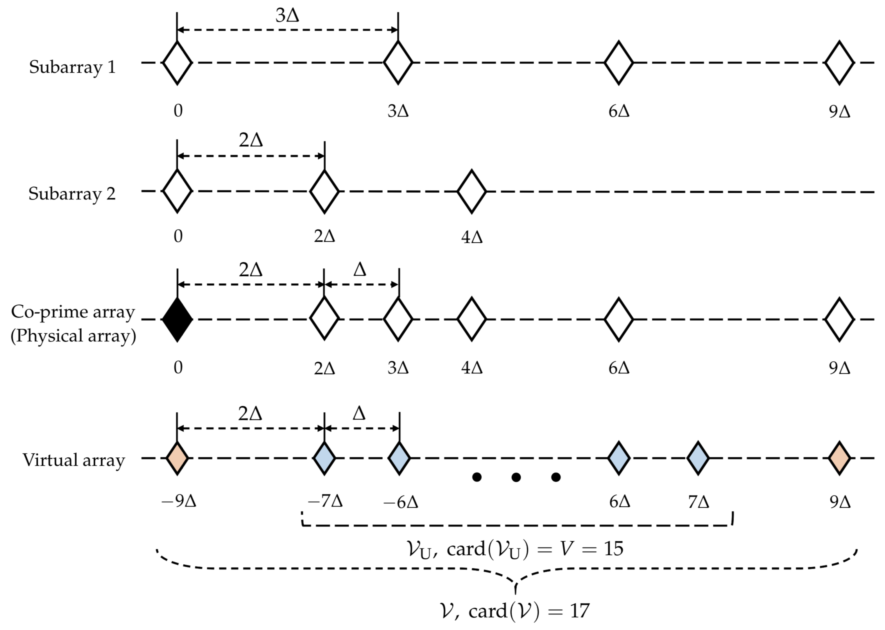
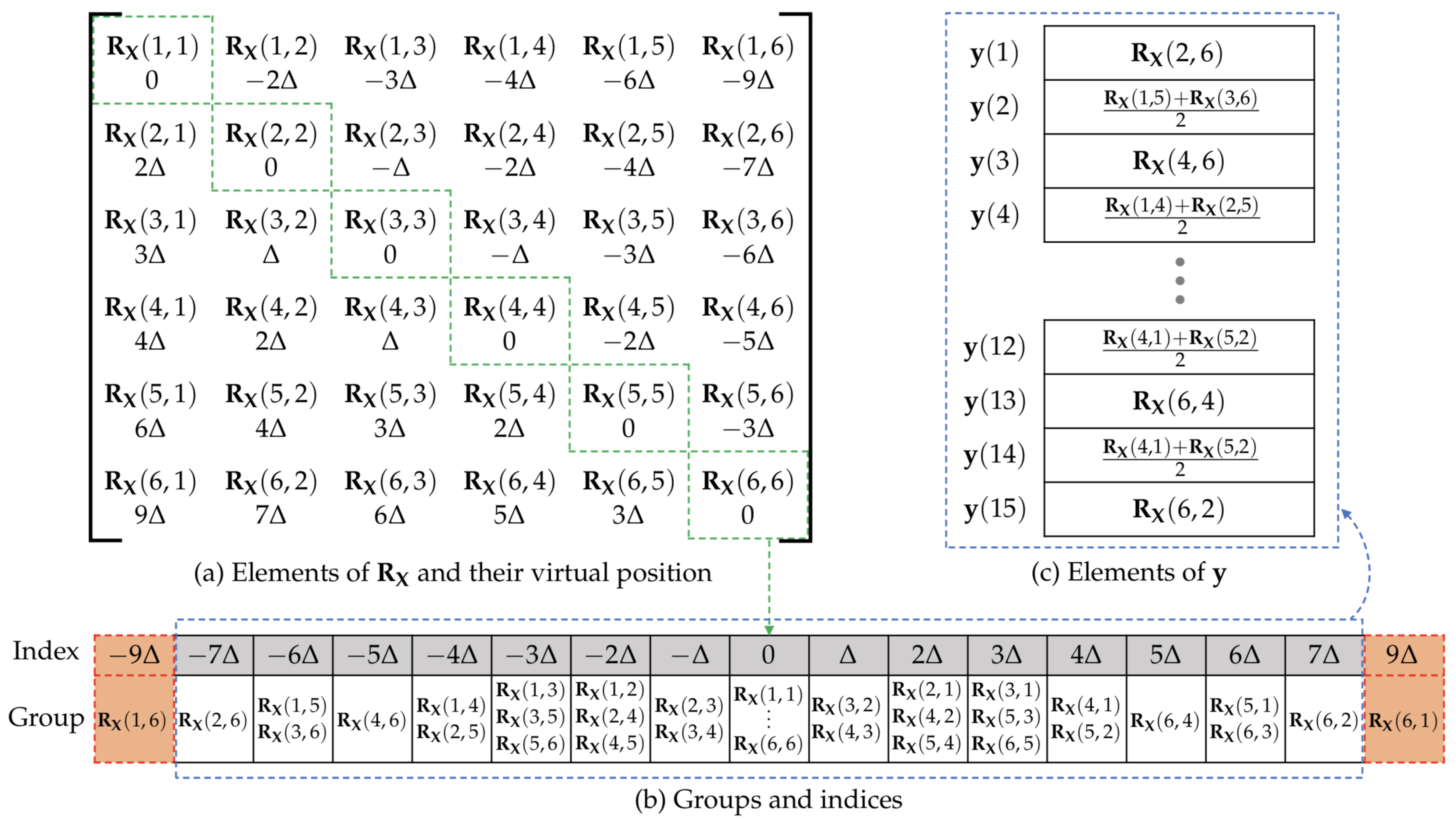
3.1. Construction of Co-Prime Array Vector

To increase the number of detectable signal sources by using the co-prime array, the placement of the antennas should follow the rule in [19], and the co-prime array vector needs to be constructed by rearranging the elements of the correlation matrix. The co-prime array is a combination of two sparse subarrays, where one subarray consists of $2M_1$ antennas spaced $M_2\Delta$ apart and the other consists of $M_2$ antennas spaced $M_1\Delta$ apart. $\Delta$ is set to a half-wavelength such that $\Delta =\lambda /2$. The structures of co-prime array and its virtual array $\mathcal{V}$ are given in Figure 2, where $M=2M_1+M_2-1$. The virtual array is the notion that is used in the seminal works of co-prime array [24,29], where it does not exist physically, yet we can obtain the effect of using larger array cardinality. The set $\mathcal{V}$ that indicates the placement of antennas in the virtual array can be defined as [19]:

$$\mathcal{V}=\left\{d_i-d_j|i,j=1,2,\dots ,M\right\}.$$

(6)

Note that some elements repeat and additional repeating elements are removed. Figure 2 shows two subarrays, the co-prime array, and the virtual array when $M_1=2$ and $M_2=3$. $\mathcal{V}$ can be split into two subsets, as in Figure 2: the placements of antenna elements which constitute a large ULA at the center, ${\mathcal{V}}_{\mathrm{U}}$, and the remaining placements. V denotes the cardinality of ${\mathcal{V}}_{\mathrm{U}}$.

The co-prime array vector $\mathbf{y}\in {\mathbb{C}}^{V\times 1}$ is constructed to obtain the cardinality of ${\mathcal{V}}_{\mathrm{U}}$ using ${\mathbf{R}}_{\mathbf{X}}$. The construction of $\mathbf{y}$ from ${\mathbf{R}}_{\mathbf{X}}$ is depicted in Figure 3. For clearer understanding, we define the term virtual position of ${\mathbf{R}}_{\mathbf{X}}(i,j)$ as $d_i-d_j$. Given the elements of ${\mathbf{R}}_{\mathbf{X}}$ and their virtual position in Figure 3a, the procedure of constructing $\mathbf{y}$ can be broken down into three steps:

• Group the elements of ${\mathbf{R}}_{\mathbf{X}}$ with the same virtual position as in Figure 3b. Note that the index in Figure 3b denotes the common virtual position of the elements within the group.
• Leave only the groups whose indices are equivalent to the elements of ${\mathcal{V}}_{\mathrm{U}}$ as in Figure 3b.
• Average the elements in remaining groups, and vectorize the averaged elements to obtain $\mathbf{y}$ as in Figure 3c.

$\mathbf{y}\in {\mathbb{C}}^{V\times 1}$ can also be rewritten as

$$\mathbf{y}={\mathbf{A}}_v\left(\mathsf{\Theta }\right)\mathbf{z}+\mathbf{e}=\widehat{\mathbf{y}}+\mathbf{e}.$$

(7)

${\mathbf{A}}_v\left(\mathsf{\Theta }\right)=\left[{\mathbf{a}}_v\left({\theta }_1\right),\dots ,{\mathbf{a}}_v\left({\theta }_P\right)\right]\in {\mathbb{C}}^{V\times P}$. ${\mathbf{a}}_v\left(\theta \right)$ is the array manifold vector whose antenna placement follows ${\mathcal{V}}_{\mathrm{U}}$, such that

$${\mathbf{a}}_v\left(\theta \right)={\left[e^{j\pi \frac{(-V+1)}{2}cos\theta },e^{j\pi \frac{(-V+3)}{2}cos\theta },\dots ,e^{j\pi \frac{(V-1)}{2}cos\theta }\right]}^T\in {\mathbb{C}}^{V\times 1},$$

(8)

Note that V is an odd number since ${\mathcal{V}}_{\mathrm{U}}$ is symmetric with respect to the reference antenna at the center. $\mathbf{e}={[0,\dots ,0,{\sigma }^2/M,0,\dots ,0]}^T\in {\mathbb{C}}^{V\times 1}$, where the element located in the middle of $\mathbf{e}$ is ${\sigma }^2/M$ and the other elements are 0. $\widehat{\mathbf{y}}={\mathbf{A}}_v\left(\mathsf{\Theta }\right)\mathbf{z}$ and $\mathbf{e}$ can be seen as the additive noise to $\widehat{\mathbf{y}}$, where $\mathbf{e}$ affects the element located in the middle of $\widehat{\mathbf{y}}$.

3.2. Super-Resolution DoA Estimation via Positive ANM

The atomic norm of $\widehat{\mathbf{y}}$, ${\parallel \widehat{\mathbf{y}}\parallel }_{\mathcal{A}}$ can be given as:

$$\begin{array}{ll}{\parallel \widehat{\mathbf{y}}\parallel }_{\mathcal{A}}& =\inf \left\{g>0:g\mathrm{conv}\left(\mathcal{A}\right)\right\}\\ & =\inf \left\{\left.{\displaystyle \sum _{l=1}^L}\left|h_l\right|\right|\widehat{\mathbf{y}}={\displaystyle \sum _{l=1}^L}{h}_l\mathit{\psi }\left({\theta }_l\right)\right\},\end{array}$$

(9)

where $\mathrm{conv}(·)$ denotes a convex of hull of a set, $\mathcal{A}$ is a set of atoms, L is the number of atoms that constitutes $\widehat{\mathbf{y}}$, and $\mathit{\psi }\left({\theta }_l\right)$ is the l-th atom. $\mathit{\psi }\left(\theta \right)={\left[1,e^{j\pi cos\theta },\dots ,e^{j\pi (V-1)cos\theta }\right]}^T\in {\mathbb{C}}^{V\times 1}$, and $\mathcal{A}=\left\{\left.\mathit{\psi }\left(\theta \right)\right|0^{°}<\theta <{180}^{°}\right\}$. $h_l$ is a coefficient of the l-th atom which satisfies $\widehat{\mathbf{y}}={\sum }_{l=1}^L{h}_l\mathit{\psi }\left({\theta }_l\right)$ for arbitrary $\left\{{\theta }_l\right\}$, where $\left\{{\theta }_l\right\}$ denotes ${\theta }_l$ for $l=1,\dots ,L$. The details of convex hull and its relationship with the atomic norm are well-explained in the seminal works of the atomic norm [11,12,27]. As shown in [27], ${\parallel \widehat{\mathbf{y}}\parallel }_{\mathcal{A}}$ can also be obtained via SDP as

$$\begin{array}{ll}{\parallel \widehat{\mathbf{y}}\parallel }_{\mathcal{A}}=& \underset{\mathbf{u},t}{min}\left\{\frac{1}{2V}\mathrm{Trace}\left(\mathrm{Toep}\left(\mathbf{u}\right)\right)+\frac{1}{2}t\right\}\\ & \mathrm{s}.\mathrm{t}.\left[\begin{array}{cc}\mathrm{Toep}\left(\mathbf{u}\right)& \widehat{\mathbf{y}}\\ {\widehat{\mathbf{y}}}^H& t\end{array}\right]⪰0,t\ge 0,\end{array}$$

(10)

where $\mathrm{Trace}(·)$ denotes the trace of a matrix, $\mathbf{u}$ is an arbitrary complex vector whose size is $V\times 1$, and $(·)⪰0$ means that a matrix is positive semidefinite. $\mathrm{Toep}\left(\mathbf{u}\right)$ is a Hermitian–Toeplitz matrix whose first column is $\mathbf{u}$ and can be given as

$$\mathrm{Toep}\left(\mathbf{u}\right)=\left[\begin{array}{cccc}\mathbf{u}\left(1\right)& {\mathbf{u}}^{\ast }\left(2\right)& \dots & {\mathbf{u}}^{\ast }\left(V\right)\\ \mathbf{u}\left(2\right)& \mathbf{u}\left(1\right)& \dots & {\mathbf{u}}^{\ast }(V-1)\\ ⋮& ⋮& \ddots & ⋮\\ \mathbf{u}\left(V\right)& \mathbf{u}(V-1)& \dots & \mathbf{u}\left(1\right)\end{array}\right]\in {\mathbb{C}}^{V\times V},$$

(11)

where ${\mathbf{u}}^{\ast }\left(v\right)$ denotes the conjugate of $\mathbf{u}\left(v\right)$. According to [27,28], the resolution in the DoA estimation can be enhanced if $\left\{h_l\right\}$ are positive real numbers, and this is called the positive ANM.

To employ the positive ANM for the resolution enhancement, two requirements should be satisfied. First, recovering $\widehat{\mathbf{y}}$ by subtracting $\mathbf{e}$ from $\mathbf{y}$ is necessary since $\mathbf{e}$ can result in inaccurate DoA estimation. Second, the positive ANM cannot be employed since $\left\{h_l\right\}$ are arbitrary complex numbers. Thus, an algorithm that recovers $\widehat{\mathbf{y}}$ and makes the coefficients of the atoms being positive, real numbers a requirement. Motivated by (10), the optimization problem that removes $\mathbf{e}$ from $\mathbf{y}$ and enables employing the positive ANM can be derived as

$$\begin{array}{l}{\displaystyle \underset{\mathbf{u},t,b}{min}}\left\{\frac{1}{2V}\mathrm{Trace}\left(\mathrm{Toep}\left(\mathbf{u}\right)\right)+\frac{1}{2}t\right\}\\ \mathrm{s}.\mathrm{t}.\left[\begin{array}{cc}\mathrm{Toep}\left(\mathbf{u}\right)& (\mathbf{y}-b\mathbf{i})\\ {(\mathbf{y}-b\mathbf{i})}^H& t\end{array}\right]⪰0,t\ge 0,b\ge 0.\end{array}$$

(12)

$\mathbf{i}={\left[0,\dots ,0,1,0,\dots ,0\right]}^T\in {\mathbb{C}}^{V\times 1}$, where the element located in the middle of $\mathbf{i}$ is 1, and otherwise 0. In (12), subtracting $b\mathbf{i}$ from $\mathbf{y}$ stands for the recovery of $\widehat{\mathbf{y}}$. By using Schur complement, the constraint of (12) can be rewritten as

$$t\mathrm{Toep}\left(\mathbf{u}\right)-(\mathbf{y}-b\mathbf{i}){(\mathbf{y}-b\mathbf{i})}^H⪰0,t\ge 0,b\ge 0.$$

(13)

This condition leads to the fact that $\mathrm{Toep}\left(\mathbf{u}\right)$ is also positive semidefinite, as it can be easily shown that $(\mathbf{y}-b\mathbf{i}){(\mathbf{y}-b\mathbf{i})}^H⪰0$. When $\mathrm{Toep}\left(\mathbf{u}\right)⪰0$, $\mathbf{u}$ can be denoted as follows by Vandermonde decomposition theorem of the positive semidefinite Toeplitz matrix [30].

$$\mathbf{u}={\displaystyle \sum _{r=1}^R}{c}_r\mathit{\psi }\left({\theta }_r\right),c_r>0,r=1,\dots ,R,$$

(14)

where R is the rank of $\mathrm{Toep}\left(\mathbf{u}\right)$, and $c_r$ is the coefficient of the r-th atom of $\mathbf{u}$, which is a positive real number. Since $c_r>0$, the positive ANM can be employed by using $\mathbf{u}$. Furthermore, ${\mathbf{u}}^{\star }$, the optimal solution of $\mathbf{u}$ in (12) can be given as ${\mathbf{u}}^{\star }\approx {\sum }_{p=1}^P\mathbf{z}\left(p\right)\mathit{\psi }\left({\theta }_p\right)$ when (12) is accurately solved [11]. It can be seen that the formation of ${\mathbf{u}}^{\star }$ is equivalent to that of $\widehat{\mathbf{y}}$, except that the coefficients of the atoms are the positive real numbers. Given that the formation of ${\mathbf{u}}^{\star }$, the DoAs can be accurately estimated by employing the positive ANM with ${\mathbf{u}}^{\star }$. As shown in [27], the positive ANM using ${\mathbf{u}}^{\star }$ can be represented as SDP as follows.

$$\begin{array}{l}\underset{\mathbf{q},\mathbf{H}}{max}\Re \left({\mathbf{q}}^H{\mathbf{u}}^{\star }\right)\\ \mathrm{s}.\mathrm{t}.\mathbf{H}⪰0,\\ {\displaystyle \sum _{i=1}^{V-s}}\mathbf{H}(i,i+s)+\frac{\mathbf{q}(s+1)}{2}=\left\{\begin{array}{cc}1,\hfill & s=0,\hfill \\ 0,\hfill & s=1,\dots ,V-1,\hfill \end{array}\right.\end{array}$$

(15)

where $\Re (·)$ denotes a real part of given number. By letting ${\mathbf{q}}^{\star }$ denote the optimal solution of $\mathbf{q}$ in (15), the DoAs can be estimated by finding largest peaks from spatial spectrum $f\left(\theta \right)$ which is

$$f\left(\theta \right)={\mathbf{q}}^{\star }\mathit{\psi }{\left(\theta \right)}^H,\mathrm{for}{0}^{°}<\theta <{180}^{°}.$$

(16)

By letting ${\widehat{\theta }}_p$ denote the p-th estimated DoA, the pseudocode of the proposed algorithm can be given as Algorithm 1.

Algorithm 1 A super-resolution DoA estimation on a co-prime array via positive ANM.

Input: : $\mathbf{X}$ Output: : ${\widehat{\theta }}_p,p=1,\dots ,P$  ${\mathbf{R}}_{\mathbf{X}}\approx \mathbf{X}{\mathbf{X}}^H/T$;  Construct $\mathbf{y}$ according to the steps in Figure 3;  Calculate ${\mathbf{u}}^{\star }$ via (12);  Calculate ${\mathbf{q}}^{\star }$ via (15);  $f\left(\theta \right)={\mathbf{q}}^{\star }\mathit{\psi }{\left(\theta \right)}^H,\mathrm{for}{0}^{°}\le \theta <{180}^{°}$;  Find P largest peaks from $f\left(\theta \right)$ to estimate ${\widehat{\theta }}_p,p=1,\dots ,P$;

4. Simulation Results and Discussion

4.1. Simulation Settings

In this section, the performance comparison between the proposed algorithm, the classic ANM [11], and RAM [26] is presented. For the implementation of RAM, the number of iterations L is fixed to 5. Note that the algorithms based on the classic ANM and the RAM also employ the co-prime array. The co-prime array with $M_1=3$, $M_2=5$ is used. In this case, the antenna elements are physically located as $\left[0,3,5,6,9,10,12,15,20,25\right]\Delta$, where $\Delta =\lambda /2$. Under this array configuration, $V=35$. The number of snapshots $D=1000$, and ${\mathbf{R}}_{\mathbf{X}}\approx \mathbf{X}{\mathbf{X}}^H/D$. The signal-to-noise ratio (SNR) is set to 10 dB, where it is defined as follows.

$$\mathrm{SNR}=\frac{\mathrm{Trace}\left({\mathbf{R}}_{\mathbf{S}}\right)}{{\sigma }^2}=\frac{1}{{\sigma }^2}{\displaystyle \sum _{p=1}^P}\mathbf{z}\left(p\right).$$

(17)

The root mean square error (RMSE) is defined as

$$\mathrm{RMSE}=\sqrt{\frac{1}{PQ}{\sum }_{q=1}^Q\left\{{\sum }_{p=1}^P{\left({\widehat{\theta }}_p^q-{\theta }_p^q\right)}^2\right\}},$$

(18)

where Q is the number of trials for RMSE calculation, and ${\theta }_p^q$, ${\widehat{\theta }}_p^q$ respectively denote the real DoA and the estimated DoA of the p-th signal source on the q-th trial. To solve (12), (15), the classic ANM and the RAM CVX [31] are used for the optimization.

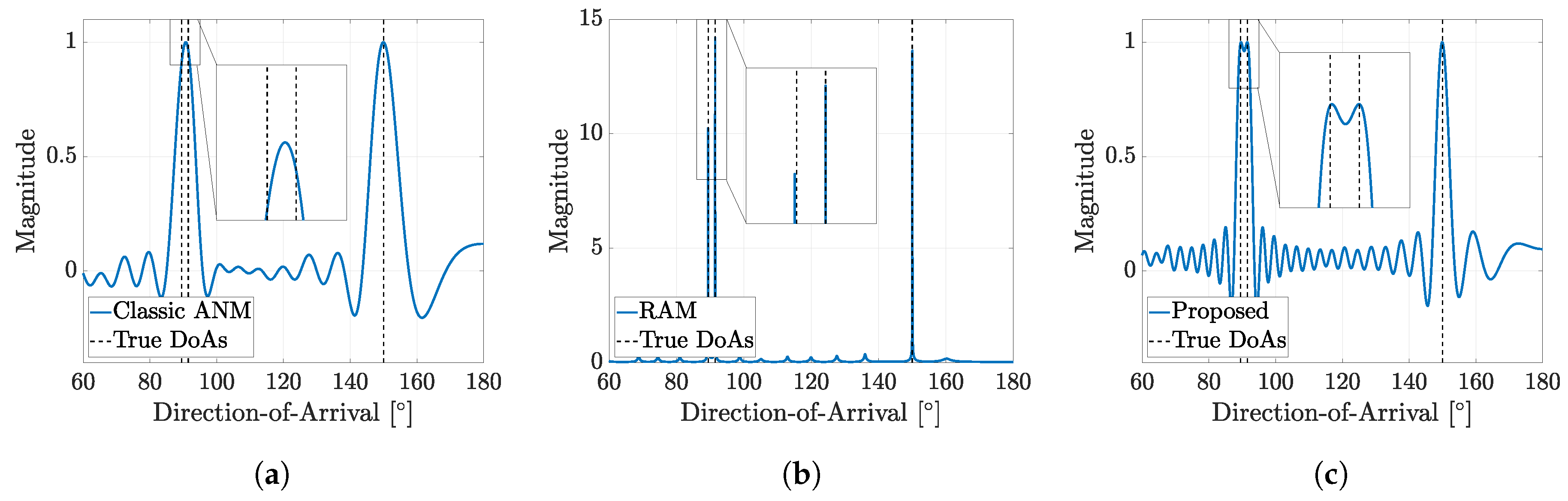
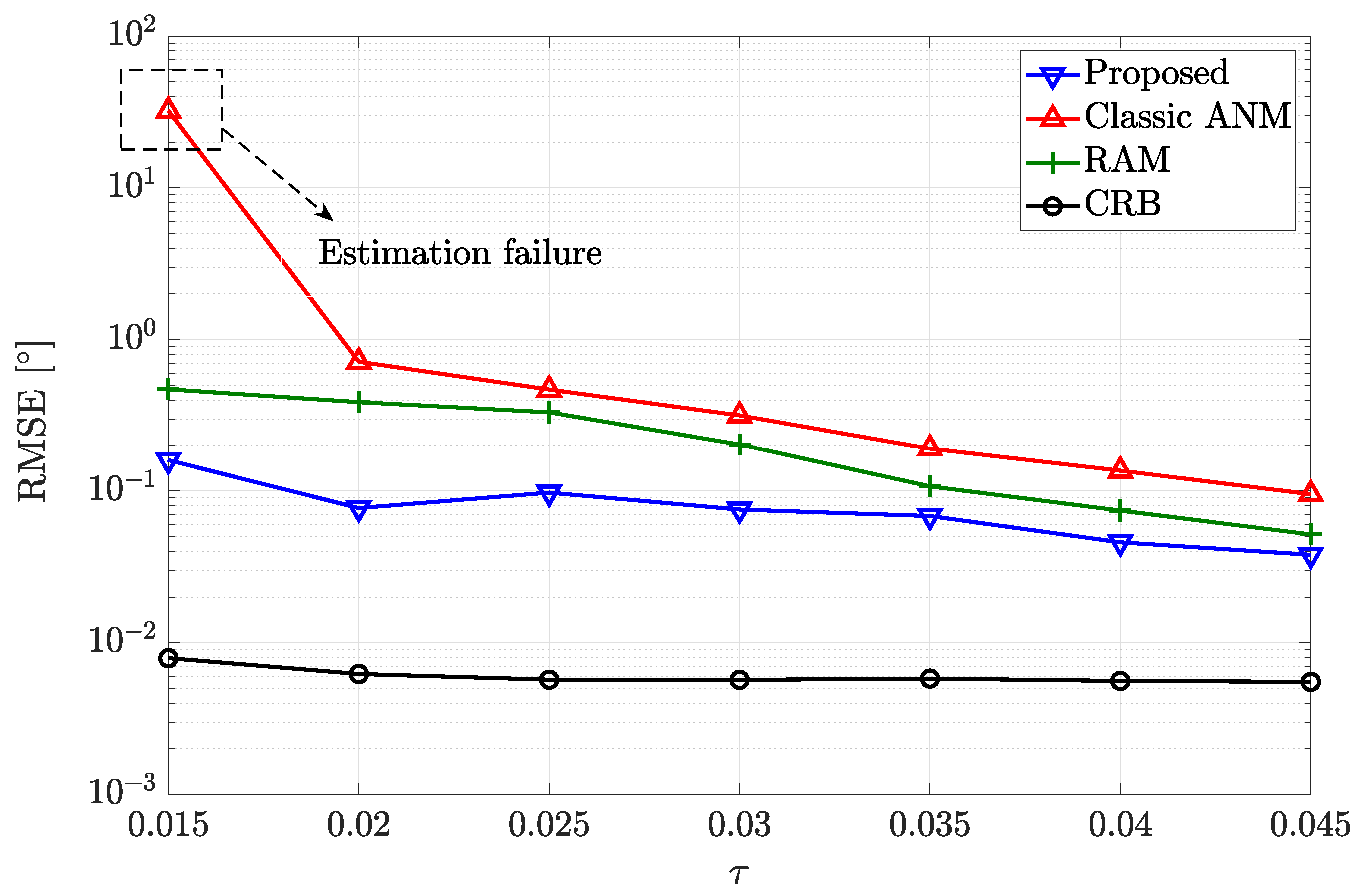
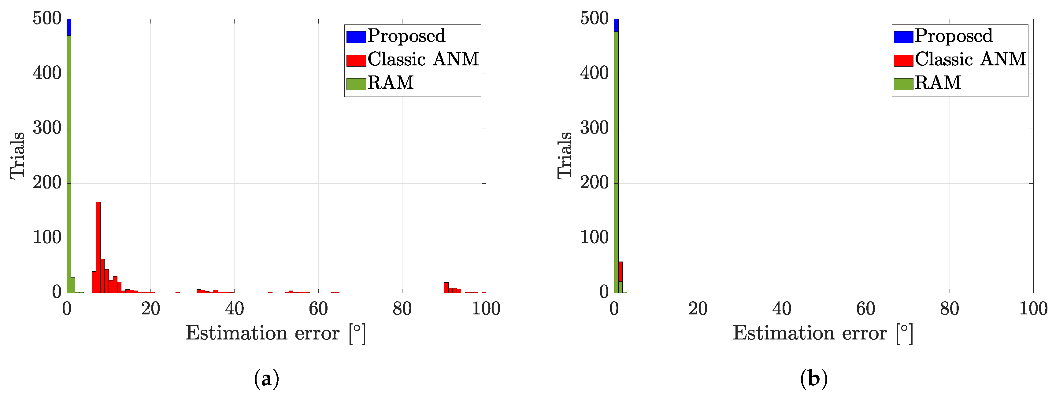
4.2. Analysis of Results and Discussion

Figure 4 presents the spectra of the classic ANM, the RAM, and the proposed algorithm. The spectrum of the proposed algorithm refers to $f\left(\theta \right)$, while the spectrum of the classic ANM is derived from the dual problem of (10), and the spectrum of the RAM refers to the weighting function in [26]. $\mathsf{\Theta }={\left[89.5°,91.5°,{150}^{°}\right]}^T$, such that DoAs of two adjacent signal sources are close while the other DoA is far from those of adjacent signal sources. Figure 4 shows that the proposed algorithm and the RAM successfully estimate two adjacent DoAs, while the classic ANM cannot. Since the DoA estimation algorithm with high resolution can estimate adjacent DoAs and the algorithms with low resolution cannot, we can tell that the proposed algorithm and RAM have higher resolutions than the classic ANM.

However, the numerical result cannot be drawn by comparing the spectra. Thus, we present the RMSE and the histogram of the estimation errors when the difference between two adjacent DoAs varies. We define a distance between two adjacent DoAs $\tau$ as $\tau =\left|(cos{\theta }_1-cos{\theta }_2)/2\right|$, where $\tau$ is used as a criterion of resolution in [11,18,27]. Note that $\tau$ is proportional to the difference between ${\theta }_1$ and ${\theta }_2$ as $\tau$ becomes 0 when ${\theta }_1={\theta }_2$. Figure 5 presents the root mean square error (RMSE) result versus $\tau$ and the Cramer–Rao bound (CRB). Here, $\mathbf{z}={\left[1,1\right]}^T$, and two DoAs are chosen randomly at each iteration. The CRB is derived by using the theorem in [32]. Figure 5 shows that the proposed algorithm has superior accuracy over the classic ANM and the RAM at every $\tau$. When $\tau =0.015$, the proposed algorithm and the RAM successfully estimate the DoAs that the classic ANM fails to estimate. Although the RMSEs of all algorithms commonly drop as $\tau$ increases, the RMSE cannot fall below CRB.

Since the RMSE does not show the estimation error of each trial, the histograms of the estimation error of each trial when $\tau =0.015$ and $\tau =0.02$ are presented in Figure 6. Note that the estimation error of the q-th trial is given as $\sqrt{{\sum }_{p=1}^P{({\widehat{\theta }}_p^q-{\theta }_p^q)}^2/P}$, and the histograms for $\tau \ge 0.025$ are omitted since the estimations of all algorithms are accurate such that the histograms do not provide meaningful statistics. In Figure 6a, the classic ANM totally fails to estimate DoAs properly, while the estimations of the proposed algorithm and RAM are accurate. In Figure 6b, the estimations of all algorithms are accurate, but the proposed algorithm shows slight superiority over the others. From Figure 5 and Figure 6, it can be considered that the proposed algorithm has good resolution since the proposed algorithm is more accurate than the other algorithms when the DoAs are closely separated.

The complexities and the average computation times of DoA estimation algorithms are given in

Table 1. The complexities and the average computation times of DoA estimation algorithms.

Algorithm	Complexity	Computation Time
Proposed	$O\left({(V+1)}^{3.5}\right)+O\left(V{(V+1)}^{3.5}\right)$	2.55 s
Classic ANM [11]	$O\left(V{(V+1)}^{3.5}\right)$	1.93 s
RAM [26]	$O\left(LV{(V+1)}^{3.5}\right)$	4.14 s

. For computation, Intel CPU i5-7500 (3.40 GHz) and 16 GB RAM were used. The number of iterations for RAM, L, was set to five. The complexities of the proposed algorithm, classic ANM, and RAM can be calculated using the analysis in [33]; the complexity of the SDP is derived in [33]. Note that the complexity of the proposed algorithm is a summation of the complexities of (12) and (15), where the complexity of (12) is $O\left({(V+1)}^{3.5}\right)$ and the complexity of (15) is $O\left(V{(V+1)}^{3.5}\right)$. Since the proposed algorithm requires solving (12) and (15), and RAM requires iterations, the complexities of the proposed algorithm and RAM are higher than that of the classic ANM. Although the proposed algorithm is more complex than the classic ANM, the proposed algorithm has advantages in resolution while having lower complexity than RAM.

5. Conclusions

In this paper, we propose the super-resolution DoA estimation algorithm using the co-prime array and the positive ANM. To increase the cardinality of an array, the co-prime array vector is constructed by arranging elements of correlation matrix. The existing SDP formulation for the ANM-based DoA estimation is modified such that the positive ANM can be applied by Vandermonde decomposition theorem, and the estimation accuracy is improved by removing the noise on the co-prime array vector. Simulation results show that the proposed algorithm has notable merits in both resolution and complexity compared to other ANM-based DoA estimation algorithms. We expect the proposed algorithm to be extended to azimuth and elevation estimation on the planar array or to the practical applications, including localization on vehicular networks and automotive radar.

References

1. Chen, J.C.; Yao, K.; Hudson, R.E. Source localization and beamforming. IEEE Signal Process. Mag. 2002, 19, 30–39. [Google Scholar] [CrossRef] [Green Version]
2. Krim, H.; Viberg, M. Two decades of array signal processing research: The parametric approach. IEEE Signal Process. Mag. 1996, 13, 67–94. [Google Scholar] [CrossRef]
3. Malioutov, D.; Cetin, M.; Willsky, A.S. A sparse signal reconstruction perspective for source localization with sensor arrays. IEEE Trans. Signal Process. 2005, 53, 3010–3022. [Google Scholar] [CrossRef] [Green Version]
4. Schmidt, R. Multiple emitter location and signal parameter estimation. IEEE Trans. Ant. Propag. 1986, 34, 276–280. [Google Scholar] [CrossRef] [Green Version]
5. Roy, R.; Kailath, T. ESPRIT-estimation of signal parameters via rotational invariance techniques. IEEE Trans. Acoust. Speech Signal Process. 1989, 37, 984–995. [Google Scholar] [CrossRef] [Green Version]
6. Liu, Z.; Huang, Z.; Zhou, Y. Direction-of-arrival estimation of wideband signals via covariance matrix sparse representation. IEEE Trans. Signal Process. 2011, 59, 4256–4270. [Google Scholar] [CrossRef]
7. Shen, Q.; Liu, W.; Cui, W.; Wu, S. Underdetermined DOA estimation under the compressive sensing framework: A review. IEEE Access 2016, 4, 8865–8878. [Google Scholar] [CrossRef]
8. Chen, S.S.; Donoho, D.L.; Saunders, M.A. Atomic decomposition by basis pursuit. SIAM J. Sci. Comput. 1999, 20, 33–61. [Google Scholar] [CrossRef]
9. Wipf, D.P.; Rao, B.D. Sparse Bayesian learning for basis selection. IEEE Trans. Signal Process. 2004, 52, 2153–2164. [Google Scholar] [CrossRef]
10. Chi, Y.; Scharf, L.L.; Pezeshki, A.; Calderbank, A.R. Sensitivity to basis mismatch in compressed sensing. IEEE Trans. Signal Process. 2011, 59, 2182–2195. [Google Scholar] [CrossRef]
11. Tang, G.; Bhaskar, B.N.; Shah, P.; Recht, B. Compressed sensing off the grid. IEEE Trans. Inf. Theory 2013, 59, 7465–7490. [Google Scholar] [CrossRef] [Green Version]
12. Chandrasekaran, V.; Recht, B.; Parrilo, P.A.; Willsky, A.S. The convex geometry of linear inverse problems. Found. Comput. Math. 2012, 12, 805–849. [Google Scholar] [CrossRef]
13. Bhaskar, B.N.; Tang, G.; Recht, B. Atomic norm denoising with applications to line spectral estimation. IEEE Trans. Signal Process. 2013, 61, 5987–5999. [Google Scholar] [CrossRef] [Green Version]
14. Chen, P.; Cao, Z.; Chen, Z. A new atomic norm for DOA estimation with gain-phase errors. arXiv 2019, arXiv:eess.SP/1910.02207. [Google Scholar]
15. Tang, W.; Jiang, H.; Pang, S. Grid-free DOD and DOA estimation for MIMO radar via duality-based 2D atomic norm minimization. IEEE Access 2019, 7, 60827–60836. [Google Scholar] [CrossRef]
16. Tsai, Y.; Zheng, L.; Wang, X. Millimeter-wave beamformed full-dimensional MIMO channel estimation based on atomic norm minimization. IEEE Trans. Commun. 2018, 66, 6150–6163. [Google Scholar] [CrossRef]
17. Chu, H.; Zheng, L.; Wang, X. Super-resolution mmwave channel estimation for generalized spatial modulation systems. IEEE J. Sel. Topics Signal Process. 2019, 13, 1336–1347. [Google Scholar] [CrossRef]
18. Candès, E.; Fernandez-Granda, C. Towards a mathematical theory of super-resolution. Commun. Pure Appl. Math. 2014, 67. [Google Scholar] [CrossRef] [Green Version]
19. Vaidyanathan, P.P.; Pal, P. Sparse sensing with co-prime samplers and arrays. IEEE Trans. Signal Process. 2011, 59, 573–586. [Google Scholar] [CrossRef]
20. Pal, P.; Vaidyanathan, P.P. Nested arrays: A novel approach to array processing with enhanced degrees of freedom. IEEE Trans. Signal Process. 2010, 58, 4167–4181. [Google Scholar] [CrossRef] [Green Version]
21. Qin, S.; Zhang, Y.D.; Amin, M.G. Generalized coprime array configurations for direction-of-arrival estimation. IEEE Trans. Signal Process. 2015, 63, 1377–1390. [Google Scholar] [CrossRef]
22. Shen, Q.; Cui, W.; Liu, W.; Wu, S.; Zhang, Y.D.; Amin, M.G. Underdetermined wideband DOA estimation of off-grid sources employing the difference co-array concept. Signal Process. 2017, 130, 299–304. [Google Scholar] [CrossRef] [Green Version]
23. Shi, Y.; Mao, X.; Zhao, C.; Liu, Y. Underdetermined DOA estimation for wideband signals via joint sparse signal reconstruction. IEEE Signal Process. Lett. 2019, 26, 1541–1545. [Google Scholar] [CrossRef]
24. Zhou, C.; Gu, Y.; Fan, X.; Shi, Z.; Mao, G.; Zhang, Y.D. Direction-of-arrival estimation for coprime array via virtual array interpolation. IEEE Trans. Signal Process. 2018, 66, 5956–5971. [Google Scholar] [CrossRef]
25. Cui, Y.; Wang, J.; Qi, J.; Zhang, Z.; Zhu, J. Underdetermined DOA estimation of wideband LFM signals based on gridless sparse reconstruction in the FRF domain. Sensors 2019, 19, 2383. [Google Scholar] [CrossRef] [Green Version]
26. Yang, Z.; Xie, L. Enhancing sparsity and resolution via reweighted atomic norm minimization. IEEE Trans. Signal Process. 2016, 64, 995–1006. [Google Scholar] [CrossRef]
27. Chi, Y.; Ferreira Da Costa, M. Harnessing sparsity over the continuum: Atomic norm minimization for superresolution. IEEE Signal Process. Mag. 2020, 37, 39–57. [Google Scholar] [CrossRef] [Green Version]
28. Chi, Y. Convex relaxations of spectral sparsity for robust super-resolution and line spectrum estimation. In Proceedings of the Wavelets and Sparsity XVII, San Diego, CA, USA, 6–9 August 2017; Volume 10394, pp. 314–321. [Google Scholar] [CrossRef]
29. He, Z.; Shi, Z.; Huang, L.; So, H.C. Underdetermined DOA estimation for wideband signals using robust sparse covariance fitting. IEEE Signal Process. Lett. 2015, 22, 435–439. [Google Scholar] [CrossRef]
30. Yang, Z.; Xie, L.; Stoica, P. Vandermonde decomposition of multilevel Toeplitz matrices with application to multidimensional super-resolution. IEEE Trans. Inf. Theory 2016, 62, 3685–3701. [Google Scholar] [CrossRef] [Green Version]
31. Grant, M.; Boyd, S. CVX: Matlab Software for Disciplined Convex Programming, Version 2.1. Available online: http://cvxr.com/cvx (accessed on 7 October 2019).
32. Stoica, P.; Larsson, E.G.; Gershman, A.B. The stochastic CRB for array processing: A textbook derivation. IEEE Signal Process. Lett. 2001, 8, 148–150. [Google Scholar] [CrossRef]
33. Pólik, I.; Terlaky, T. Interior point methods for nonlinear optimization. In Nonlinear Optimization; Di Pillo, G., Schoen, F., Eds.; Springer: Berlin/Heidelberg, Germany, 2010; pp. 215–276. [Google Scholar] [CrossRef] [Green Version]
Figure 1. A graphical representation of high resolution and low resolution direction-of-arrival (DoA) estimation.
Energies 13 03609 g001
Figure 2. An example of the co-prime array and V for M 1 = 2 and M 2 = 3 . The black antenna is a reference antenna which has an overlapped position in two subarrays. Sets of blue antennas and red antennas in V respectively denote V U and the remaining placement.
Energies 13 03609 g002
Figure 3. The construction of y using R X when M 1 = 2 and M 2 = 3 . The green, red, and blue dotted lines respectively denote the first step, the second step, and the third step of constructing y . In (a), the variable beneath every element of R X is the virtual position of the corresponding element.
Energies 13 03609 g003
Figure 4. Spectrums of DoA estimation algorithms when z = 0.3 , 0.4 , 0.5 T and Θ = 89.5 ° , 91.5 ° , 150 ° T . The boxed areas show the magnified spectrum. (a) Classic ANM [11]. (b) RAM [26]. (c) Proposed algorithm.
Energies 13 03609 g004
Figure 5. The RMSEs of the proposed algorithm, the classic ANM, and the RAM versus τ . A total of 500 trials are conducted. When τ = 0.015 , the classic ANM fails to estimate DoAs of two adjacent signal sources.
Energies 13 03609 g005
Figure 6. The histograms of the estimation error of each trial when τ = 0.015 and τ = 0.02 . A total of 500 trials were conducted to draw the histogram. (a) τ = 0.015 , (b) τ = 0.02 .
Energies 13 03609 g006