Article

Distributed Machine Learning on Dynamic Power System Data Features to Improve Resiliency for the Purpose of Self-Healing

1
The Lines Company, Te Kuiti 3910, New Zealand
2
Rocket Lab, Auckland 1060, New Zealand
3
School of Engineering, Computer and Mathematical Sciences, Auckland University of Technology, Auckland 1010, New Zealand
*
Author to whom correspondence should be addressed.
Energies 2020, 13(13), 3494; https://doi.org/10.3390/en13133494
Submission received: 7 June 2020 / Revised: 2 July 2020 / Accepted: 2 July 2020 / Published: 6 July 2020
(This article belongs to the Special Issue AI Applications to Power Systems)

Abstract

:
Numerous online methods for post-fault restoration have been tested on different types of systems. Modern power systems are usually operated at design limits and therefore more prone to post-fault instability. However, traditional online methods often struggle to accurately identify events from time series data, as pattern-recognition in a stochastic post-fault dynamic scenario requires fast and accurate fault identification in order to safely restore the system. One of the most prominent methods of pattern-recognition is machine learning. However, machine learning alone is neither sufficient nor accurate enough for making decisions with time series data. This article analyses the application of feature selection to assist a machine learning algorithm to make better decisions in order to restore a multi-machine network which has become islanded due to faults. Within an islanded multi-machine system the number of attributes significantly increases, which makes application of machine learning algorithms even more erroneous. This article contributes by proposing a distributed offline-online architecture. The proposal explores the potential of introducing relevant features from a reduced time series data set, in order to accurately identify dynamic events occurring in different islands simultaneously. The identification of events helps the decision making process more accurate.

Graphical Abstract

1. Introduction

Self-healing is a lucrative feature in the service restoration process of a power system which in turn improves system resiliency. Power system resiliency often refers to the capacity of a system to maintain stability after a high impact events with minimum interruptions [1]. Such resiliency is key to achieve the objectivity of developing a Self-healing structure [2]. In the recent studies, under the category of post-fault islanding scenarios, self-healing mechanism is getting significant attention [3]. The prominent trend in addressing self-healing is established through the local or distributed control. It is because distributed control is quite effective in faster decision making. However, applying local or distributed control is quite dependent on the dynamic characteristics of the network under analysis. On the other hand, dynamic characteristics are heavily influenced by the pre-contingent stochastic parameters, fault analysis, demand response (DR) and also the performance of the algorithms assessing power system security [2,4].
In previous studies, different methods and systems have been investigated for fault detection, isolation, and service restoration (FDIR). Some of these methods are Central Controller, Distribution Automation System (DAS), Automatic Controlled Switching (ACSs), Fault Passage Indication (FPI), Corrective Voltage Control (CVC), Emergency Demand Response Program (EDRP) and more [5]. Most of these approaches are data-intensive programs. On the top of that, in a modern grid, the integration of renewable energy makes it quite impossible to comprehend the security of a system, on an online basis for all possible scenarios. Thus self-healing function can be considered a prime candidate by the systems based on machine learning algorithms, such as Artificial Neural Network (ANN), Support Vector Machine (SVM), Random forest. If the underlying events during any critical contingency are properly identified [6], the identification can lead towards developing intelligent self-healing strategies. The process can be developed through expert systems, with a large scenario based dataset. However, machine learning systems are affected by processing time and memory. Which, in a fast restoration system is not desired, especially for those grids that require adaptive online decision making. Besides, for a large network, performing the dynamic security assessment (DSA) is an increasingly complex problem affected by numerous criteria [7,8]. Under these contexts, the traditional applications of machine learning algorithms are progressively being less effective.
The modern trend dictates that the machine learning algorithms should be trained offline basis and implemented online [9]. But multi-machine systems generate large scale data. For many online DSA programs, this approach is unattractive. Therefore, previous studies often recommend alternate solutions such as dimensionality reduction, feature selection [10,11,12]. Feature selection process is implemented to modify a data set to increase the accuracy of prediction [13,14]. However, it adds redundancy in the algorithmic steps [15]. In a large-scale power system, such redundancy will be affected by the curse of dimensionality [12]. Reference [14] mitigates this problem using an energy function based feature selection. The proposed method outperforms the method that uses raw inputs to train the machine learning algorithms, considering a smaller dataset for both the cases. This strategy proves to be highly effective, but a smaller dataset is insufficient while addressing multiple stochastic scenarios. Because in a hybrid grid, stochastic parameters make it challenging to assess dynamic security using analytical approaches. One solution to address this challenge is a Monte Carlo-based simulation method. This approach can establish the stability boundary of a grid with multiple stochastic parameters [16]. Once the stability boundary is established for a coherent group of stochastic parameters, a limited data set can be used for online DSA programs. Another approach to address the curse of dimensionality is to implement dimensionality reduction based event detection methods [10]. This method can successfully differentiate oscillatory and non-oscillatory scenarios. However, the loss of other valuable information, makes it difficult for such a simplistic approach alone to address the problem of event-detection in a hybrid system [9,17].
Due to such reasons, this work proposes a method of adding a layer of extracted features from the reduced data set. The underlying motivation is to bridge this gap between dimensionality reduction and loss of information. The power system data is collected from the available generators and transmission lines under different contingencies. The data is then reduced and features are extracted. The features are then used as attributes to train a machine learning algorithm. These features help the machine learning algorithm make accurate classification under those stochastic scenarios. The performance of the algorithm has been tested through an event-based decision making process to restore a segmented grid that significantly improves system reliability. The novelty of the process has been further justified by comparing the proposed algorithm with some existing methods. In summary, the overall contributions of this work are as follows:
  • Development of a feature selection based event detection algorithm for a multi-machine based grid, that can be sectionalized under duress. The proposed algorithm is prepared for the segmented power system used in this study. Despite not being a generic solution for all types of grids the algorithm introduces novelty in the decision making process.
  • In larger systems, the curse of dimensionality poses a bigger threat in applying machine learning algorithms, specially for making decisions. The proposed method, by implementing feature extraction on a reduced data set, addresses those challenges and enables an effective decision making scheme.

2. System Under Consideration

An IEEE-39 bus 10-machine test system as shown in Figure 1 is used in this study [18]. During a rotor angle instability the 39-bus test system can be divided into several independent islands. In this study these islands are considered as independent and locally controlled multi-machine systems when disconnected. In order to establish a relationship between the generator model and the constant impedance load model, classical energy functions were used [14];
M i d 2 δ i d t 2 + D i d δ i d t = P i j = 1 , j i m ( C i j sin δ i j + D i j cos δ i j ) ,
where P i is the active power of the i-th machine, M i is the moment of inertia of the i-th machine, D i is the damping co-efficient, m is the number of synchronous generators. δ i is the rotor angle of the i-th generator. C i j and D i j are the function of transfer conductance and susceptance of the reduced network. The per unit inertia constant of each of these generators is H = 1 2 M ω , where ω is the synchronous speed.
The proposed power system does not to have any energy storage. It considers a conventional droop characteristics for the primary frequency and voltage control. The primary control in a standalone grid that does not have any storage unit, may cause frequency deviation even if the system remains at a steady state condition. Therefore, a secondary control is also imposed that acts on the deviations observed over the primary control and tries to balance the system. The secondary control has a slower dynamics than the primary control, the idea behind that is to introduce a decoupling mechanism between these two [19].
In order to do data analysis the dynamic data is produced from the synchronous generators. The generators are controlled by a multi-band power system stabilizer (PSS) model and a governor [20,21]. The governor of each generator is modeled as a tandem-compound steam prime mover system. The overall simulation is carried out using Matlab-Simulink [22,23]. PSS are the local controllers on synchronous machines. These are quite effective in eliminating system oscillations. However, tuning the set-points for a PSS, is usually carried out via analytical calculations. In a hybrid system, where the distributed energy generation and consumption are rapidly varied, a critical three-phase fault can easily disrupt the process of damping the oscillation. It is because analytical calculations often do not capture the stochastic nature of standalone system. Therefore, a three tier hierarchical control, where the top layer deals with the probabilistic nature of a system, can bring significant improvement [19]. In this study, a supervised secondary control scheme is implemented that modifies the reference for active power generation in the turbine governor. This action helps reducing the rotor speed deviation, which is crucial for the pre-tuned set-points of the multiband-PSS, to yield result in a post-contingent scenario. The proposed supervised controller is based on machine learning algorithms. The supervised secondary controller has been implemented on each generator through a distributed architecture. This distribution is based on the machine data available in a post-contingent segment. The initial feedback data to trigger the supervised secondary control is taken from the deviation in rotor angle of the individual machine [24].
The system is designed to have rotor angle instability during a critical contingency. When such a contingency is noticed, the system can be divided into multiple operation-autonomous islands, which is necessary to eliminate the instability [25]. The method applies an unsupervised machine learning based controlled islanding mechanism that utilizes coherency based grouping from historical database. The method is further discussed in the later sections of this study.
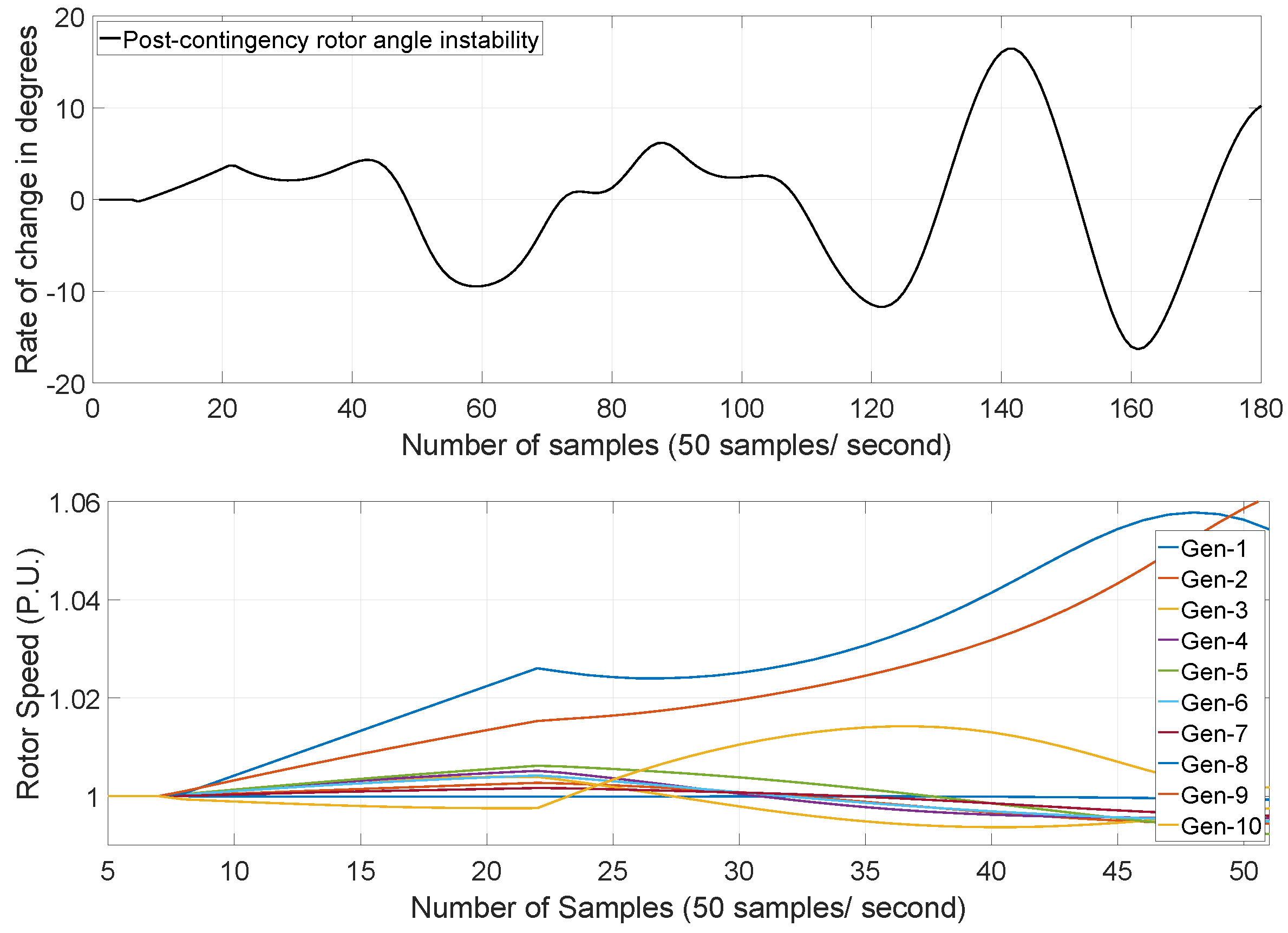
The synchronous generators in each area implement real power frequency and reactive power voltage droop control. To represent non-dispatchable energy generation, a wind power plant based on an induction generator is considered and connected in bus-36, which is closer to the Generator-7 [26]. The system considers two types of loads, critical invariant and non-critical variable load which can be shed if required. The wind power generation and the non critical loads are considered as the key stochastic parameters. The variable load is lumped in buses-8, 24, 32 [27]. In order to create a system wide rotor angle instability, a critical short circuit fault have been introduced close to the bus-16 and bus-17 [28]. It makes the generators, swing against each other in groups. The event is captured in Figure 2. The top half of Figure 2 shows the rotor angle in one of the generators, during the occurrence post fault instability. The bottom half of Figure 2 shows the generator speeds right after the short circuit fault.
The energy function dictates that if a critical disturbance occurs in the system, mechanical and electrical power go out of balance. Depending on the disturbance, the change in rotor angle may introduce a rotor angle instability. In turn, the rotor angle instability introduces large voltage fluctuation in the transmission lines. The transmission line voltage fluctuations can also be spotted from the terminal voltage of the generators affected by this instability. In this study, the terminal voltage data has been used to develop an optimized active power corrective control (CC) to eliminate the rotor angle instability in each of the islands. The corrective control parameters or the active power from different generators varies with the available wind power and load [29,30,31,32].
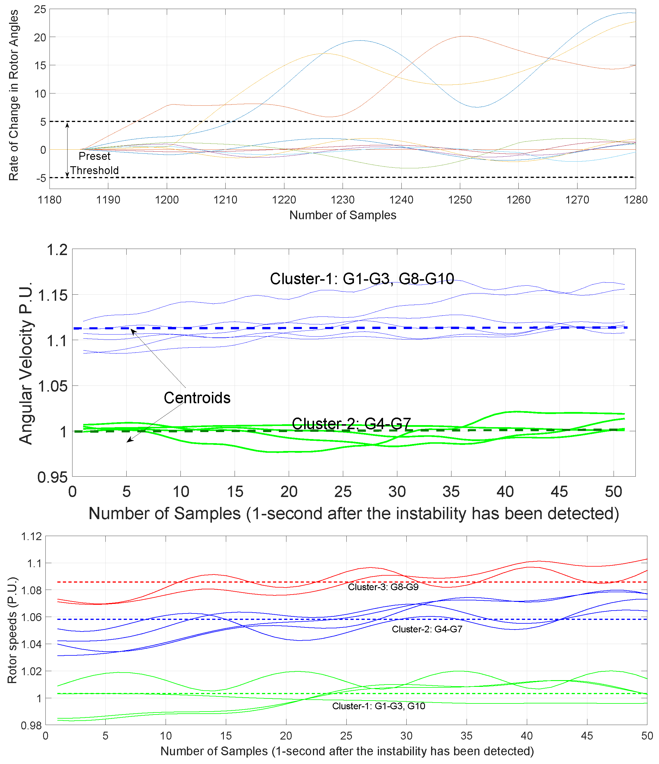
The machine learning algorithm developed is based on different power system events associated to FDIR. Within the time-line of different events, by analyzing the dynamic data collected from the generators, a distributed supervised secondary control scheme is developed; to achieve d E G d t 0 ( E G = Generator terminal voltage); after a major disturbance. The supervised secondary machine control is a process that includes the above mentioned CC technique. The proposed method is a modified and extended approach carried out in Reference [33]. The modification is brought by introducing a feature extraction method. The system is designed to have both normal operating mode and self healing mode, in this study only the self healing mode is considered. The self healing mode is invoked once a rotor angle instability is observed, right after a critical fault is cleared. After a large number of offline simulations, for this model it is observed that, the rate of change in between 5 ° / to + 5 ° / s in rotor angle deviation indicates a critical rotor angle instability where the grid has to be operated in the self-healing mode. The observation is shown in Figure 3. After 1-second or 50 samples of the fault, the breach in threshold is clearly visible in the figure.
The model in Figure 1 is used to generate time series dynamic data for training and testing the machine learning platform for the proposed supervised secondary controller. The proposed model is a modified IEEE-39 bus system, which is suitable for stability analysis. The demand and wind speed are randomly varied in order to do a Monte Carlo based simulation to prepare a stability database with the synchronous generator data. The dynamic parameters chosen are in per unit quantity and these are rotor speed ω , rotor angle deviation d δ , active power generated P E , and terminal voltage E G . For simplicity, only the cases where the system can be stabilized and restored by dividing it into two segments are considered. During any contingencies these parameters from the generator, affected nodes is collected. These parameters are timeseries in nature. During the contingency from their dynamic behaviors, patterns in form of features are extracted. For example, the magnitude of a generator terminal voltage is considered dynamic during the contingency. Feature extraction is applied on that time series data in order to develop training and testing data for the next phases. A matrix of 444,037 × 36 is developed from the nine synchronous generators. Generator-2 is considered as the reference bus for calculating d δ , therefore, the supervised control is not applied on this generator.

3. The Proposed Supervised Control

3.1. Controlled Islanding

Controlled islanding mechanism can be an effective way to mitigate system-wide instability and help restoration [25]. The method proposed in this study, applies an unsupervised machine learning algorithm on rotor-speed data in order to develop a coherency based grouping [25,34]. Power system can be modeled as a set of coupled differential algebraic equations as functions of rotor speed. Due to the nature of such coupling, rotor speed can often be used as an indicator for detecting coherent groups. An unsupervised clustering can be used as a tool to detect such groups [17]. At first, the process randomly selects centers for each cluster. The number of clusters is pre-defined. The membership of each data point is decided based on the objective function, that minimizes the Euclidean distance of each data point y i k with the corresponding centroid z i . Through this objective function the sum of all the Euclidean distances between every data point to their cluster-centroids.
D ( y i k . z i ) = k = 1 d i = 1 C ( y k z i ) 2
Here, d is the number of data points, C = 1 , 2 , 3 depending on the number of islands or no islanding required, z i is the centroid of i-th cluster and y k is the k-th data point. Once the D is calculated the centroids are re-selected and the objective function is repeated.
C i = 1 n i y p s i y p
Here C i is the center of the i-th cluster, n i is the number of data points which in this case is the rotor-speed observed within an 1-second data window after an instability is detected. y p is the data vector after p t h iteration. 1-second data window is observed to be sufficient, to detect the coherency. The group is prepared, once the three phase fault is cleared but no restoration process or islanding has been implemented yet. In the Figure 3, the clusters are shown in three colors with their centroids. In middle section of the figure it is shown that, based on the coherency observed, two sets of generators have been prepared. cluster-1 consists of {G1-G3, & G8-G10}, represents Area-1 and cluster-2 consists of {G4-G7}, represents Area-2. The areas are created by disconnecting the transmission lines between node-(16&17) and node-(14&15). Similar clustering is also shown in the bottom part of the figure, with three groups of generators. The number of clusters are selected based on the available empirical data. During the training phase the clusters are prepared based on the coherency observed.

3.2. The Corrective Control

The primary control in an isolated grid may not be sufficient as it may cause frequency deviation after a non critical fault. Therefore, the secondary control is required, which implements a slower dynamics to fine tune the control parameters and prevents the frequency fluctuations. However, under a critical fault when the system wide rotor angle instability is observed, a secondary control often fails to stabilize the system [30,31]. This study implements a machine learning driven supervised secondary control during the post fault scenarios, where secondary control cannot maintain stability after a critical fault. The supervised secondary control is considered as the topmost part of a hierarchical control scheme [19,33,35].
The conventional droop characteristics satisfies the condition D P i P N i = Δ ω m a x and D Q i Q N i = Δ E m a x [3]. Where, i is the i-th stochastic scenario, N is the number of synchronous generators, P and Q are the generated active and reactive power, Δ ω m a x and Δ E m a x are angular frequency and voltage deviations allowed. This study only considers scenarios where the allowed Δ ω m a x is exceeded. The dynamic response can be further understood through a linearization of the active and reactive power equations through a set of small signal models.
Δ P ( s ) = G s + D P G Δ ω * ( s )
Δ Q ( s ) = H 1 + D Q H Δ E * ( s )
Here, the coefficients, G and H depend on the nominal terminal voltage and the rotor angle of the generators and the transmission line voltages where power is transmitted. The secondary control scheme is evoked if the threshold of the Δ d θ m a x is crossed after a short circuit fault, as shown in Figure 3. At steady state conditions, under different stochastic scenarios, the voltage magnitudes and the angular differences between one generator and the point of common coupling is kept within a boundary by the PSS and governors. It results in a list of Δ P and Δ Q . Therefore, a Monte Carlo based simulation strategy is developed to prepare a stochastic database of the aforementioned P N i , Q N i , Δ P and Δ Q . During a rotor angle instability the supervised controller changes the active power references and keeps the active power generation fixed through the turbine governor. Due to this action the Δ ω decreases and Δ P falls within the boundary suitable for the pre-tuned PSS. The database for optimized active power reference for different stochastic scenarios, is developed using genetic algorithms [2]. Overall this process is considered as the Corrective Control (CC). The CC is based on the following objective function:
O b j e c t i v e : m i n ( ϵ V f a u l t = j = 1 M [ V p r e f a u l t V p o s t f a u l t ( i ) ] 2 ) .
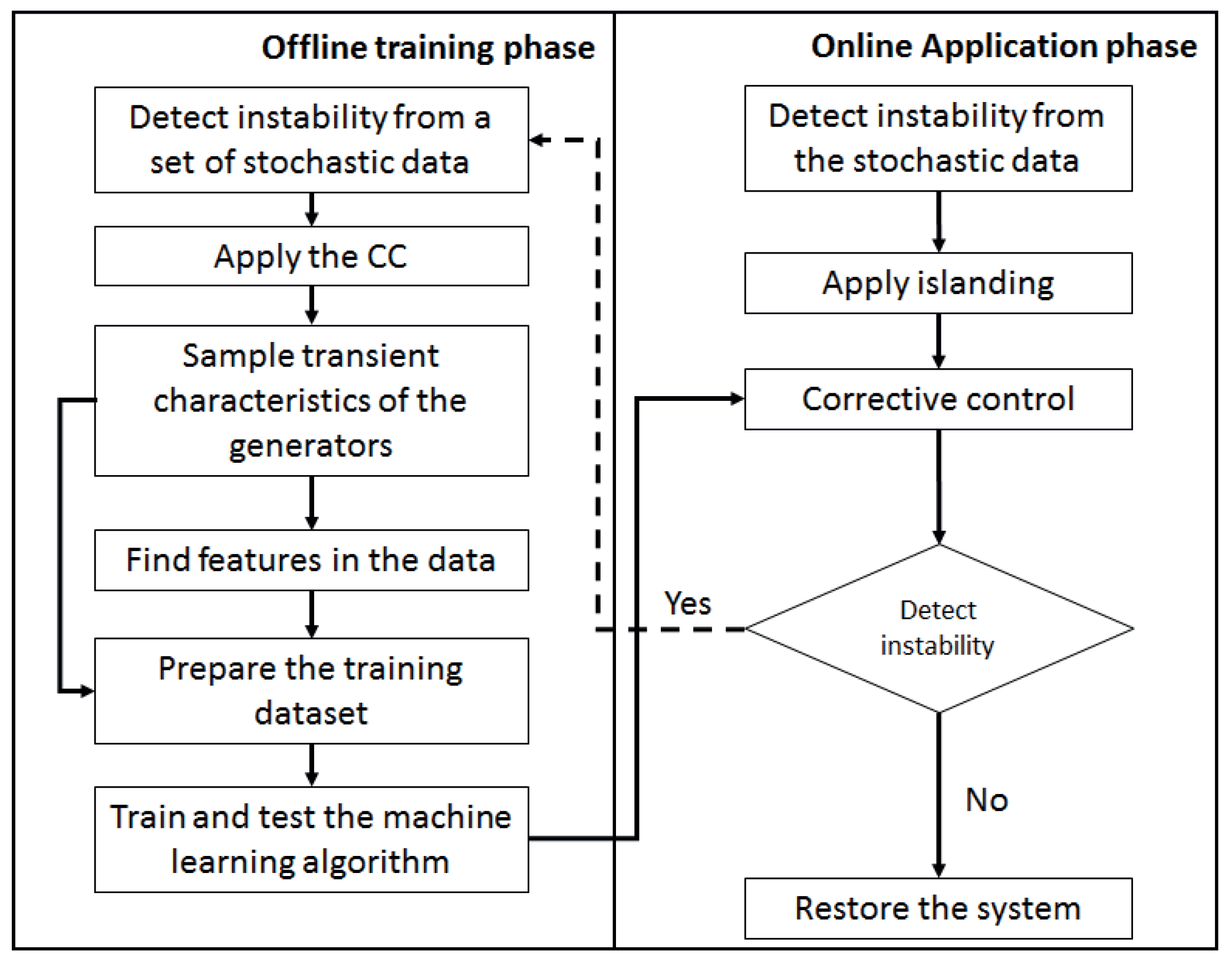
If the steady state ϵ V f a u l t ϵ t h r e s h o l d , the supervised control scheme is stopped. Here, j is the current data sample and M is the total number of data samples in that segment. For this study M = 300 equivalent to a five-second data window has been chosen. The objective function is subject to the constraint 0 P N P N , m a x , 0 P l s where, N refers to the number of synchronous generators. P l s refers to the minimum temporary load shed. The overall system load is divided into two parts, variable demand and fixed demand. The temporary load shedding is carried out from the variable demand to maintain the energy balance; i = 1 n g p g i + i = 1 n w i n d p w i n d i = P d p f l + P T l o s s + P l s . Where, P d p f c l is post fault load, P T l o s s is the transmission line loss, p w i n d i power generated from the wind power plant, n g is number of synchronous generators, n w i n d = 1 . Once the system becomes stable the load is also restored. In this study, island area-1 requires temporary load shed when the wind power is relatively high. The overall workflow for the CC based control is shown in Figure 4. The workflow is divided into two phases, offline and online. The offline phase is based on a test and trial approach. The process initially starts with different stochastic scenarios. The CC is then applied to stabilize each segment and restore the grid. The CC is an optimization technique and the dynamic data obtained from the generators after CC has been applied is used for feature selection. These features represent different events and also the optimized decision parameters under that stochastic scenario. Once the machine learning algorithm is trained, it is then used in the online phase for making decisions for the CC. Being stochastic in nature, some of the predictions yields misclassification errors. Those data are used for further training.
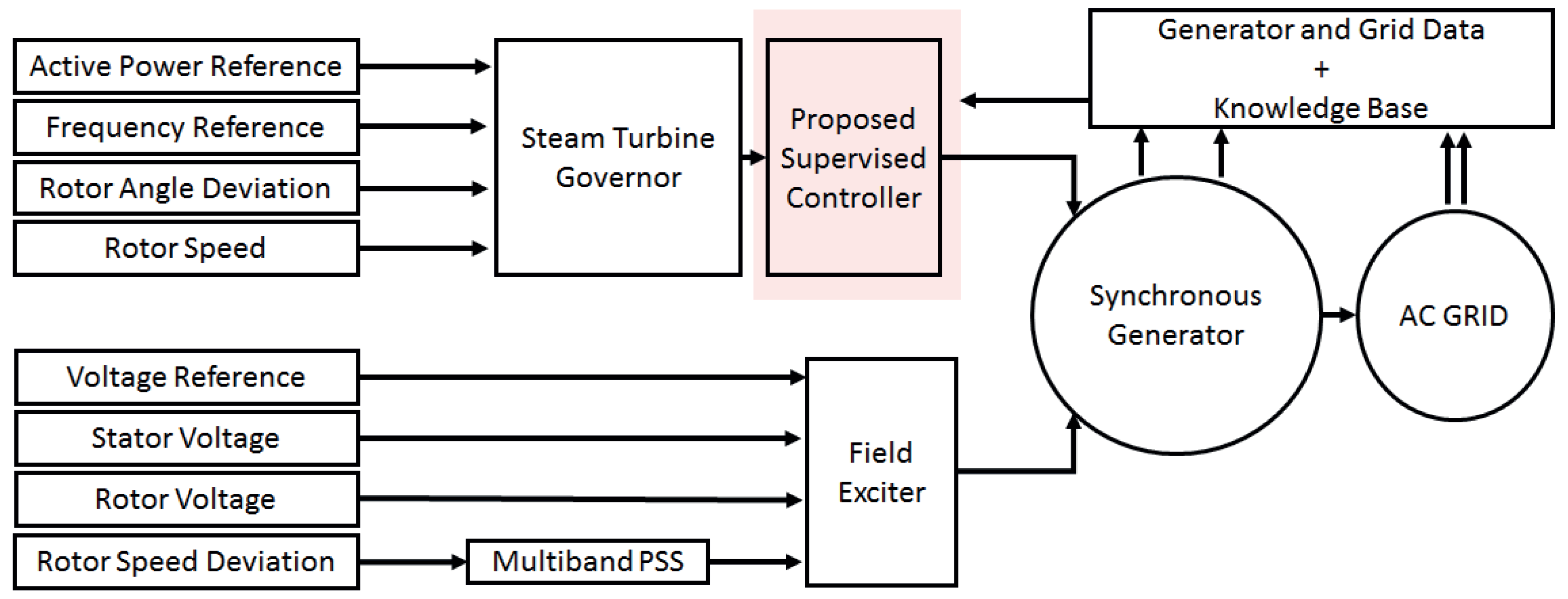
Figure 5 shows the proposed model of the secondary control system. The supervised control is based on machine learning algorithms trained under different stochastic scenarios on the feature data to perform the proposed corrective control (CC) followed by islanding. The features are introduced in the consequent sections.

3.3. Power System Events

Based on different wind power, loads, fault locations and number of faults; several cases have been observed. In each of these cases one or multiple critical three phase faults and consequently system wide rotor angle instability have been introduced. Based on these criteria the system has been either divided into two, three islands or no island at all. Table 1 shows a list of probable contingencies leading to three different islanding schemes.
Each of these cases has further been divided into multiple events namely, Fault, Post fault rotor angle instability, Supervised control and Post restoration. If the proposed system, fails to restore the grid, then the scenario-data is fed back to the offline training stage.
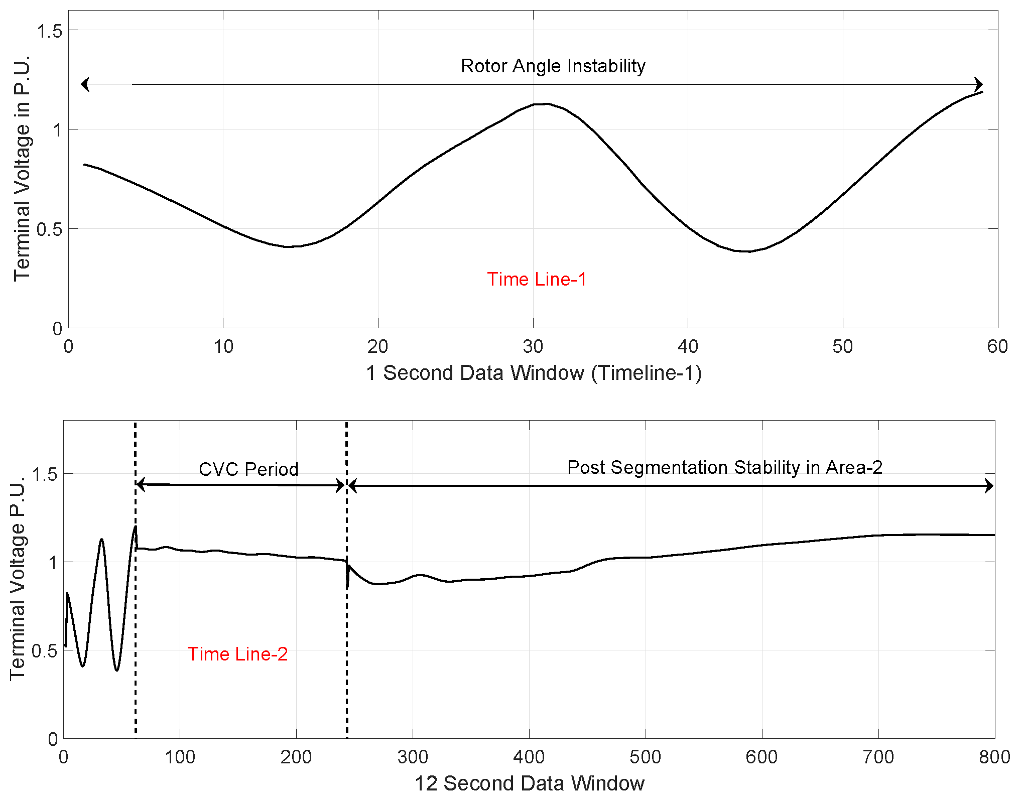
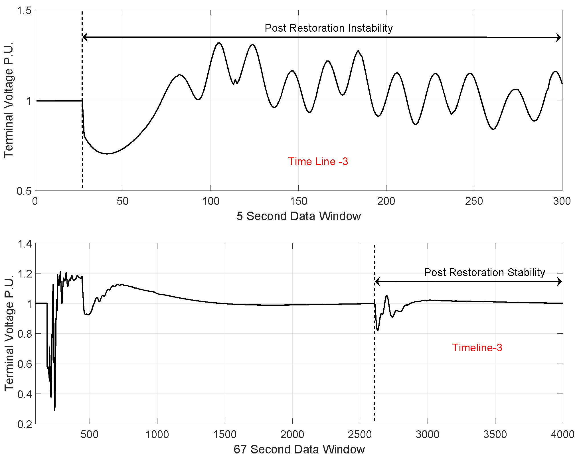
From the four above scenarios three time-lines are chosen, time-line for detecting post fault rotor angle instability, time-line for CC to stabilize the islanded network, and time-line representing the post restoration period. The two latter periods can either be stable or unstable. In Figure 6, all the different time-lines have been shown. Time-line-1 data is the candidate for decision making, time-line-2 is for applying CC and time-line-3 is the candidate data for evaluating the performance of the algorithm. Here, for a better understanding, terminal voltage of generator-7 has been chosen to demonstrate the events.
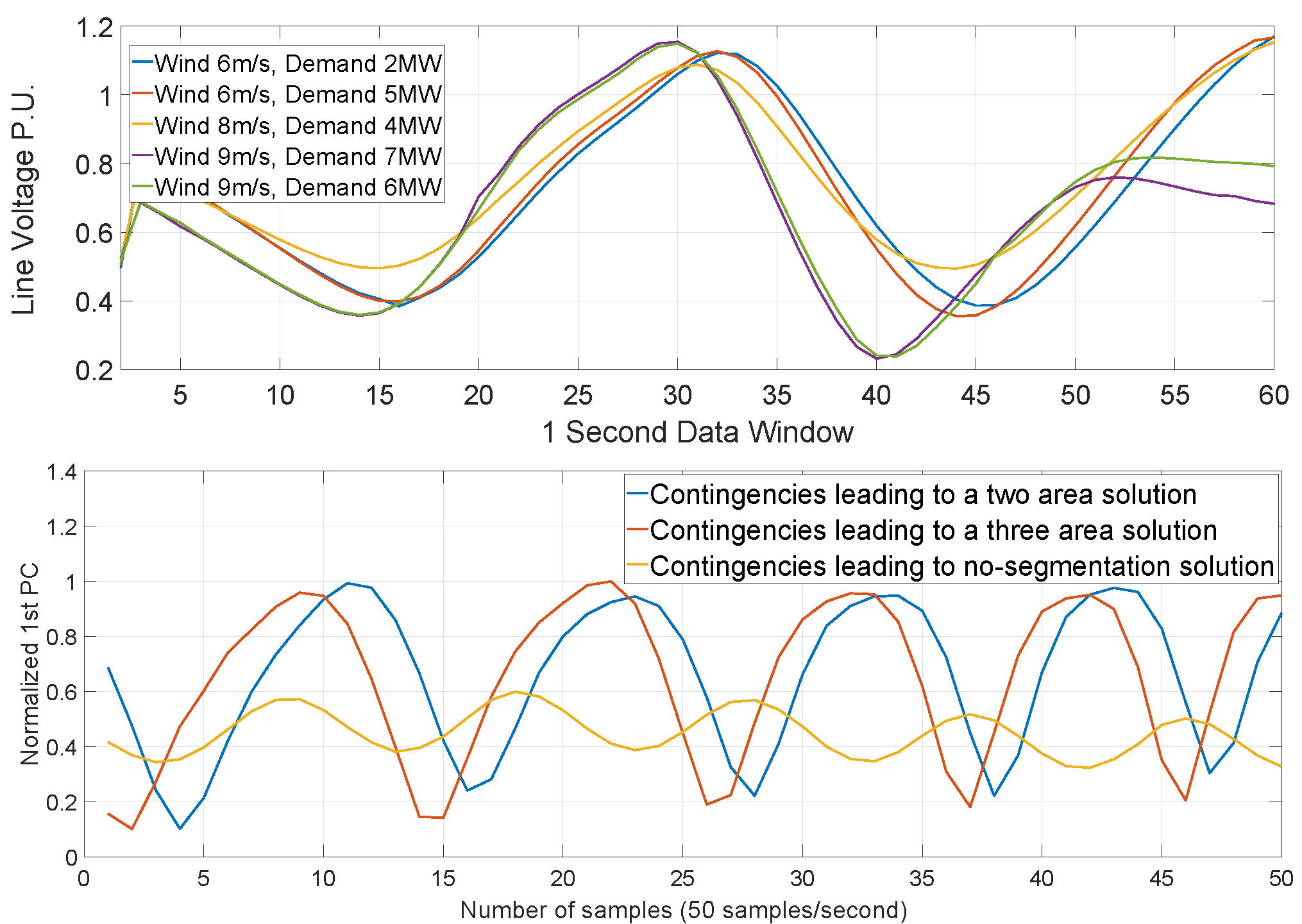
Furthermore, Figure 7 shows an example of the terminal voltage at Generator-7 under different scenarios (wind power and load), during the rotor angle instability. The similarity in the time series data is overwhelming, and that makes the application of a machine learning algorithm quite difficult [36]. However, each scenario has its own events and therefore, features can be used for distinguishing those events in each scenario.
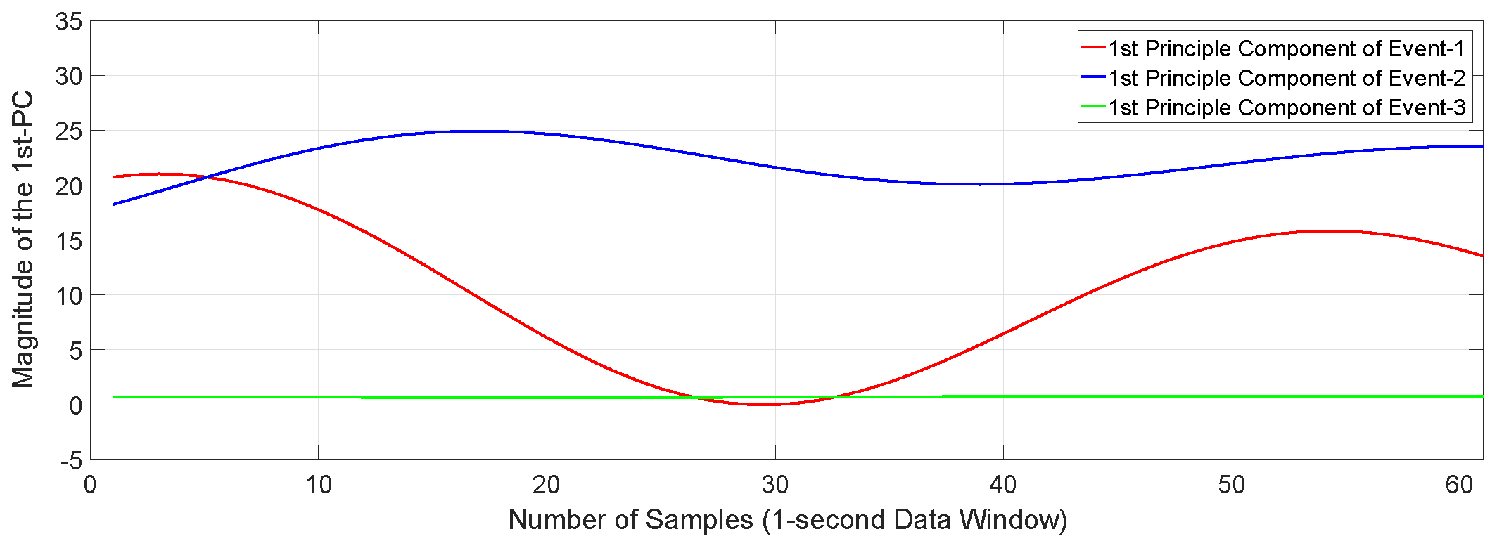
Like Figure 7, a similar variation in the phasor-signals is also observed in rotor speed and rotor angle from each synchronous generator. Such similarities in data makes it difficult to select a candidate for feature selection. Therefore, to retain information that can be crucial for the feature selection process, principle component analysis is carried out on these three types of phasor time series data [6]. The Principle Component Analysis (PCA) finds out the first component accounted for the most of the variations in generator data matrix. The variability is around 75%. The data matrix X has m number of observations with n = 3 number of attributes. The m-number of orthonormal basis functions are represented by W which is of n n dimensions. The data matrix is then represented as X = T W , where T is ( t 1 , i . . . . . t m , i ) , which is used to form the coherent clusters for identifying principle components. Figure 8 shows that a significant variation in signal magnitudes and widths can be spotted in the reduced data (1st principle component) among different events. It further justifies that, the use of PCA for reducing the generator data and using that data for extracting features, is meaningful.

3.4. Available Observed Features

As shown in Figure 8, the principle components have unique distinction in their shapes under different events. However, due to the nature of time series data, overlapping magnitudes confuses the learner. One solution is to use a large dataset for training. On the other hand this problem can significantly be overcome with the use of features [14,37]. Base on the discussion presented in earlier section, in this study three features, distinguishing each event, have been chosen. The selection process is mostly inspired by the observed variations in magnitude. Another motivation is drawn from the fact that, the inherent properties of a power system can provide significant information on a set of dependent variables based on a set of argument variables. This understanding is quite effective in detecting online phenomenon such as sensitivity. For example, active power can be used as a dependent-variable and node-voltage can be used as argument-variable to understand the voltage stability of a system [1]. Therefore, sensitivity data holds useful information. Moreover, feature extraction is a computationally expensive mechanism [37]. Thus, a set of simple and predefined features based on domain knowledge can reduce the computation burden. Keeping these issues in mind, this study selects the following three features:
  • Prominence of local maxima in terminal voltage [38,39,40]
  • Available frequencies in the time series voltage data [41]
  • Sensitivity P E / V f . Where, V f is the voltage at the fault bus and P E is the active power generation from the subject generator [16].
Event detection and decision-making based on time-series data is not a predictive, rather a prescriptive analysis. In order to associate a feature with the underlying events in the time series data, a frame of reference has to be used. In this study the frame of reference is developed by using a sliding window technique on the time series data and recording the features. To do so, a 1-second transition-window is selected to extract features and then those features are converted to different ‘factors.’ By ‘factors’ this study refers to a quantity that can represent a window using only one number. This action is necessary to represent the sliding windows using row vectors. After calculation, those factors are stored in the data-table. As mentioned earlier, each row signifies one attribute window. This table is later used to train the machine learning algorithm.
To prepare the features in each data window, sixty samples per second have been considered. The variation in magnitude of the first principle component has been considered as the first feature. The method followed here is inspired by Reference [40]. A normalized window of 1-second duration in the time series data is chosen to carry out the feature extraction.
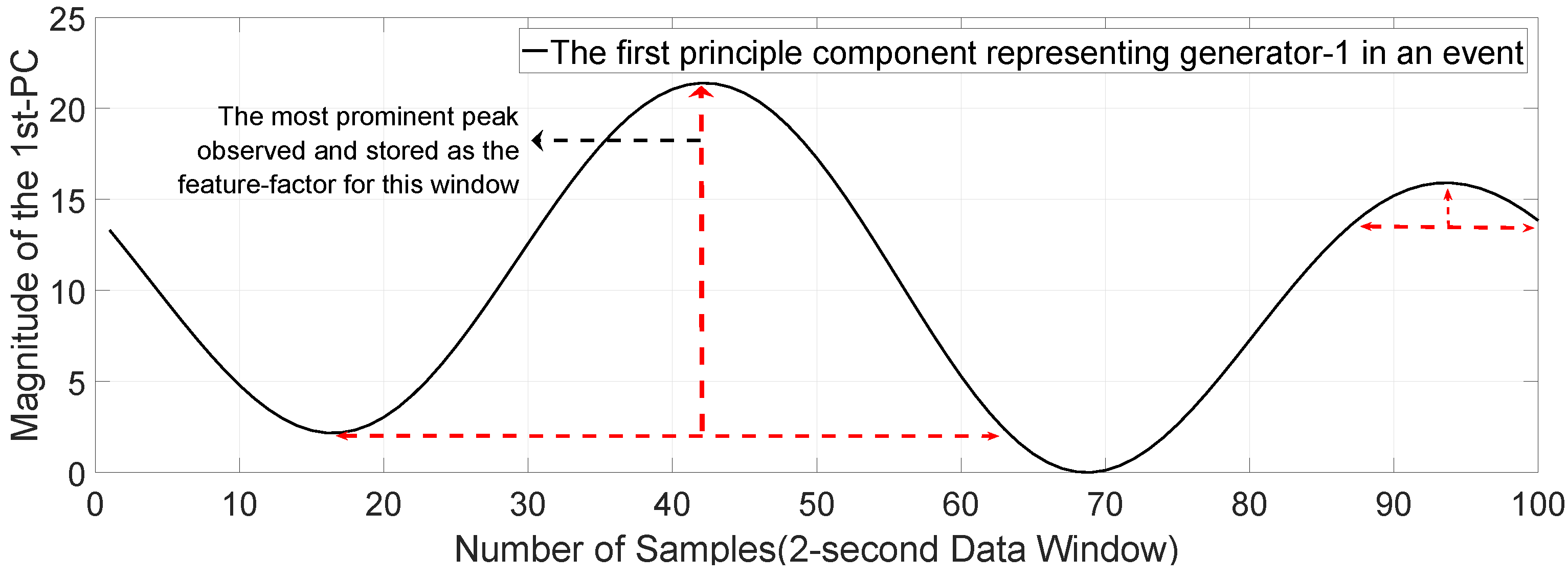
First, a lowest contour line in the 1-second data window circulating a local maximum point has been detected. Then the height of that point is measured and a ratio is prepared in terms of that contour line. Figure 9 shows the method of finding prominent local maxima from a normalized window of the principle component of one of the generators. For clarity of vision a 2-second data window is selected for Figure 9. Once several prominent peaks are detected, the maximum available prominent peak is considered as a feature-factor for that data window and stored in the training data table.
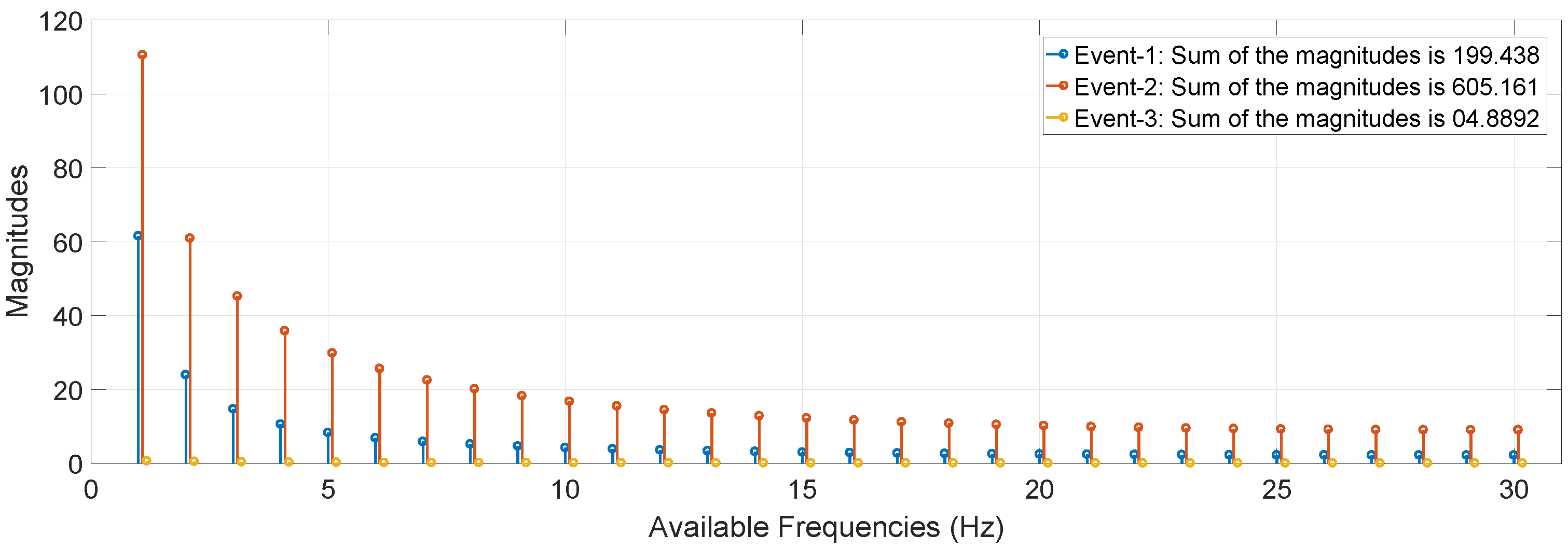
The second feature is based on the available frequencies in the first principle component, observed in the 1-second data window. This feature is extracted through a Discrete Fourier Transformation (DFT) technique; x [ n ] = n = 0 N 1 1 N X ˜ [ k ] e j k ( 2 π / N ) / n , K = 0 , 1 , . . . . N 1 . Here, X ˜ [ k ] is the amplitudes and x [ n ] is the linear combination of the complex exponentials with that amplitude. Decision making based on frequency data has often been observed in the field of harmonics and power quality analysis [41]. In this study, a frequency spectrum of the first 30 Hz has been chosen as the featured attribute as shown in Figure 10 (with a small displacement in the X-axis for the purpose of visualization). As the sampling rate used in this study is 50 samples/seconds, according to the so called ‘Nyquist-theorem’ DFT can observe upto 30 Hz. Once the magnitudes of those frequencies are calculated, the magnitudes are summed up to be used as a feature-factor for that data window, i = 1 30 M i . It is called a frequency factor.
A sensitivity data, based on the voltage at fault bus and the active power generation from the subject generator is considered as the third feature [1].
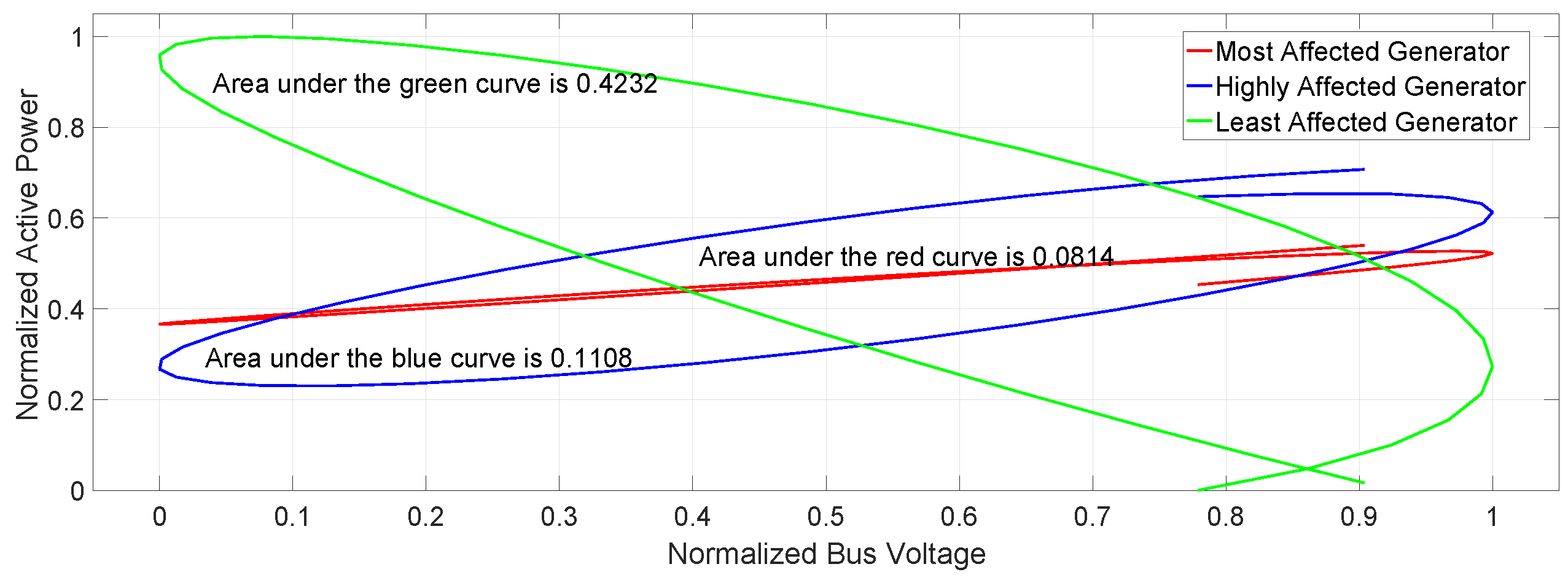
In Figure 11, which is inspired by Liapunov’s direct method, three sensitivity curves of the generators {G7, G1, G8} are shown in terms of the fault bus voltage at bus-16. It clearly shows the aperture of the curve varies depending on the impact of fault. The figure refers to the idea that, less sensitive relations have a larger aperture. To calculate the aperture, trapezoid method of numerical integration is used. The limit of each response curve is considered between two extreme points over the X-axis or the Δ V f b u s axis. Two extreme points develops a convex (Upper) and a concave (Lower) perimeters. Then the area under the curves are calculated. The overall area of the aperture is then assumed by subtracting the area under the concave curve from the convex; A r e a = A c o n v e x A c o n c a v e . This area of aperture is then used as the feature-factor that represents the data window.
V 1 V 2 f ( x c o n v e x ) d x V 2 V 1 2 N n = 1 N ( f ( x n ) + f ( x n + 1 ) )
V 1 V 2 f ( x c o n c a v e ) d x V 2 V 1 2 N n = 1 N ( f ( x n ) + f ( x n + 1 ) ) .
Once the training data-table is prepared, it is used to train a multiclass classifier. Overall, the training process only considers data that ensures system stability. It means the classification algorithm is trained based on the concept of resiliency. The decisions leading towards post fault stability that returns to pre-contingent state are considered accurate decisions.

3.5. Multiclass Classifier

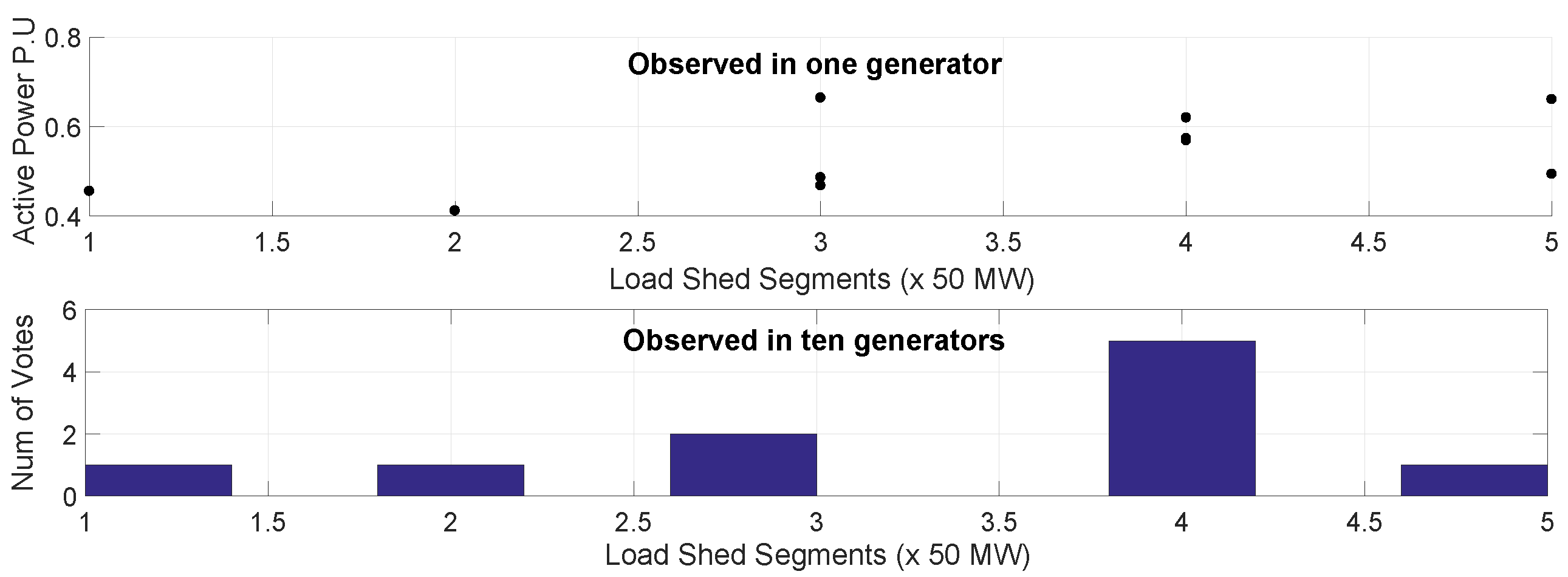
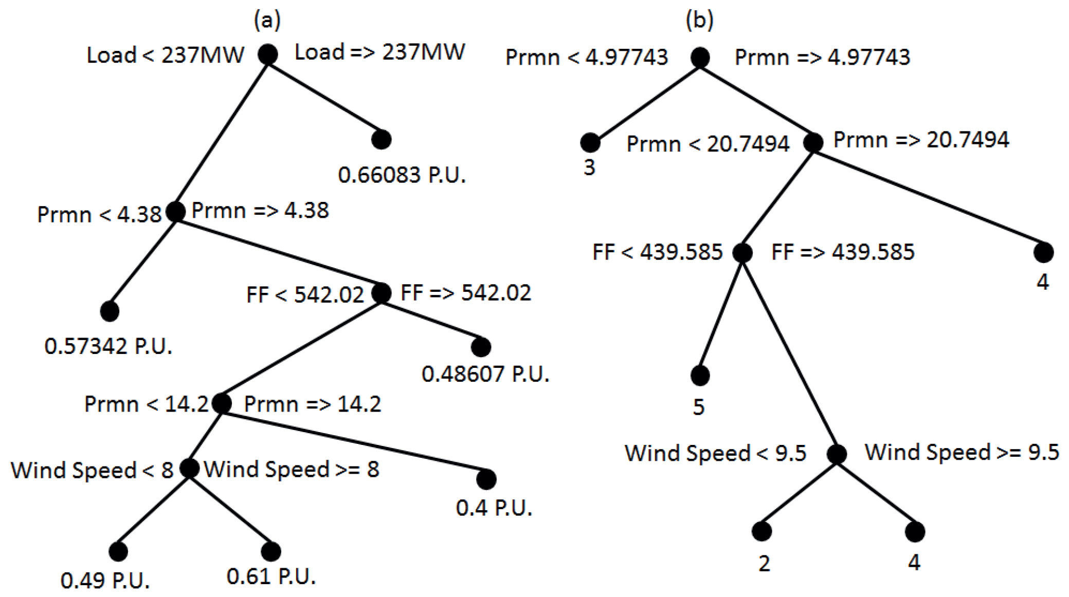
The chosen Multiclass classifier is an ensemble of bagged decision trees trained using the stochastic parameters and the features. The bagged decision trees weigh and reweigh the predictor variables and their estimates. For example; a function estimate g ^ e n s = k = 1 M c k g ^ k ( . ) is obtained based on the k t h reweighed data with the combined linear estimation co-efficient c k . This method is deployed to eliminate classification error due to estimation variance and also statistical bias, specially in a stochastic scenario [32,42]. The ensemble method implemented in this study is prepared using one hundred fully grown trees by splitting the attribute data into one hundred training sets, D 1 , D 2 , …, D 100 . This approach helps to obtain an improved composite model. M i ( 1 i 100 ) classifiers vote by predicting a class and the ensemble selects the final class from those votes. The overall technique along with Random Forest and Random Subspace also includes Bagging and Boosting [36]. Depending on the number of controlled islands observed in each contingency, different values of the features are obtained. Three separate tables Table 2, Table 3 and Table 4 are shown below based on the number of islands. Each table shows the attributes wind speed, Variable Demand, Snsvt which is the feature-factor derived after sensitivity analysis, Prmn is the prominent maximam peak obtained from the principle component, FF is the frequency-factor derived from the DFT of the principle component. The tables are prepared from the data collected from generator-4. The classifier has a target attribute named Decisions. The decisions are combination of active power reference (0-1 P.U.) for the governor of the generator and the amount of temporary load shedding required in the Area-1. Both the information has been collected from the offline simulation after conducting the CC on each of the generators. n-number of decision combinations are observed and it is different for different generators, for example, for a two-area solution; in case of generator-1 n = 4 and for generators-4&7 n = 7 . The control parameters are unique for each generator however the amount of load shedding required in each scenario is considered through a voting based on statistical mode [2]. To synchronize the voting process the load required to be shed is represented as segments of 100 M W , 200 M W , 300 M W up to 500 M W . An example of the decisions is shown in Figure 12. The upper figure shows the combination of two parameters observed in the decisions in a generator. The figure shows how the voting process and the active power reference are related in one generator under multiple scenarios. Both the estimations are carried out by the multiclass classifiers placed in each generating stations. The lower figure shows an instance of the voting process from the 10 synchronous machines in one scenario. As segment-4 got the maximum vote 4 × 100 M W load is temporarily shed from the Area-1.
The decision trees, prepared from the above mentioned method, are shown in Figure 13 with a small example data set. The upper tree shows the decisions for selecting the amount of load shedding required in Area-1 . Data of the right tree is collected from all the synchronous generators and is used for the voting process for the purpose of load shedding, as shown in Figure 12. The left tree shows the active power reference set in that generator. The trees are prepared using generator-4 and time-line-1 data.
The classification accuracy is measured against the system resiliency during low probability high disruptive events. If the classification algorithm can predict decisions that lead towards a stable pre-contingent state the algorithm is considered to be accurate.

4. Results

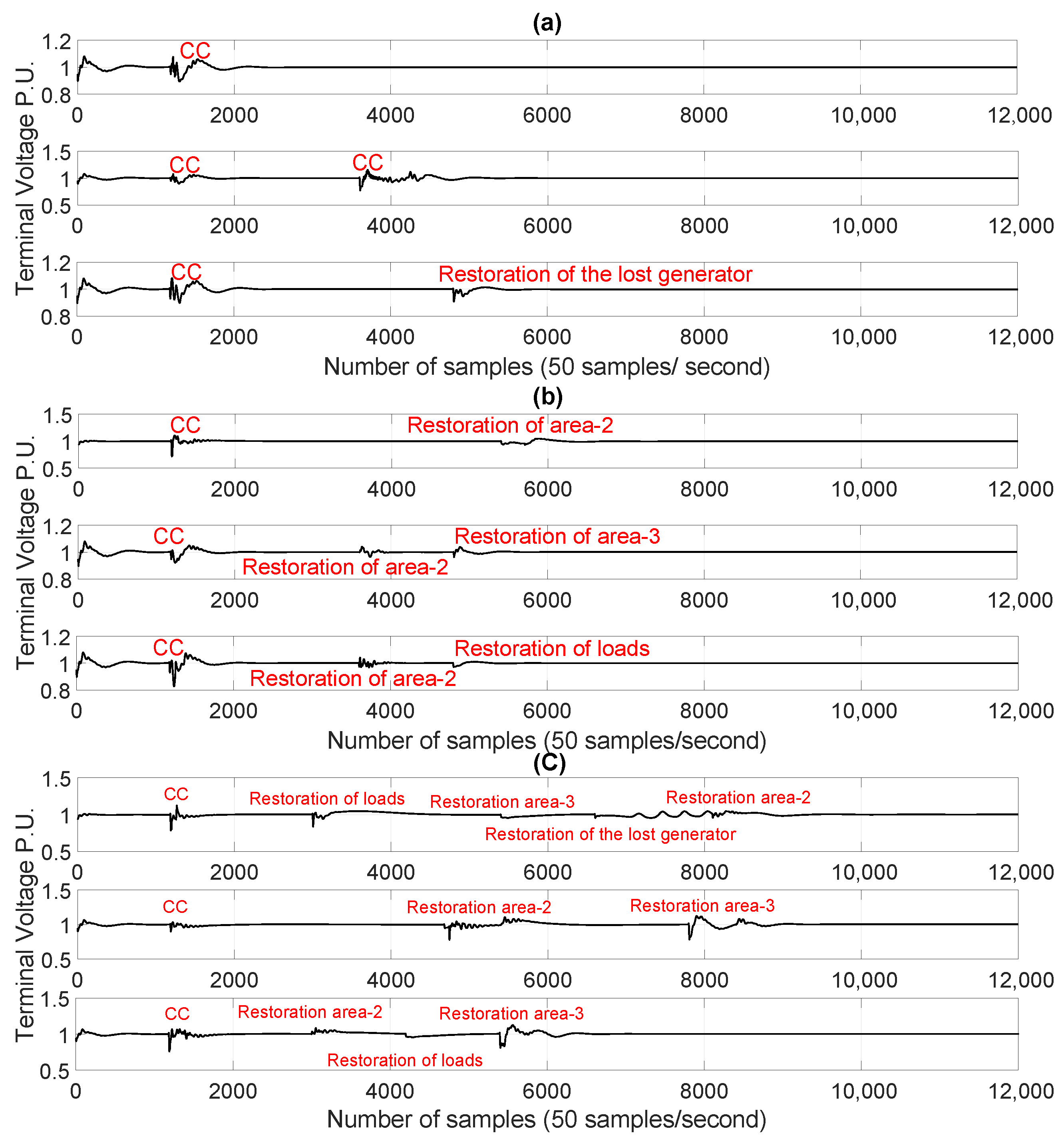
Figure 14 shows three scenarios of the three proposed solutions under multiple contingencies and operational decisions as explained in the earlier sections. One interesting observation can be made that, in different stochastic scenarios the duration as well as the sequences of the timelines vary, specially for the scenarios where multiple faults lead towards a three area solution. The system resiliency is considered based on the post restoration terminal voltages. If the consumers are restored and the system voltage remains stable, the algorithm is considered to be improving resiliency.
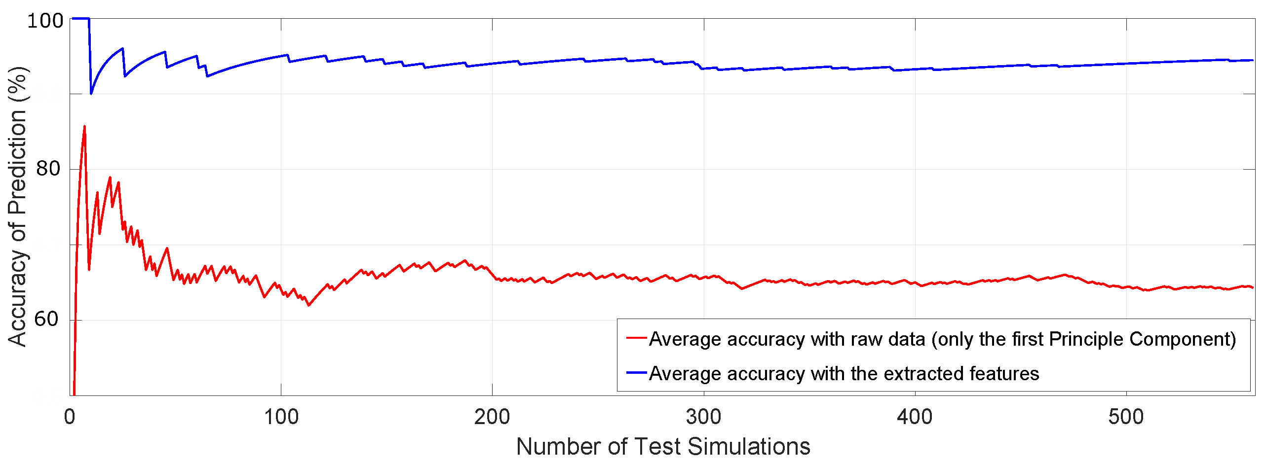
Each of these time-lines has been assessed using Monte Carlo based simulation strategy by randomly generating wind power and demand. Based on these randomly selected stochastic scenarios, n i decisions have been identified in this study, where n i means n combination of decisions for the i-th generator. These decisions can maintain a post restoration stability. For example; for the two-area based solution, the Monte Carlo based simulation is carried out for a limited 1560 scenarios. Where, 1000 scenarios have been used for training the algorithm and rest of the 560 scenarios have been used for testing. Figure 15 shows a comparison of the average prediction accuracy between the proposed method with features as well as the prediction without features. Only the first principle component has been used as raw data where no feature has been extracted. If the system is completely restored the accuracy is considered ‘1’ else ‘0’. The overall performance shows around 95 % prediction accuracy with the features. With a limited 1000 scenarios, feature data has been proven to be quite helpful to reach such high degree of accuracy. The proposed accuracy is also a marker for symbolizing system resiliency. If the therefore, 95 % accuracy also refers that in 95 % cases the system remains resilient.
The rest of the 5 % cases where the algorithm misclassified the decisions, the system recovery could not be achieved. Once the areas are restored through the transmission line the overall system became unstable.
The proposed algorithm has also been compared with the similar methods proposed for the purpose of power system event detection in the previous literature [10,17]. Table 5, shows the comparison of accuracies in identifying ‘timeline-1’ under three different scenarios. The three scenarios are randomly selected among three-area solutions, two-area solutions and the no-segmentation solutions. Due to having additional information in the form of features, the proposed algorithm is demonstrating superiority. Figure 7 can be brought as a point of reference for explaining such performance. The overlapping magnitudes of the principle components, makes it difficult to trace out a linearized distinction between different events. The features introduces that linearity in data segmentation for the decision trees.
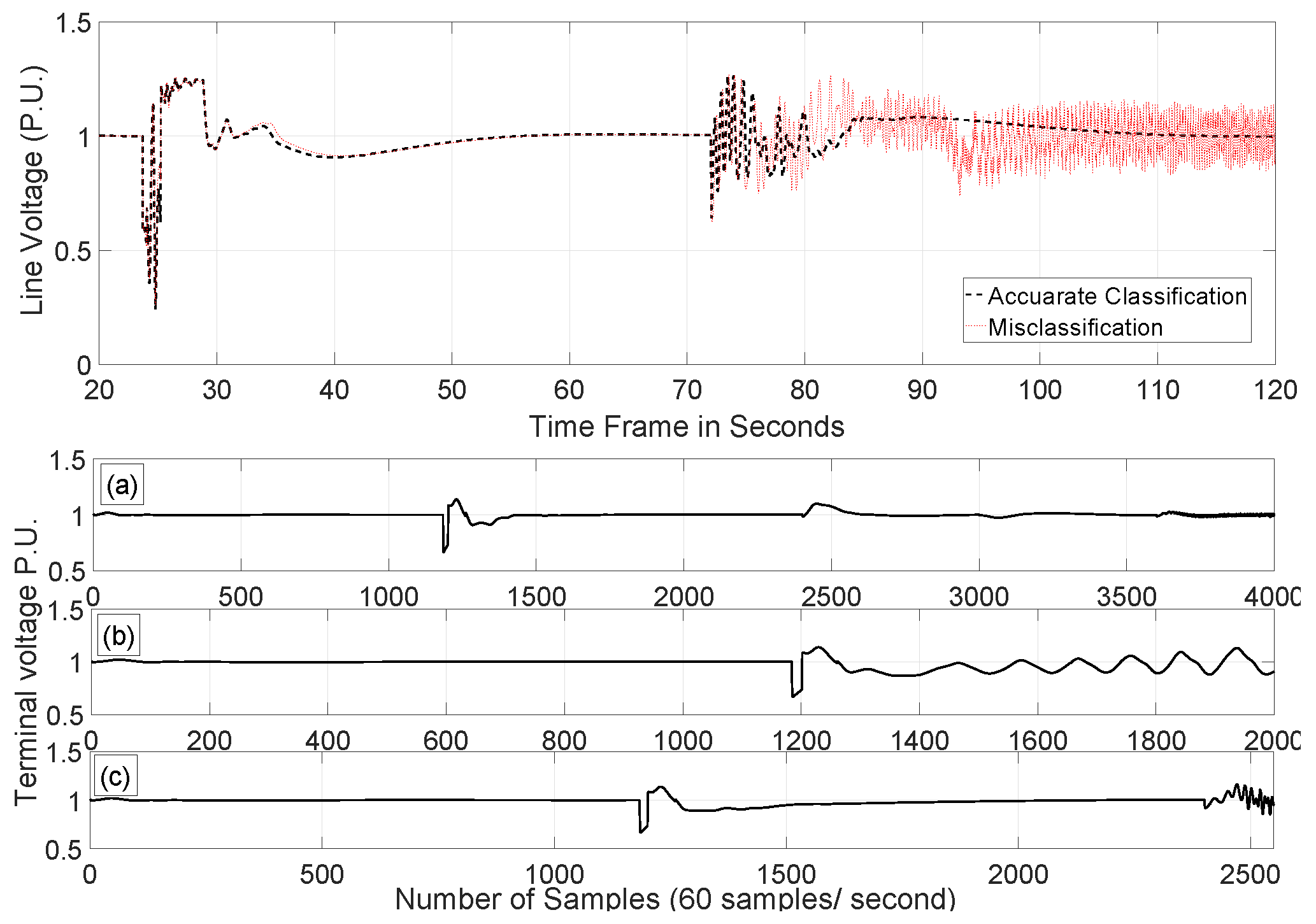
The ramifications of voting for load shed has also been speculated. It has been observed that, if the required load shedding is not carried out the system could not be fully restored. Figure 16 shows a comparison between these cases. In the top figure a comparison is shown, where in one scenario the algorithm successfully identified the right decision and in the next the algorithm could not. In the lower half of the figure, three incidents are shown where the load shedding is not carried out based on the majority voting. In each of these cases the system has moved back towards instability.
In the Figure 14, Figure 15 and Figure 16 the superiority of the proposed method can be observed. One critical observation regarding the scenarios having multiple faults is that, only the faults occurring simultaneously have been considered. In future studies different times of fault-occurrence can be analyzed.

5. Conclusions

The proposed method to predict suitable decisions for post fault restoration, has shown promising results. The method works with high accuracy despite limited number of training data has been provided. IEEE-39 bus test system, which is a large enough dynamic system, has been used to demonstrate the capabilities of the proposed method. Furthermore, the proposed algorithm is tested with high degree of stochastic influence in the network. This study is highly significant for a stand alone system where multi-machine dynamics can be observed. Based on the data analysis carried out in this study it can be concluded that, simplified features based on domain knowledge can be highly effective for the purpose of service restoration.
One critical observation is that, with an increased number of faults, the system needs to be divided into more than two areas. Under those cases the proposed algorithm heavily relies on the number of training data set provided. It is because, the optimization process in this case has to consider the sequence of operations. Thus, in case of new data sets with multiple fault scenarios, the accuracy of the algorithm decreases compare to those of the single contingency scenarios. In the author’s future experiments, the role of a centralized control scheme to address the problem of sequence control would be analyzed and compared with the proposed distributed method. Overall it can be stated that, the proposed method is showing significant promise in the filed of grid restoration techniques.
The algorithm is tested online basis. However, it is not tested on a real-time platform. Therefore, the time consumption for the decision making process varies case by case. In future studies it would be more comprehensive to apply the method on a real-time platform to address time-consumption by the system and its impact on a real-time decision-making process.

Author Contributions

M.A.K. proposed the approach, contributed in literature review, modelling, simulation, test study and in the manuscript write-up. J.C. and T.-T.L. contributed in critical review and in proofreading of the manuscript. All authors have read and agreed to the published version of the manuscript.

Funding

This research received no external funding.

Conflicts of Interest

The authors declare no conflict of interest.

References

  1. Zhang, J.; Zheng, X.; Wang, Z.; Guan, L.; Chung, C.Y. Power System Sensitivity Identification 2014;Inherent System Properties and Data Quality. IEEE Trans. Power Syst. 2017, 32, 2756–2766. [Google Scholar] [CrossRef]
  2. Al Karim, M.; Currie, J.; Lie, T.T. A machine learning based optimized energy dispatching scheme for restoring a hybrid microgrid. Electr. Power Syst. Res. 2018, 155, 206–215. [Google Scholar] [CrossRef] [Green Version]
  3. Shahnia, F.; Chandrasena, R.P.S.; Rajakaruna, S.; Ghosh, A. Primary control level of parallel distributed energy resources converters in system of multiple interconnected autonomous microgrids within self-healing networks. IET Gener. Transm. Distrib. 2014, 8, 203–222. [Google Scholar] [CrossRef]
  4. Konstantelos, I.; Jamgotchian, G.; Tindemans, S.H.; Duchesne, P.; Cole, S.; Merckx, C.; Strbac, G.; Panciatici, P. Implementation of a Massively Parallel Dynamic Security Assessment Platform for Large-Scale Grids. IEEE Trans. Smart Grid 2017, 8, 1417–1426. [Google Scholar] [CrossRef] [Green Version]
  5. Zidan, A.; Khairalla, M.; Abdrabou, A.M.; Khalifa, T.; Shaban, K.; Abdrabou, A.; Shatshat, R.E.; Gaouda, A.M. Fault Detection, Isolation, and Service Restoration in Distribution Systems: State-of-the-Art and Future Trends. IEEE Trans. Smart Grid 2017, PP, 1–16. [Google Scholar] [CrossRef]
  6. Zhou, Y.; Arghandeh, R.; Konstantakopoulos, I.; Abdullah, S.; von Meier, A.; Spanos, C.J. Abnormal event detection with high resolution micro-PMU data. In Proceedings of the 2016 Power Systems Computation Conference (PSCC), Genoa, Italy, 20–24 June 2016; pp. 1–7. [Google Scholar] [CrossRef] [Green Version]
  7. Jin, S.; Huang, Z.; Diao, R.; Wu, D.; Chen, Y. Comparative Implementation of High Performance Computing for Power System Dynamic Simulations. IEEE Trans. Smart Grid 2017, 8, 1387–1395. [Google Scholar] [CrossRef]
  8. Khaitan, S.K. A survey of high-performance computing approaches in power systems. In Proceedings of the 2016 IEEE Power and Energy Society General Meeting (PESGM), Boston, MA, USA, 17–21 July 2016; pp. 1–5. [Google Scholar] [CrossRef]
  9. Vasconcelos, M.H.; Carvalho, L.M.; Meirinhos, J.; Omont, N.; Gambier-Morel, P.; Jamgotchian, G.; Cirio, D.; Ciapessoni, E.; Pitto, A.; Konstantelos, I.; et al. Online security assessment with load and renewable generation uncertainty: The iTesla project approach. In Proceedings of the 2016 International Conference on Probabilistic Methods Applied to Power Systems (PMAPS), Beijing, China, 16–20 October 2016; pp. 1–8. [Google Scholar] [CrossRef] [Green Version]
  10. Chen, Y.; Xie, L.; Kumar, P.R. Power system event classification via dimensionality reduction of synchrophasor data. In Proceedings of the 2014 IEEE 8th Sensor Array and Multichannel Signal Processing Workshop (SAM), A Coruna, Spain, 22–25 June 2014; pp. 57–60. [Google Scholar] [CrossRef]
  11. Mohammadi, M.; Gharehpetian, G.B. Application of core vector machines for on-line voltage security assessment using a decisiontree-based feature selection algorithm. IET Gener. Transm. Distrib. 2009, 3, 701–712. [Google Scholar] [CrossRef]
  12. Jain, A.; Zongker, D. Feature selection: Evaluation, application, and small sample performance. IEEE Trans. Pattern Anal. Mach. Intell. 1997, 19, 153–158. [Google Scholar] [CrossRef] [Green Version]
  13. Niazi, K.; Arora, C.; Surana, S. Power system security evaluation using ANN: Feature selection using divergence. Electr. Power Syst. Res. 2004, 69, 161–167. [Google Scholar] [CrossRef]
  14. Geeganage, J.; Annakkage, U.D.; Weekes, T.; Archer, B.A. Application of Energy-Based Power System Features for Dynamic Security Assessment. IEEE Trans. Power Syst. 2015, 30, 1957–1965. [Google Scholar] [CrossRef] [Green Version]
  15. Abedinia, O.; Amjady, N.; Zareipour, H. A New Feature Selection Technique for Load and Price Forecast of Electrical Power Systems. IEEE Trans. Power Syst. 2017, 32, 62–74. [Google Scholar] [CrossRef]
  16. dos Santos, A.; de Barros, M.T.C. Sensitivity of voltage sags to network failure rate improvement. In Proceedings of the 2016 Power Systems Computation Conference (PSCC), Genoa, Italy, 20–24 June 2016; pp. 1–7. [Google Scholar] [CrossRef]
  17. Papadopoulos, P.N.; Guo, T.; Milanović, J.V. Probabilistic Framework for Online Identification of Dynamic Behavior of Power Systems With Renewable Generation. IEEE Trans. Power Syst. 2018, 33, 45–54. [Google Scholar] [CrossRef]
  18. Athay, T.; Podmore, R.; Virmani, S. A Practical Method for the Direct Analysis of Transient Stability. IEEE Trans. Power Appar. Syst. 1979, PAS-98, 573–584. [Google Scholar] [CrossRef]
  19. Bidram, A.; Davoudi, A. Hierarchical structure of microgrids control system. Smart Grid IEEE Trans. 2012, 3, 1963–1976. [Google Scholar] [CrossRef]
  20. Arunagirinathan, P.; Abdelsalam, H.A.; Venayagamoorthy, G.K. Remote power system stabilizer tuning using synchrophasor data. In Proceedings of the 2014 IEEE Symposium on Computational Intelligence Applications in Smart Grid (CIASG), Orlando, FL, USA, 9–12 December 2014; pp. 1–7. [Google Scholar] [CrossRef]
  21. Grondin, R.; Kamwa, I.; Trudel, G.; Gerin-Lajoie, L.; Taborda, J. Modeling and closed-loop validation of a new PSS concept, the multi-band PSS. In Proceedings of the 2003 IEEE Power Engineering Society General Meeting (IEEE Cat. No.03CH37491), Toronto, ON, Canada, 13–17 July 2003; Volume 3, p. 1809. [Google Scholar] [CrossRef]
  22. Lee, D. Ieee recommended practice for excitation system models for power system stability studies (ieee std 421.5-1992). Energy Dev. Power Gener. Comm. Power Eng. Soc. 1992, 95, 96. [Google Scholar]
  23. Grondin, R.; Kamwa, I.; Soulieres, L.; Potvin, J.; Champagne, R. An approach to PSS design for transient stability improvement through supplementary damping of the common low-frequency. IEEE Trans. Power Syst. 1993, 8, 954–963. [Google Scholar] [CrossRef]
  24. Liu, D.; Antsaklis, P.J. Stability and Control of Dynamical Systems with Applications: A Tribute to Anthony N. Michel; Springer Science & Business Media: Berlin, Germany, 2012. [Google Scholar]
  25. Teymouri, F.; Amraee, T.; Saberi, H.; Capitanescu, F. Towards Controlled Islanding for Enhancing Power Grid Resilience Considering Frequency Stability Constraints. IEEE Trans. Smart Grid 2017, 10, 1735–1746. [Google Scholar] [CrossRef]
  26. Rabiee, A.; Soroudi, A.; Keane, A. Risk-Averse Preventive Voltage Control of AC/DC Power Systems Including Wind Power Generation. IEEE Trans. Sustain. Energy 2015, 6, 1494–1505. [Google Scholar] [CrossRef]
  27. Babazadeh, M.; Karimi, H. Robust decentralized control for islanded operation of a microgrid. In Proceedings of the 2011 IEEE Power and Energy Society General Meeting, Detroit, MI, USA, 24–28 July 2011; pp. 1–8. [Google Scholar] [CrossRef]
  28. Vittal, E.; O’Malley, M.; Keane, A. Rotor angle stability with high penetrations of wind generation. IEEE Trans. Power Syst. 2012, 27, 353–362. [Google Scholar] [CrossRef]
  29. Hijazi, H.L.; Mak, T.W.; Van Hentenryck, P. Power System Restoration With Transient Stability. In Proceedings of the AAAI, Austin, TX, USA, 25–30 January 2015; pp. 658–664. [Google Scholar]
  30. Wang, Z.; Makram, E.B.; Venayagamoorthy, G.K.; Ji, C. Dynamic estimation of rotor angle deviation of a generator in multi-machine power systems. Electr. Power Syst. Res. 2013, 97, 1–9. [Google Scholar] [CrossRef]
  31. Rabiee, A.; Soroudi, A.; Mohammadi-ivatloo, B.; Parniani, M. Corrective Voltage Control Scheme Considering Demand Response and Stochastic Wind Power. IEEE Trans. Power Syst. 2014, 29, 2965–2973. [Google Scholar] [CrossRef] [Green Version]
  32. Genc, I.; Diao, R.; Vittal, V.; Kolluri, S.; Mandal, S. Decision Tree-Based Preventive and Corrective Control Applications for Dynamic Security Enhancement in Power Systems. IEEE Trans. Power Syst. 2010, 25, 1611–1619. [Google Scholar] [CrossRef]
  33. Karim, M.A.; Currie, J.; Lie, T.T. A distributed machine learning approach for the secondary voltage control of an Islanded micro-grid. In Proceedings of the 2016 IEEE Innovative Smart Grid Technologies—Asia (ISGT-Asia), Melbourne, Australia, 28 November–1 December 2016; pp. 611–616. [Google Scholar] [CrossRef] [Green Version]
  34. Guo, T.; Milanović, J.V. Online Identification of Power System Dynamic Signature Using PMU Measurements and Data Mining. IEEE Trans. Power Syst. 2016, 31, 1760–1768. [Google Scholar] [CrossRef]
  35. Nguyen, T.T.; Nguyen, V.L. Power System Security Restoration by Secondary Control. In Proceedings of the 2007 IEEE Power Engineering Society General Meeting, Tampa, FL, USA, 24–28 June 2007; pp. 1–8. [Google Scholar] [CrossRef]
  36. Zhang, C.; Li, Y.; Yu, Z.; Tian, F. Feature selection of power system transient stability assessment based on random forest and recursive feature elimination. In Proceedings of the 2016 IEEE PES Asia-Pacific Power and Energy Engineering Conference (APPEEC), Xi’an, China, 25–28 October 2016; pp. 1264–1268. [Google Scholar] [CrossRef]
  37. Jurado, S.; Nebot, À.; Mugica, F.; Avellana, N. Hybrid methodologies for electricity load forecasting: Entropy-based feature selection with machine learning and soft computing techniques. Energy 2015, 86, 276–291. [Google Scholar] [CrossRef] [Green Version]
  38. Honkala, I.S.; Laihonen, T.K. The probability of undetected error can have several local maxima. IEEE Trans. Inf. Theory 1999, 45, 2537–2539. [Google Scholar] [CrossRef]
  39. Abel, E.W.; Arkidis, N.S.; Forster, A. Inter-scale local maxima-a new technique for wavelet analysis of EMG signals. In Proceedings of the 20th Annual International Conference of the IEEE Engineering in Medicine and Biology Society. Vol.20 Biomedical Engineering Towards the Year 2000 and Beyond (Cat. No.98CH36286), Hong Kong, China, 1 November 1998; Volume 3, pp. 1471–1473. [Google Scholar] [CrossRef]
  40. Griffié, J.; Boelen, L.; Burn, G.; Cope, A.P.; Owen, D.M. Topographic prominence as a method for cluster identification in single-molecule localisation data. J. Biophotonics 2015, 8, 925–934. [Google Scholar] [CrossRef]
  41. Hu, Z.; Xiong, M.; Shang, H.; Deng, A. Anti-Interference Measurement Methods of the Coupled Transmission-Line Capacitance Parameters Based on the Harmonic Components. IEEE Trans. Power Deliv. 2016, 31, 2464–2472. [Google Scholar] [CrossRef]
  42. Bühlmann, P. Bagging, boosting and ensemble methods. In Handbook of Computational Statistics; Springer: Berlin/Heidelberg, Germany, 2012; pp. 985–1022. [Google Scholar]
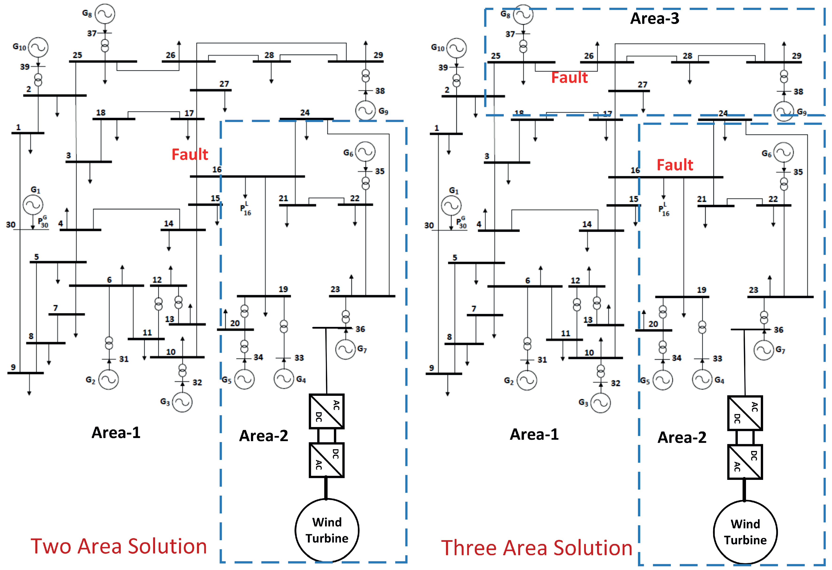
Figure 1. The sectionalized grid model. By disconnecting the transmission lines multiple areas can be created.
Energies 13 03494 g001
Figure 2. Top figure: Rotor angle instability observed once the critical fault is cleared. Bottom figure: Rotor speed fluctuation observed right after the three phase fault.
Energies 13 03494 g002
Figure 3. Top figure: High fluctuation in rotor angle due to the critical fault. Mid figure: K-means cluster of two groups of generators. Bottom figure: K-means cluster of three groups of generators.
Energies 13 03494 g003
Figure 4. Workflow of the proposed method. This method is applied in a distributed architecture on each of the synchronous generators.
Energies 13 03494 g004
Figure 5. The governor and exciter control with an added functional block for the proposed secondary control.
Energies 13 03494 g005
Figure 6. Top three figures are showing the three different time-lines. The bottom figure represents time-line-2&3 in the case when the proposed algorithm successfully restores the system.
Energies 13 03494 g006aEnergies 13 03494 g006b
Figure 7. Top figure: Time series data of Generator-7 under different scenarios. Bottom figure: Normalized 1st principle component of ‘timeline-1’under three different contingencies.
Energies 13 03494 g007
Figure 8. Variation Observed in the normalized 1st-PCs obtained from different events in generator-1 data. Each PC shown here, represents the near-end stage of one power system event
Energies 13 03494 g008
Figure 9. Peak prominence and width inside a predefined data window of the Terminal voltage of Generator-1.
Energies 13 03494 g009
Figure 10. Available frequencies. The sum of all the available frequencies is presented as the frequency factor.
Energies 13 03494 g010
Figure 11. Sensitivity P M / V f b u s Curve.
Energies 13 03494 g011
Figure 12. A set of example decisions: Observed from individual generator under different scenarios and an instance of statistical voting observed from all the generators under one scenario.
Energies 13 03494 g012
Figure 13. An instance of the proposed classification process in Generator-4. (a) The tree that selects active power reference using features (b) The tree that carries out priority voting.
Energies 13 03494 g013
Figure 14. Three cases of grid restoration. (a) No segmentation solution, (b) Two-area solution, (c) Three-area solution.
Energies 13 03494 g014
Figure 15. Prediction accuracy with the test data (two-area solution). The comparison shows a clear improvement with the proposed feature-base method.
Energies 13 03494 g015
Figure 16. Ramifications of the ‘Classification Error’. Top figure: Misclassification in active power referencing. Bottom figure: Misclassification in load-shedding; (a) Instability observed after grid restoration, (b) Instability observed after islanding, (c) Instability observed after the load has been restored.
Energies 13 03494 g016
Table 1. List of stochastic contingencies.
DecisionsWind Speed (m/s)Variable Demand (MW)Contingencies
110546Loss of Genearator-4. No segmentation is required
212609Loss of Genearator-9. No segmentation is required
38405Three phase fault at Bus-16. Two area segmentation
41235Three phase fault at Bus-19. Two area segmentation
58.2662Three phase fault at Bus-16 and Bus-25. Three area segmentation
............
............
n11.2408Three phase fault at Bus-25 and loss of Generator-4. Three area segmentation
Table 2. Distributed decision table for generator-4. Contingencies leading to a two area solution.
DecisionsWind Speed (m/s)Variable Demand (MW)Snsvt (Sensitivity)Prmn (Prominence)FF (Frequency Factor)
112350.138434.1197.4
261450.13330.65934.48
384050.16360.05667.5878
............
............
n117900.14240.59325.2
Table 3. Distributed decision table for generator-4. Contingencies leading to a three area solution.
DecisionsWind Speed (m/s)Variable Demand (MW)Snsvt (Fault-1)Snsvt (Fault-2)Prmn (Prominence)FF (Frequency Factor)
18.26620.87701.01950.437413.7012
2103720.93490.99100.7647178.1212
..............
..............
n11.24080.85150.27790.709932.4
Table 4. Distributed decision table for generator-4. Contingencies are not followed by multiple area segmentation.
DecisionsWind Speed (m/s)Variable Demand (MW)Snsvt (Sensitivity)Prmn (Prominence)FF (Frequency Factor)
19.99652520.21920.000846.7454
2105460.21190.254146.8115
............
............
n126090.15470.12919.56
Table 5. Comparison in accuracies for Timeline-1 in Percent %.
GeneratorProposed MethodEnsemble of Clusters and Decision TreeANNPCA and Decision Tree
496.289.4<4083.71
596.496.4<4082.02
694.6494.56<4084.2
795.0893.33<4065.72
894.3290.17<4067.23
995.4892.8<4066.49
1093.891.1<4089.7