Article

Improved Appliance Classification in Non-Intrusive Load Monitoring Using Weighted Recurrence Graph and Convolutional Neural Networks

1
Ireland’s National Centre for Applied Data Analytics (CeADER), University College Dublin, Dublin 4, Ireland
2
ITI, LARSyS, Técnico Lisboa, 1049-001 Lisboa, Portugal
*
Author to whom correspondence should be addressed.
Energies 2020, 13(13), 3374; https://doi.org/10.3390/en13133374
Submission received: 13 May 2020 / Revised: 15 June 2020 / Accepted: 19 June 2020 / Published: 1 July 2020

Abstract

:
Appliance recognition is one of the vital sub-tasks of NILM in which a machine learning classier is used to detect and recognize active appliances from power measurements. The performance of the appliance classifier highly depends on the signal features used to characterize the loads. Recently, different appliance features derived from the voltage–current (V–I) waveforms have been extensively used to describe appliances. However, the performance of V–I-based approaches is still unsatisfactory as it is still not distinctive enough to recognize devices that fall into the same category. Instead, we propose an appliance recognition method utilizing the recurrence graph (RG) technique and convolutional neural networks (CNNs). We introduce the weighted recurrent graph (WRG) generation that, given one-cycle current and voltage, produces an image-like representation with more values than the binary output created by RG. Experimental results on three different sub-metered datasets show that the proposed WRG-based image representation provides superior feature representation and, therefore, improves classification performance compared to V–I-based features.

1. Introduction

The introduction of smart meters as part of smart grids will produce quantities of data energy consumption data at very fast rates. Analysis of these data streams offers a lot of exciting opportunities for understanding energy consumption patterns. Understanding the consumption pattern of individual loads at consumer premises plays an essential role in the design of customized energy efficiency and energy demand management strategies [1]. It is also useful for improving energy consumption awareness to households, which is likely to stimulate energy-saving behavior and engage energy users towards sustainable energy consumption [2,3]. Non-intrusive Load Monitoring (NILM), also known as energy disaggregation, is a useful technique for analyzing energy consumption data, monitored from a single-point source such as a smart meter. This is because the method can be easily integrated with buildings. The operation of NILM relies on signal processing and machine learning techniques to extract individual load profile from aggregate signal [4,5]. Considerable research attention has been lately devoted to deep neural networks (DNN) to solve energy disaggregation problems [6,7,8,9,10,11,12]. The presented approaches can be classified into event-based and non-event based methods [13]. The former approaches seek to disaggregate appliances through detecting and classifying their transitions in the aggregated signal [9,10,12,14]. In contrast, the non-event-based methods attempt to match each sample of the aggregated signal to the consumption of one or more appliances [6,7,8,11]. This paper falls under the event-based approach.
A typical event-based NILM system often involves four main steps, data acquisition, event detection, appliance classification, and energy estimation [15]. Appliance classification, also known as load identification, is an essential sub-task for identifying the type and status of an unknown load from appliance features extracted from the aggregate power signal. [10]. Therefore, it is imperative to build robust classification models for effective NILM [14]. On the other hand, the performance of classification models highly depends on the appliance features used to characterize appliances [16]. Henceforth, there is a need to develop appliance features that best characterize appliances and improve classification performance.
Appliance features are electrical characteristics of the appliance collected after the state-transition of the device has been detected. In practice, appliance features are obtained from high-frequency or low-frequency measurements, depending on what electrical characteristics are required for NILM. Compared to low-sampling measurements, high-sampling data offer the possibility to consider fine-grained features from steady-state and transient behavior. Typical appliance features at the high frequency used in the literature include transient and harmonics, harmonic contents of current or power waveforms, spectral envelope, wavelet-based feature, and voltage–current (V–I) trajectories [17]. Several recent studies have explored the use of V–I trajectory to characterize appliances [9,10,12,14,16,18,19,20,21]. A V–I-trajectory is obtained by plotting one-cycle steady-state voltage and current. The use of V–I-based features for appliance classification was first introduced in [18], where wave-shape features were hand-engineered the from a V-I trajectory (e.g., number of self-interceptions), and used as input to supervised machine learning classifiers. A review and performance evaluation of seven load wave-shape is presented in [22]. The wave-based features were found to have a direct correspondence to operating characteristics of appliances, and several other features such as peak of middle segment and asymmetry were later developed and evaluated in [20].
However, this approach compresses the information in the V–I-trajectory into a limited amount of hand-engineering feature space. Other studies have shown that transforming the V–I trajectory into a visual representation is computationally efficient and improves classification performance [16,21] by allowing that advanced machine learning algorithms extract features that would be otherwise unobserved.
In [16,21], the V–I trajectory is transformed into a 2D image representation by meshing the V–I trajectory where each cell of the mesh is assigned a binary value and denotes whether or not the trajectory traverses it. The work by [16] extracted several other features, such as the number of continuums of occupied cells, the binary value of the left horizontal cell, and a central cell, from the 2D V–I images. In [9,10,21], the V–I image is used as a direct input to a machine learning classifier such as random forest and convolutional neural networks (CNNs). A hardware implementation of the appliance recognition system based on V–I curves and convolutional neural network (CNN) classier is proposed in [14]. Recently, it has been demonstrated that the visual representation of V–I trajectory can be used effectively with transfer learning [12].
Even though V–I image representation has been successfully used for appliance classification in NILM, its performance is still unsatisfactory since this representation is still not distinctive enough to recognize appliances that fall into the same category. This is because the V–Is have the same shape independently of the current magnitude, which substantially reduces their discerning ability.
Motivated by the quest to create strong feature representation and improve classification performance, in this study, we propose new feature representation for appliance classification which relies on the recurrence graph (RG), also known as the recurrence plot. The RG analyses signal dynamics in phase–space to reveal the repeating and non-linear patterns [23] and has been used extensively for feature representation in time-series classification problems [23,24,25]. Unlike the V–I image, the RG feature representation uses a distance-similarity matrix to represent and visualize structural patterns in the signal. As a consequence, RG feature representation also depends on the magnitude of the current and voltage signals.
RG’s use for the characterization of appliances features was introduced in [26], and later Rajabi and Estebsari [27] applied RG for estimating power consumption of individual loads. However, similar to other RG methods for time-series classification, the proposed RG uses a compressed distance function that represents all recurrences in the form of a binary matrix. Binarizing the recurrence plot through thresholding is likely to cause information loss and degrade classification performance. To avoid information loss by binarization, we propose the generation of RG that gives a few more values instead of binary output. To classify the generated RG, we follow the approach used in [10] and apply CNN for this task. Experimental evaluation in the three sub-metered datasets shows that the proposed WRG feature representation offers superior performance when compared to the V–I-based image feature. The source code used in our experiments can be found on a GitHub repository (https://github.com/sambaiga/WRG-NILM).
The main contributions of this paper are listed as follows:
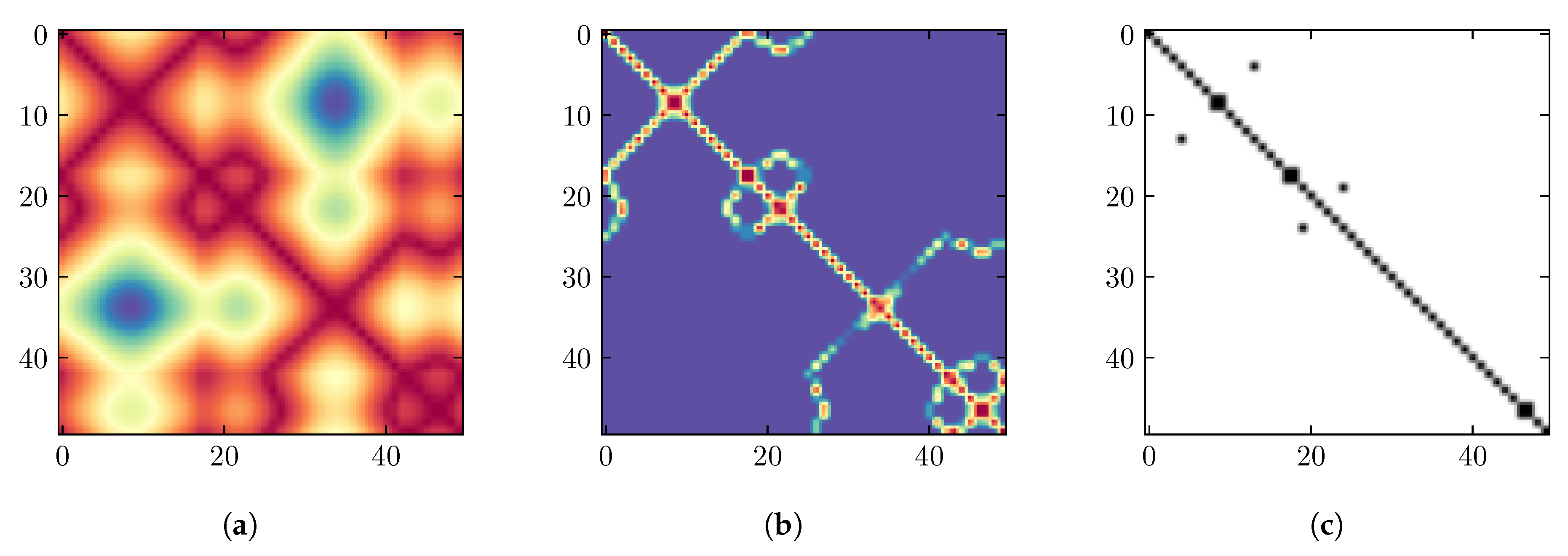
  • We present a recurrence graph feature representation that gives a few more values (WRG) instead of the binary output, which improves the robustness of appliance recognition. The WRG representation for activation current and voltage not only enhances appliance classification performance but also guarantees the appliance feature’s uniqueness, which is highly desirable for generalization purposes.
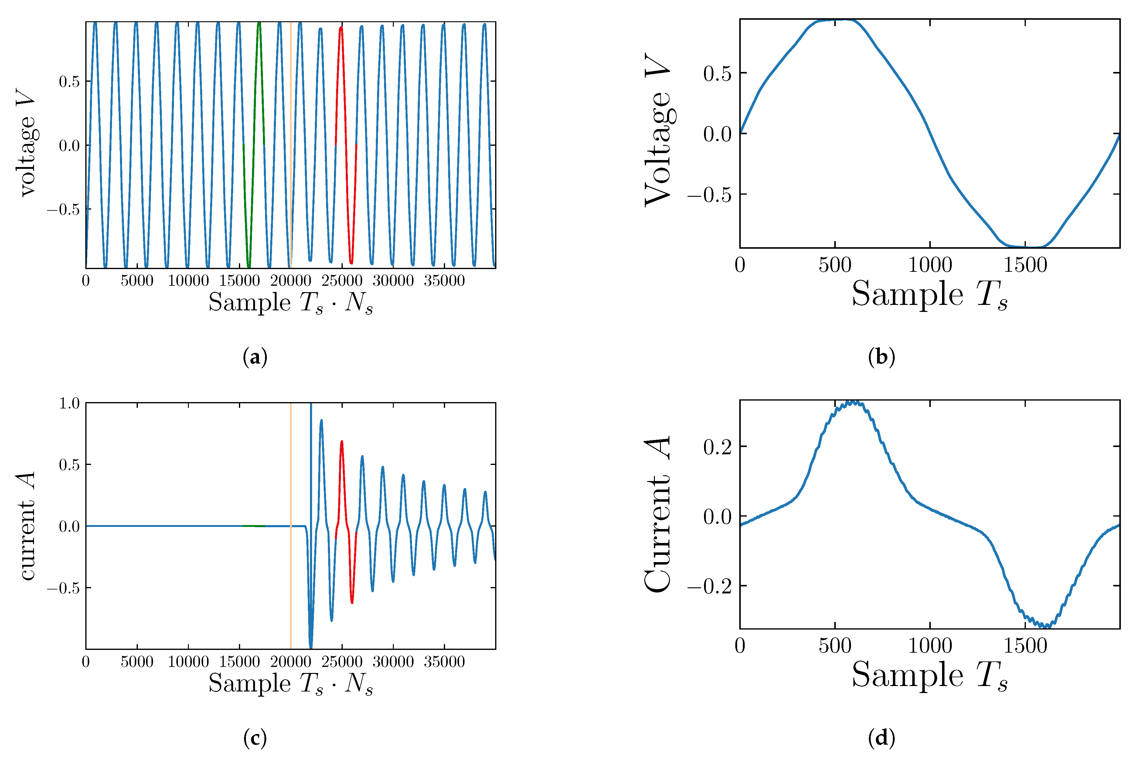
  • We present a novel pre-processing procedure for extracting steady-state cycle activation current from current and voltage measurements. The pre-processing method ensures that the selected activation current is not a transient signal.
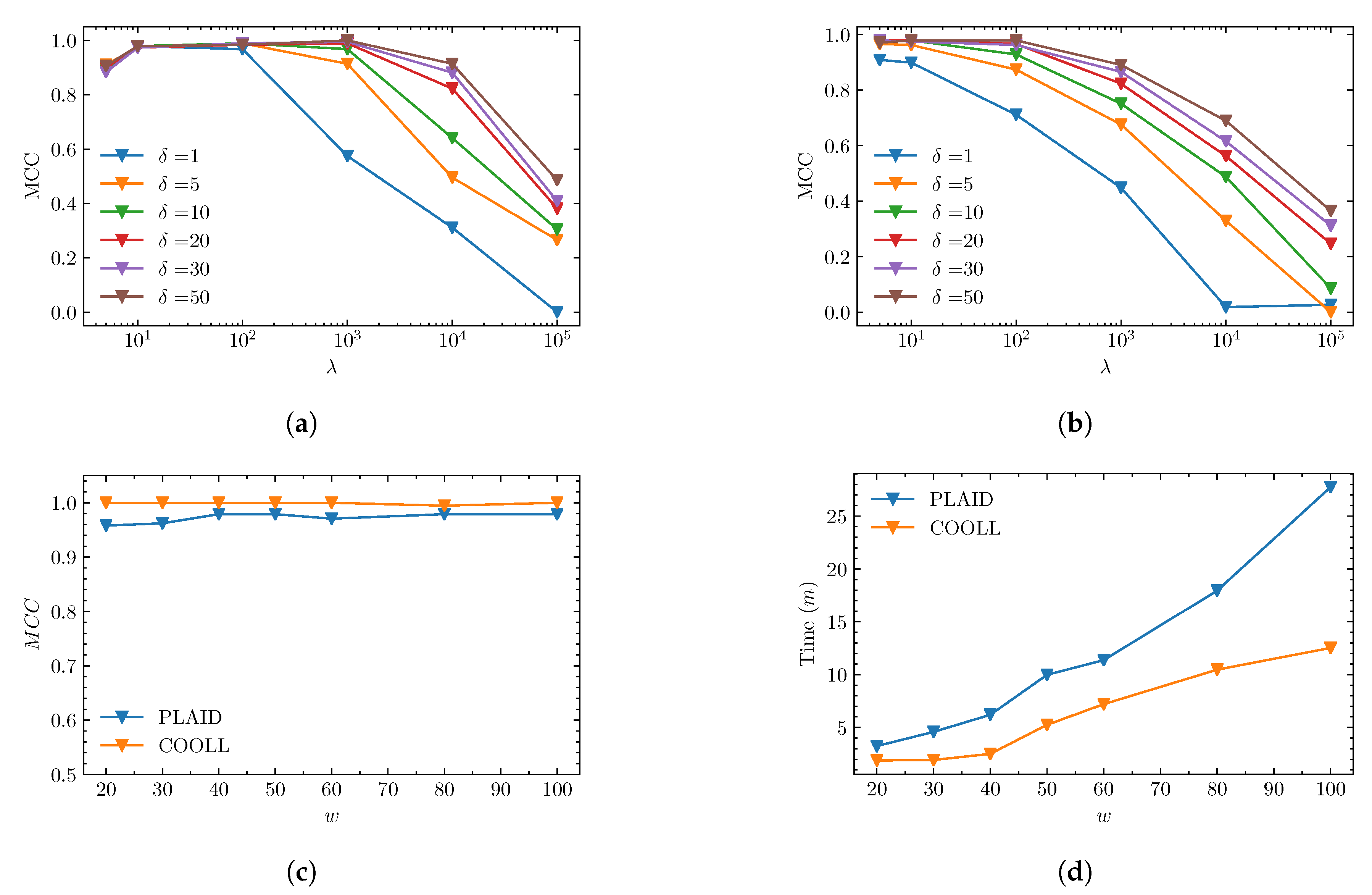
  • We conduct evaluations on three sub-metered public datasets and comparing with the V–I image, which is its most direct competitor. We also conduct an empirical investigation on how different parameters of the proposed WRG influence classification performance.
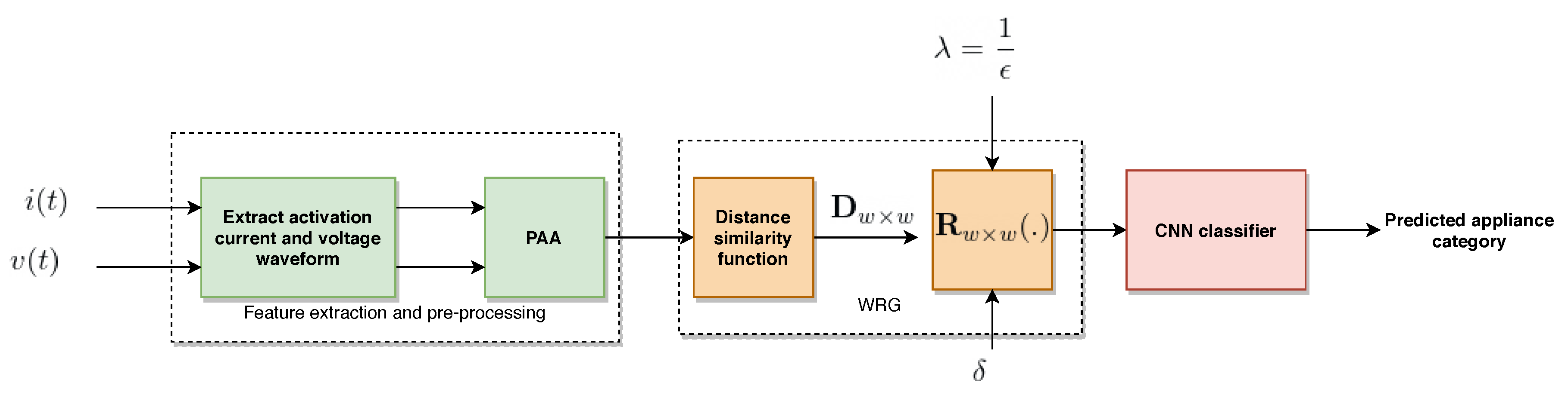
2. Proposed Methods

Recognizing the appliance from the aggregate power signal is a vital sub-task of NILM. The goal of appliance classifier in NILM is to identify active appliances k { i = 1 , 2 , M } from aggregate signal x t where M indicates the number of appliances. This is a multi-class classification problem. The aggregate signal x t at any time t is assumed to be
x t = k M y t ( k ) · s t ( k ) + σ t
where y t ( k ) is the contribution of appliance k, s t ( k ) { 0 , 1 } is its state and σ t represents both any contribution from appliances not accounted for and measurement noise. The proposed approach is summarized Figure 1 and consist of the following main building blocks; Feature extraction and pre-processing, WRG generation and the CNN classifier.

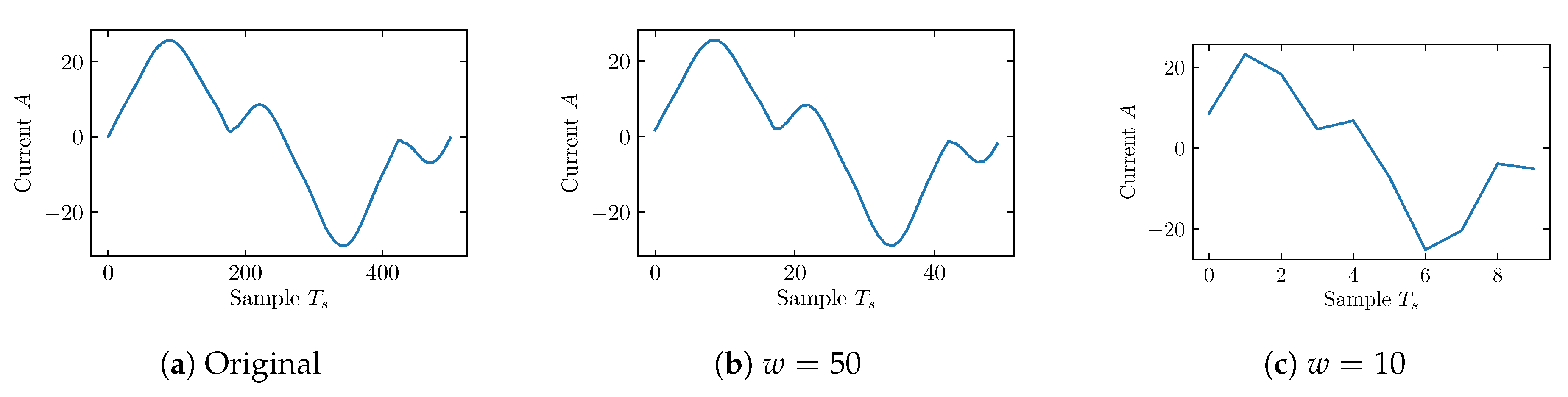
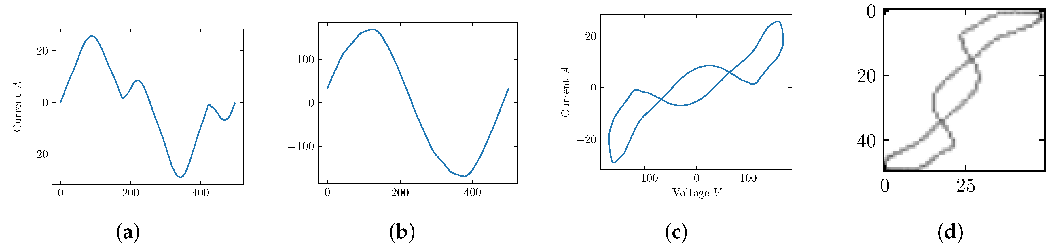
2.1. Feature Extraction and Pre-Processing

Appliance features used for appliance recognition can be categorized into snapshot-form or delta-form features [22]. Snapshot form refers to the appliance feature extracted from aggregate power measurements as the results of more than one appliance being activated. Delta-form, on the other hand, expresses load characteristics in brief windows of time containing the only single event. In this work, we consider delta-form appliance features and define an activation signal as a one-cycle steady-state signal extracted from current or voltage waveform in a brief time after state transition.
To obtain an activation signal from monitored power signals; we measure N s = 20 cycles of v and i before and after state-transitions of appliance has been detected as shown in Figure 2a,c. The N s cycles correspond to steady-state behavior and is equivalent to T s × N s samples where T s = f s f , f s is sampling frequency and f is mains frequency. Since in this work, we only consider sub-metered data, the activation current i and voltage v from current-voltage signals is obtained as follows: i = i ( a ) and v = v ( a ) if the event is caused by activation of appliance and i = i b and v = v b if the event is caused by de-activation of appliance as illustrated in Figure 2b,d.
To remove noise and ensure that the obtained activation signal is a complete cycle with size T s , we propose a pre-processing procedure summarized in 1. This is an empirical method and is based on the engineering knowledge that steady-state activation current should have at least two zero-crossings.
Algorithm 1: Feature pre-processing
Result: i j , v j
Data: i 1 N , v 1 N
Get voltage zero crossings: zc v ;
Energies 13 03374 i001
Once activation-waveforms have been extracted, the piece-wise aggregate approximation (PAA) is used to reduce the dimensional of the signal from T s to a predefined size w with minimal information loss. The PAA algorithm reduces the dimensionality of i and v from T s to embedding size w before generating the D w × w distance matrix. It works by dividing the data into n segments of equal size, then the approximation is a vector of the median values of the data readings per segment. The embedding size w is the hyper-parameter that needs to be selected in advance. Empirically, it was found that the choice of w does not significantly influence the classification performance. However, large values of w impact the learning speed, and small values of w will most likely lead to larger information loss, as depicted in Figure 3. Note that for Figure 3b the embedding size of w = 50 does not change the shape of the input signal, whereas in Figure 3c an embedding size of w = 10 deforms the input shape.

2.2. Weighted Recurrence Plot (WRG)

The RG feature representation uses a distance similarity matrix D w × w to represent and visualize structural patterns in the signal. The distance similarity matrix provides a relationship metric between each element in the time-series signal [28]. It has been recommended as a pre-processing step for many of the machine learning approaches such as K-means clustering and K-nearest neighbor algorithms. Consider T s points of activation signal x = { x 1 , x 2 x T s } . The distance similarity between x k and x j is given as d k , j = | | x k x j | | 2 where | | . | | denotes the Euclidean norm. The distance similarity matrix D w × w = [ d k , j ] is the similarity matrix such that:
D w × w = d 1 , 1 d 1 , j d k , 1 d k , j
For a classification problem, the compressed distance similarity matrix that represents all recurrences in the form of a binary matrix R G w × w = [ r k , j ] is usually used. The r k , j function is defined as follows:
r k , j = 1 if d k , j ϵ 0 otherwise
where ϵ ( 0 , 1 ] is the recurrence threshold. Equation (3) implies that, a dot will be drawn on a w × w grid if two values within a signal x = { x 1 , x 2 , x w } are closer than ϵ .
This can be interpreted as unweighed graph G with vertex set N and edge E where R G w × w = [ r k , j ] is the adjacency matrix that depicts the graph between the data points. It should be noted that the structural representation of RG provides the similarity between two adjacent points in time series which is necessary for classification [29]. However, binarizing the distance matrix D w × w through thresholding can lead to information loss and therefore degrade classification performance. Thus in this work, we propose the generation of W R G w × w that goes beyond the traditional binary output. More precisely, we introduce the parameter δ 1 that enforce r k , j to have values between 0 and δ such that:
r k , j = δ if τ > δ τ otherwise
where τ = d k , j ϵ . . is the floor function such x = n x ( n + 1 ) , 0 n δ , ϵ 0 .
For computational stability, we apply the parametrization on the value of ϵ such that λ = 1 ϵ . The matrix W R G w × w can be interpreted as a weighted graph G = ( V , E ) where each value represents the edge weights. Since d k , j > 0 Equation (4) reduces to RG for δ 1 . The recurrence threshold ϵ and δ are the hyper-parameters that need to be optimized. Figure 4 illustrates the process of generating the WRG and RG from distance similarity matrix D. We see that the RG image representation in Figure 4c has more limited information compared to the WRG image representation in Figure 4b.

2.3. Classifier and Training Procedure

Once the appliance features are extracted, a generic machine learning classifier can be used to learn the pattern from labeled data. We consider a convolution neural network (CNN) for this task. CNNs are specific kinds of neural networks for processing visual data. They leverage local connectivity and equivariant representations that make CNN useful for computer vision tasks. Each hidden unit of a CNN layer is connected only to the subregion of the input image. This allows CNNs to exploit spatially local correlation between neurons of adjacent layers while reducing the number of parameters. Thus, at each CNN layer, the classifier learns several small filters (feature maps). These feature maps are then applied to the entire layer, allowing features to be detected regardless of their position in the image.
The CNN network applied in this work consists of three-stages 2D CNN layers each with 16 , 32 and 64 feature maps, 3 × 3 filter, 2 × 1 stride and padding of 1. Each CNN layer is followed by batch normalization (BN) block and Leaky relu activation functions. The final layer consists of one flatten layer and two Fully connected layers (FC) layers. The FC layers have a hidden size of 1024 and K, respectively, where the number of appliances available determines the number of classes (K). The final predicted class is obtained by applying softmax activation function. To learn the model parameters, a standard back propagation is used to optimize the cross-entropy objective function defined in Equation (5):
L θ ( y , p ) = i = 1 M y i · log p i
Specifically the mini-batch Stochastic Gradient Descent (SDG) with a momentum of 0.9 , a learning rate of 0.001 , and a batch size of 16 is used to train the model for 100 iterations. To avoid over-fitting, early stopping with patience is used where the traing is terminated once the validation performance does not change after 20 iterations.

3. Experimental Design

3.1. Datasets

The proposed method is tested on the three publicly accessible datasets; Plug Load Appliance Identification Dataset (PLAID v1) [30], Worldwide Household and Industry Transient Energy Data Set (WHITED v1.1) [31], and Controlled On/Off Loads Library (COOLL) datasets [32]. The PLAID v1 contains 1074 instances of current and voltage measurements sampled at 30 kHz from 11 different appliance types in Pittsburgh, Pennsylvania, USA. Each appliance type is represented by various samples of varying make/models. The WHITED consists of sub-metered current and voltage measurements recorded in households and small industry settings at 44.1 KHz sampling frequency. In this work, we use the WHITED v1.1 that comprises 11259 instances for 110 various appliances, which can be grouped into 47 different types (classes).
The COOLL dataset, on the other hand, consists of d 840 current and voltage measurements for 42 controllable appliances sampled at a 100 kHz sampling frequency. Unlike PLAID and WHITED datasets, the COOLL dataset provides twenty turn-on transient signals corresponding to a different turn-on instant (with a controlled delay to the zero-crossing of the mains voltage) for each appliance. The appliances are of 12 different types with a certain number of examples each [32].

3.2. Evaluation Metrics

Several performance metrics have been proposed in the NILM literature [13]. This work uses macro averaged F 1 score, zero-loss score (ZL) and Matthews correlation coefficient (MCC), as these are known for being less sensitive to class imbalance [33]. We also use the confusion matrix which shows the correct predictions (the diagonal) and provide a clear view on which appliances are confused with each other.
The F 1 (%) score is defined as F m a c r o = 100 · 1 M i = 1 M F 1 ( i ) where M is the number of appliances and F 1 is the harmonic mean of precision and recall.
The zero-loss give the number of miss-classifications with the best performance being 0 and is defined as Z L = i = 1 M I ( y i y ^ i ) The Matthews correlation coefficient, MCC, provides a balanced performance measure of the quality of classification algorithm. It takes into account true and false positives and negatives. Given confusion matrix C for M different classes, the MCC can be defined as
M C C = c × s i M p i × t i ( s 2 i M p i 2 ) × ( s 2 i M t i 2 )
where t i = k M C k i , p i = k M C i k , c = k M C k k , and s = i M j M C i j . The maximum MCC score is +1 and the minimum value can be between −1 and 0. A score of +1 represents a perfect prediction.

3.3. Experimental Description

We are interested in answering the following two research questions: (1) how to pick a suitable set of WRG hyper-parameters? And, (2) how do the graph features extracted by WRG compare against V–I based approach concerning classification performance? We investigate the first objective by altering the WRG hyper-parameters w, δ , and λ = 1 / ϵ on the PLAID, and COOLL sub-metered datasets. We first investigate how do the λ and δ parameters influence performance measure when the embedding size is set to 50 ( w = 50 ). We then analyze the impact of the embedding size w on classification performance for given values of λ and δ . We further compare the general performance between the binary RP and WRG.
In the second experiment, we establish a baseline in which the V–I binary image is used as the appliance feature. The baseline is then compared with the WRG feature representation. The V–I image of size w × w , is obtained by first resizing the activation current i and voltage v into corresponding scale d i and d v respectively where: d c = max ( | min ( i ) | , max ( i ) ) and d v = max ( | min ( v ) | , max ( v ) ) and transformed into w × w scale. The scaled current and voltage are then converted into w × w image by meshing the V–I trajectory and assigned a binary value that denotes whether it is traversed by trajectory as described in De Baets et al. [10]. Figure 5 illustrate the generation of V–I image from microwave activation current and voltage in the PLAID dataset.
The objective of this experiment is to compare the generalization performance of the proposed approach with that of VI across buildings. To achieve this, we employ leave-one-house-out cross-validation as presented in [21]. A classifier is trained on a dataset in N b 1 houses and then tested using the unseen house in the same dataset. However, unlike PLAID, the WHITED and COOLL datasets do not have household annotations. Therefore, we adopt the method used in [10], which consists of assigning appliances randomly to artificial homes. The total number of houses is set to 9 for the WHITED dataset and 8 for the COOLL dataset, corresponding to the minimum number of appliance types in each dataset.
The parameters used in this experiment are presented in Table 1.

4. Results and Discussion

This section presents and discusses the results obtained with respect to the two research objectives of this paper.

4.1. Objective 1: WRG Analysis

In the first objective, we investigate how do WRG parameters w, λ and δ influence performance measure. Figure 6a,b shows the relationship between λ and M C C score for different value δ on COOLL and PLAID datasets.
From Figure 6b, we observe that in PLAID a maximum score of 0.981 M C C is reached, when λ = 10 1 and δ = 20 . It can be also observed from Figure 6a, that in COOLL, a maximum score of 1.0 M C C is reached for λ = 10 3 and δ = 50 . We further see that the binary RG ( when δ = 1 ) achieves a maximum score of 0.97 M C C (when λ = 10 ) in COOLL, and 0.90 M C C (when λ = 5 ) in PLAID. However, the performance drops rapidly as λ increases and eventually become zero in PLAID. We also observe that the influence of δ on performance score depends on the selected value of λ . For larger values of λ , the performance increases as δ increases. In contrast, for small values of λ , δ does not significantly impact the performance score.
We also investigate the influence of embedding size w in the classification performance as depicted in Figure 6c. We see that the higher value of w does not significantly improve classification performance. This result is in line with the one obtained in [9] for the V–I image, which concluded that, once a particular resolution is obtained, adding information by increasing the embedding size does not improve performance. Nevertheless, a significantly high value of w impacts the learning speed as shown in Figure 6d. Also as discussed in the feature extraction and pre-processing subsection, a low value of w might lead to information loss, thereby degrading the performance score. Finally, we compare the general performance between the binary RG and WRG, as tabulated in Table 2. We see that compared to binary RG, the proposed WRG improves classification performance from 98.96 % to 99.86 % F 1 score for the COOLL dataset and 88.18 % to 94.35 % F 1 score for the PLAID dataset.

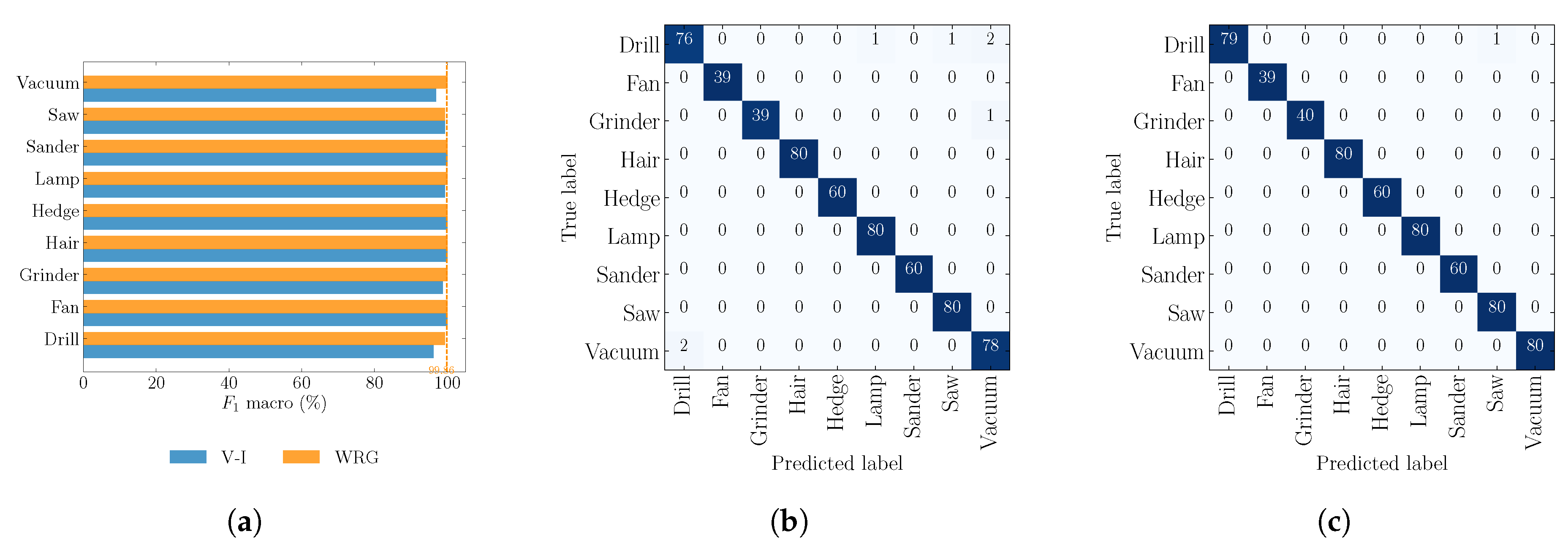
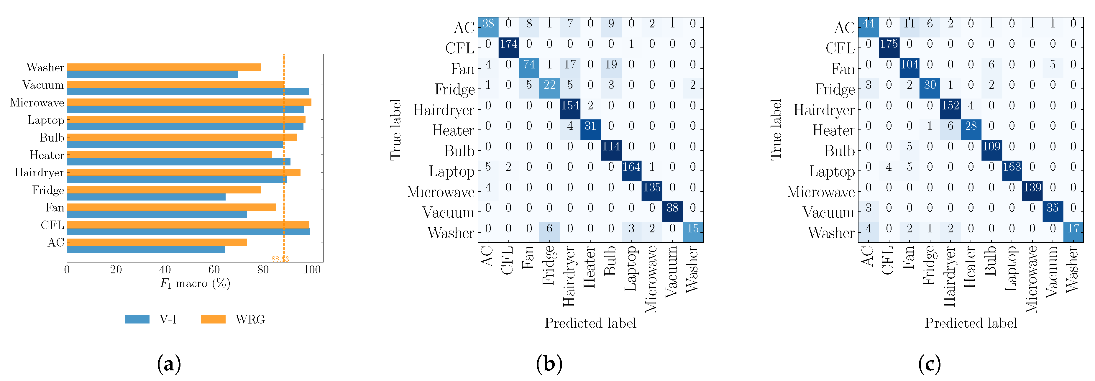
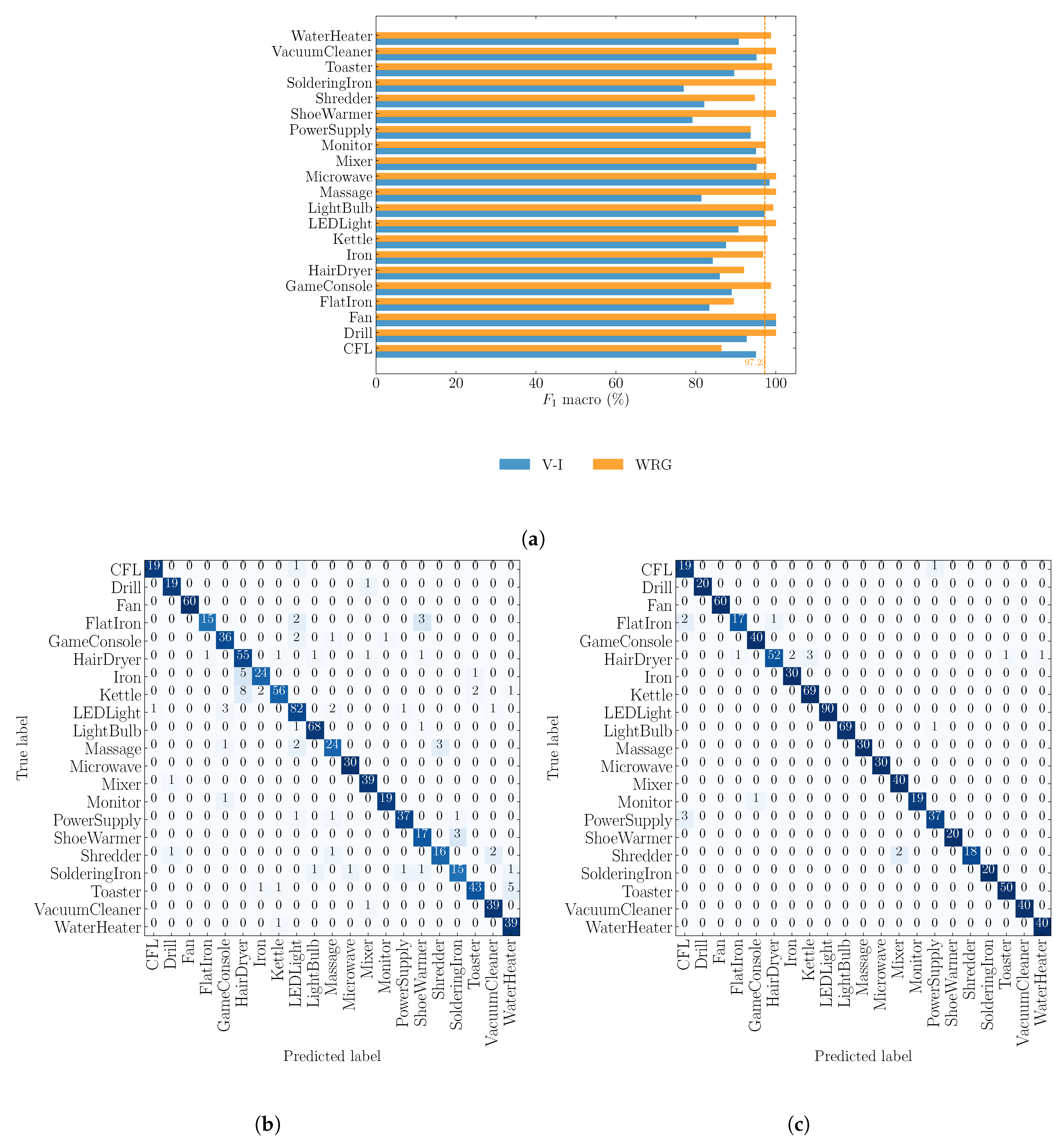
4.2. Objective 2: Comparison against V–I Image Method

In this experiment, we compare the generalization performance of the WRG and V–I image representation across multiple buildings. We first present and discuss the overall performance of the three sub-metered datasets, as listed in Table 3. From the results presented in Table 3, we see that WRG out-performs the V–I image in all three datasets with 0.92 % , 8.5 % , and 4.5 % percentage points increase in F 1 macro for COOLL, WHITED and PLAID dataset respectively.
For benchmarking purposes, the results presented in this paper are compared with the ones presented in [10] for WHITED and PLAID datasets. We see an increase in F 1 macro score from 77 % to 88.53 % on PLAID and from 75.46 % to 97.23 on the WHITED dataset. Ultimately, these results demonstrate the effectiveness of the WRG feature in characterizing appliances across multiple buildings. We also see the improved performance on the presented V–I based CNN. Yet, the increase in F 1 macro score is attributed to the improved pre-prepossessing procedure and developed CNN model architecture.
We also present and discuss the per-appliance performance on the three datasets. Figure 7 shows the F 1 macro (%) per appliance for the COOLL dataset. It can be observed in Figure 7a that except for two appliances (Saw and Hedge), the F 1 macro (%) is above 99.0 % for WRG. Examining the confusion matrix for the V–I image in Figure 7b, we see that the V–I makes four confusions between Vacuum and Drill (all having rotating components), one confusion between Vaccum and Grinder, Drill and Lamp and between Drill and Lamp. The use of WRG reduces these confusions to only one confusion, between Saw and Drilling machine (all having rotating components) as depicted in Figure 7c.
Figure 8a presents the per appliance F 1 macro (%) for the PLAID dataset. From Figure 8a, we see that with exception to Washer, Heater, Fridge, AC, and Fan, the WRG reaches at least 88 % F 1 macro score for all other appliances. Observing the confusion matrix for WRG in Figure 8c and V–I image in Figure 8c, we see WRG reduces most of the confusions. More precisely, between Fan and Hairdryer (from 19 to 0), Fan and Bulb (from 19 to 6), Fridge and Washer (from 6 to 1) and between AC and other appliances (from 25 to 23). However, despite the increase performance, the WRG makes four confusions between Washer and AC, and five confusions between Fan and Vacuum (both having motor).
Finally, Figure 9a presents results for the WHITED dataset. We see that for the WRG, most appliances achieve 97.0 F 1 macro and above. The exceptions are the PowerSupply, Shredder, Hairdryer, Flat Iron, and CFL. From the confusion matrix Figure 9b, we observe that for V–I image representation, the HairDryer is confused with the Iron (9) and kettle (6) (both having heating elements); however, the WRG reduces these confusions to 5 as shown in Figure 9c.

5. Conclusions and Future Work Directions

In this paper, we presented a WRG-based feature representation for appliance classification in NILM. Specifically, we propose a variation of the RG plot that goes beyond the traditional binary outputs. By following this non-binary approach, the proposed method ensures that more information is preserved in the RG, thus improving its discriminant power.
Extensive evaluations using CNNs for classification, and three public sub-metered datasets show that the proposed WRG feature consistently improves the appliance classification performance compared to the commonly used V–I image representation.
We further assessed how WRG’s hyper-parameters influence classification performance. We found that the hyper-parameters are dataset dependent, which raises another fundamental research question: how these parameters can be selected and if they are related to data characteristics like sampling frequency. In future work, we will investigate appropriate methods for choosing these parameters. Precisely, we will investigate whether the WRG hyper-parameters could be treated as learn-able parameters like standard neural network weights.
Finally, even though the proposed approach was evaluated against three public datasets, it is essential to remark that these are all sub-metered. Therefore, future work should also assess the WRG on aggregated datasets. Furthermore, when considering aggregated data, it is also essential to determine the impact of the event detection algorithms (e.g., [34,35]) in the extraction of the current activation waveforms. Moreover, relying on aggregate datasets also presents the opportunity of exploring the applicability of the proposed WRG feature for multilabel appliance classification.

Author Contributions

Conceptualization, A.F.; Data curation, A.F.; Formal analysis, A.F. and L.P.; Methodology, A.F. and L.P.; Resources, A.F.; Software, A.F.; Supervision, L.P.; Validation, L.P.; Writing—original draft, A.F.; Writing—review & editing, A.F. and L.P. All authors have read and agreed to the published version of the manuscript.

Funding

Lucas Pereira has received funding from the Portuguese Foundation for Science and Technology (FCT) under grants CEECIND/01179/2017 and UIDB/50009/2020.

Conflicts of Interest

The authors declare no conflict of interest.

References

  1. Cominola, A.; Giuliani, M.; Piga, D.; Castelletti, A.; Rizzoli, A. A Hybrid Signature-based Iterative Disaggregation algorithm for Non-Intrusive Load Monitoring. Appl. Energy 2017, 185, 331–344. [Google Scholar] [CrossRef]
  2. Batra, N.; Singh, A.; Whitehouse, K. If You Measure It, Can You Improve It? Exploring The Value of Energy Disaggregation. In Proceedings of the 2nd ACM International Conference on Embedded Systems for Energy-Efficient Built Environments (BuildSys ’15), Seoul, Korea, 4–5 November 2015; pp. 191–200. [Google Scholar] [CrossRef]
  3. Huss, A. Hybrid Model Approach to Appliance Load Disaggregation. Ph.D. Thesis, KTH Royal Institute of Technology, Stockholm, Sweden, 2015. [Google Scholar]
  4. Kelly, J.; Knottenbelt, W. The UK-DALE dataset, domestic appliance-level electricity demand and whole-house demand from five UK homes. Sci. Data 2015, 2, 150007. [Google Scholar] [CrossRef] [PubMed] [Green Version]
  5. Makonin, S.; Popowich, F.; Bajić, I.V.; Gill, B.; Bartram, L. Exploiting HMM Sparsity to Perform Online Real-Time Nonintrusive Load Monitoring. IEEE Trans. Smart Grid 2016, 7, 2575–25857. [Google Scholar] [CrossRef]
  6. Kelly, J.; Knottenbelt, W. Neural nilm: Deep neural networks applied to energy disaggregation. In Proceedings of the 2nd ACM International Conference on Embedded Systems for Energy-Efficient Built Environments, Seoul, Korea, 4–5 November 2015; pp. 55–64. [Google Scholar]
  7. Zhang, C.; Zhong, M.; Wang, Z.; Goddard, N.; Sutton, C. Sequence-to-point learning with neural networks for non-intrusive load monitoring. In Proceedings of the Thirty-Second AAAI Conference on Artificial Intelligence, New Orleans, LA, USA, 2–7 February 2017. [Google Scholar]
  8. Murray, D.; Stankovic, L.; Stankovic, V.; Lulic, S.; Sladojevic, S. Transferability of Neural Network Approaches for Low-rate Energy Disaggregation. In Proceedings of the 2019 IEEE International Conference on Acoustics, Speech and Signal Processing (ICASSP), Brighton, UK, 12–17 May 2019; pp. 8330–8334. [Google Scholar]
  9. De Baets, L.; Dhaene, T.; Deschrijver, D.; Develder, C.; Berges, M. VI-Based Appliance Classification Using Aggregated Power Consumption Data. In Proceedings of the 2018 IEEE International Conference on Smart Computing (SMARTCOMP), Taormina, Italy, 18–20 June 2018; pp. 179–186. [Google Scholar] [CrossRef] [Green Version]
  10. De Baets, L.; Ruyssinck, J.; Develder, C.; Dhaene, T.; Deschrijver, D. Appliance classification using VI trajectories and convolutional neural networks. Energy Build. 2018, 158, 32–36. [Google Scholar] [CrossRef] [Green Version]
  11. Gomes, E.; Pereira, L. PB-NILM: Pinball Guided Deep Non-Intrusive Load Monitoring. IEEE Access 2020, 8, 48386–48398. [Google Scholar] [CrossRef]
  12. Liu, Y.; Wang, X.; You, W. Non-Intrusive Load Monitoring by Voltage–Current Trajectory Enabled Transfer Learning. IEEE Trans. Smart Grid 2019, 10, 5609–5619. [Google Scholar] [CrossRef]
  13. Pereira, L.; Nunes, N. Performance evaluation in non-intrusive load monitoring: Datasets, metrics, and tools—A review. Wiley Interdiscip. Rev. Data Min. Knowl. Discov. 2018, 8, e1265. [Google Scholar] [CrossRef] [Green Version]
  14. Baptista, D.; Mostafa, S.; Pereira, L.; Sousa, L.; Morgado, D.F. Implementation Strategy of Convolution Neural Networks on Field Programmable Gate Arrays for Appliance Classification Using the Voltage and Current (V–I) Trajectory. Energies 2018, 11, 2460. [Google Scholar] [CrossRef] [Green Version]
  15. Faustine, A.; Mvungi, N.H.; Kaijage, S.; Kisangiri, M. A Survey on Non-Intrusive Load Monitoring Methodies and Techniques for Energy Disaggregation Problem. arXiv 2017, arXiv:1703.00785. [Google Scholar]
  16. Du, L.; He, D.; Harley, R.G.; Habetler, T.G. Electric Load Classification by Binary Voltage–Current Trajectory Mapping. IEEE Trans. Smart Grid 2016, 7, 358–365. [Google Scholar] [CrossRef]
  17. Sadeghianpourhamami, N.; Ruyssinck, J.; Deschrijver, D.; Dhaene, T.; Develder, C. Comprehensive feature selection for appliance classification in NILM. Energy Build. 2017, 151, 98–106. [Google Scholar] [CrossRef] [Green Version]
  18. Lam, H.Y.; Fung, G.S.K.; Lee, W.K. A Novel Method to Construct Taxonomy Electrical Appliances Based on Load Signaturesof. IEEE Trans. Consum. Electron. 2007, 53, 653–660. [Google Scholar] [CrossRef] [Green Version]
  19. Li, L.; Zhao, Y.; Jiang, D.; Zhang, Y.; Wang, F.; Gonzalez, I.; Valentin, E.; Sahli, H. Hybrid Deep Neural Network–Hidden Markov Model (DNN-HMM) Based Speech Emotion Recognition. In Proceedings of the 2013 Humaine Association Conference on Affective Computing and Intelligent Interaction, Geneva, Switzerland, 2–5 September 2013; pp. 312–317. [Google Scholar] [CrossRef]
  20. Wang, A.L.; Chen, B.X.; Wang, C.G.; Hua, D. Non-intrusive load monitoring algorithm based on features of V–I trajectory. Electr. Power Syst. Res. 2018, 157, 134–144. [Google Scholar] [CrossRef]
  21. Gao, J.; Kara, E.C.; Giri, S.; Bergés, M. A feasibility study of automated plug-load identification from high-frequency measurements. In Proceedings of the 2015 IEEE Global Conference on Signal and Information Processing (GlobalSIP), Orlando, FL, USA, 14–16 December 2015; pp. 220–224. [Google Scholar] [CrossRef]
  22. Hassan, T.; Javed, F.; Arshad, N. An Empirical Investigation of V–I Trajectory Based Load Signatures for Non-Intrusive Load Monitoring. IEEE Trans. Smart Grid 2014, 5, 870–878. [Google Scholar] [CrossRef] [Green Version]
  23. Garcia-Ceja, E.; Uddin, M.Z.; Torresen, J. Classification of Recurrence Plots’ Distance Matrices with a Convolutional Neural Network for Activity Recognition. Procedia Comput. Sci. 2018, 130, 157–163. [Google Scholar] [CrossRef]
  24. Hatami, N.; Gavet, Y.; Debayle, J. Classification of Time-Series Images Using Deep Convolutional Neural Networks. arXiv 2017, arXiv:1710.00886. [Google Scholar]
  25. Tsai, Y.; Chen, J.H.; Wang, C. Encoding Candlesticks as Images for Patterns Classification Using Convolutional Neural Networks. arXiv 2019, arXiv:1901.05237. [Google Scholar]
  26. Popescu, F.; Enache, F.; Vizitiu, I.; Ciotîrnae, P. Recurrence Plot Analysis for characterization of appliance load signature. In Proceedings of the 2014 10th International Conference on Communications (COMM), Bucharest, Romania, 29–31 May 2014; pp. 1–4. [Google Scholar] [CrossRef]
  27. Rajabi, R.; Estebsari, A. Deep Learning Based Forecasting of Individual Residential Loads Using Recurrence Plots. In Proceedings of the 2019 IEEE Milan PowerTech, Milan, Italy, 23–27 June 2019; pp. 1–5. [Google Scholar]
  28. Dokmanic, I.; Parhizkar, R.; Ranieri, J.; Vetterli, M. Euclidean Distance Matrices: Essential theory, algorithms, and applications. IEEE Signal Process. Mag. 2015, 32, 12–30. [Google Scholar] [CrossRef] [Green Version]
  29. Tamura, K.; Ichimura, T. MACD-histogram-based recurrence plot: A new representation for time series classification. In Proceedings of the 2017 IEEE 10th International Workshop on Computational Intelligence and Applications (IWCIA), Hiroshima, Japan, 11–12 November 2017; pp. 135–140. [Google Scholar] [CrossRef]
  30. Gao, J.; Giri, S.; Kara, E.C.; Bergés, M. PLAID: A Public Dataset of High-resolution Electrical Appliance Measurements for Load Identification Research: Demo Abstract. In Proceedings of the 1st ACM Conference on Embedded Systems for Energy-Efficient Buildings (BuildSys ’14), Memphis, TN, USA, 3–6 November 2014; ACM: New York, NY, USA, 2014; pp. 198–199. [Google Scholar] [CrossRef]
  31. Kahl, M.; Haq, A.U.; Kriechbaumer, T.; Jacobsen, H.A. WHITED-A Worldwide Household and Industry Transient Energy Data Set. In Proceedings of the 3rd International Workshop on Non-Intrusive Load Monitoring (NILM), Vancouver, BC, Canada, 14–15 May 2016. [Google Scholar]
  32. Picon, T.; Nait Meziane, M.; Ravier, P.; Lamarque, G.; Novello, C.; Le Bunetel, J.C.; Raingeaud, Y. COOLL: Controlled On/Off Loads Library, a Public Dataset of High-Sampled Electrical Signals for Appliance Identification. arXiv 2016, arXiv:1611.05803. [Google Scholar]
  33. Pereira, L.; Nunes, N. A comparison of performance metrics for event classification in Non-Intrusive Load Monitoring. In Proceedings of the 2017 IEEE International Conference on Smart Grid Communications (SmartGridComm), Dresden, Germany, 23–27 October 2017; pp. 159–164. [Google Scholar] [CrossRef]
  34. Pereira, L. Developing and evaluating a probabilistic event detector for non-intrusive load monitoring. In Proceedings of the 2017 Sustainable Internet and ICT for Sustainability (SustainIT), Funchal, Portugal, 6–7 December 2017; IEEE: Funchal, Portugal, 2017; pp. 1–10. [Google Scholar] [CrossRef]
  35. De Baets, L.; Ruyssinck, J.; Develder, C.; Dhaene, T.; Deschrijver, D. On the Bayesian optimization and robustness of event detection methods in NILM. Energy Build. 2017, 145, 57–66. [Google Scholar] [CrossRef] [Green Version]
Figure 1. Block diagram of the proposed approach. It consist of the Feature extraction and pre-processing, WRG generation and the CNN classifier blocks.
Energies 13 03374 g001
Figure 2. Extraction of an activation signal from current and voltage measurements. The green color is the steady-state signal before the event where the steady-state signal after the event is shown in red: (a) Voltage waveforms before and after an event; (b) Activation voltage; (c) Current waveforms before and after events; (d) Activation current.
Energies 13 03374 g002
Figure 3. Illustration of dimension reduction with PAA for different embedding w: (a) The original activation current before dimension reduction; (b) The activation current after PAA with w = 50 . The generated signal resembles the original activation current before PAA; (c) The activation current after PAA with w = 10 . There is a loss of information on the generated signal.
Energies 13 03374 g003
Figure 4. Generation of distance similarity matrix and RGs for a vacuum cleaner activation current in PLAID dataset: (a) Distance similarity matrix D w × w ; (b) WRG matrix W R G w × w ; (c) RG matrix R G w × w .
Energies 13 03374 g004
Figure 5. Generation of V–I image from Microwave activation current and voltage in the PLAID dataset: (a) Activation current; (b) Activation voltage; (c) V–I trajectory; (d) Generated V–I image.
Energies 13 03374 g005
Figure 6. Impact of WRG parameters in the measured performance: (a) Impact of λ for different value of δ on the COOLL dataset; (b) Impact of λ for different value of δ on the PLAID dataset; (c) The relationship between w and M C C score for COOLL and PLAID dataset; (d) The relationship between w and training time on the PLAID and COOLL dataset.
Energies 13 03374 g006
Figure 7. The F 1 macro (%) matrix per appliance and confusion matrix for the COOLL dataset: (a) F 1 macro (%) for V–I and WRG; (b) V–I confusion matrix; (c) WRG confusion matrix.
Energies 13 03374 g007
Figure 8. The F 1 macro (%) matrix per appliance and confusion matrix for the PLAID dataset: (a) F 1 macro (%) for VI and WRG; (b) V–I confusion matrix; (c) WRG confusion matrix; AC = air conditioning, CFL = compact fluorescent lamp, ILB = incandescent light bulb.
Energies 13 03374 g008
Figure 9. The The F 1 macro and confusion matrix for the WHITED dataset: (a) The F 1 macro (%) for the WHITED dataset with V–I and WRG feature representation; (b) WRG confusion matrix.
Energies 13 03374 g009
Table 1. Parameters used in experiment two.
ParameterCOOLLWHITEDPLAID
λ = 1 ϵ 10 3 10 3 10 1
δ 505020
w505050
Table 2. Results comparision between WRG and RG on PLAID and COOLL dataset.
DataMethodMetrics
MCCF1ZL
COOLLRG 0.98 9899 190
WRG 1.00 99.86 0.12
PLAIDRG 0.91 88.18 8.18
WRG 0.97 94.35 2.98
Table 3. Generalisation performance between WRG and VI on PLAID, COOLL and WHITED datasets.
DataMethodMetrics
MCCF1ZL
COOLLV-I 0.99 98.95 1.174
WRG 1.0 99.86 0.17
De Baets et al. [10] V-I 75.46
WHITEDPresented work V-I 0.9 89.63 9.29
WRG 0.98 97.23 2.29
PLAIDDe Baets et al. [10] V-I 77.60
Presented work V-I 0.88 84.75 10.71
WRG 0.92 88.53 7.26

