Defining and Quantifying Intermittency in the Power Sector

Abstract

The lack of a systematic definition of intermittency in the power sector blurs the use of this term in the public debate: the same power source can be described as stable or intermittent, depending on the standpoint of the authors. This work tackles a quantitative definition of intermittency adapted to the power sector, linked to the nature of the source, and not to the current state of the energy mix or the production predictive capacity. A quantitative indicator is devised, discussed and graphically depicted. A case study is illustrated by the analysis of the 2018 production data in France and then developed further to evaluate the impact of two methods often considered to reduce intermittency: aggregation and complementarity between wind and solar productions.

1. Introduction

Energy transition towards low-carbon sources has become a major issue from climatic, economical and political perspectives. In the power sector, renewable energy sources (RES), especially wind and solar photovoltaics (PV), have been identified worldwide as key players and the installed capacities have skyrocketed over the past decades [1]. Yet, while a small proportion of these technologies can be introduced without technical difficulties [2], increasing the penetration rate of RES raises specific issues. Most notably, the technical feasibility of dealing with non-dispatachable sources while maintaining the grid stability is still highly debated, despite numerous studies [3]: some see it as an insuperable hurdle [4,5,6] while others consider it quite easy to overcome [7,8]. This tension translates not only in the choice of words used to characterized an energy source, but also in the very definition of these words. As a case in point, it seems that the very concept of “intermittency” can take opposite meanings depending on the stance of the authors. This adjective seems indeed to be chosen only to discredit a power source. For instance, to emphasize the non ideal dispatchability of thermal plants and the risk of accidental shutdown, some authors qualify their behavior as intermittent:

“The first point to be made, however, is that wind is [...] not ‘intermittent’. It is the output from ‘conventional’ sources of power that is intermittent. Although their characteristics vary considerably, problems with mechanical and electrical equipment, or with instrumentation, mean that sudden shutdowns—when up to 1000 megawatts (MW) or more of generation trips offline more or less instantaneously—are not uncommon”.

[9]

This point of view is also expressed elsewhere in the literature [10]. By contrast, the intermittency of RES is sometimes presented as a prohibitive flaw, preventing them from offering a real alternative to conventional sources [11].

“From the perspective of security of supply, wind power, despite all concerted efforts to expand since 2010, has for all practical purposes not replaced any conventional power plant capacity [...] Dispatchable complementary technologies are always necessary in conjunction with wind power.”

[12]

While the semantic dispute has little influence on the operational side of the problem, it does blur the public debate and negatively affect the evaluation and application of political decisions [13]. This situation is epitomized in France, where this head-on contention appears explicitly in two of the most preeminent scenarios for the energy transition [14,15]. More recently, a major environmental NGO considered nuclear power plants as green-house gas (GHG) intensive sources due to their intermittency [16].

This situation is most probably fueled by the lack of consensus in what intermittency actually measures. To the best of our knowledge, this term is always considered as self-explanatory and no quantitative definition has been offered in the literature. For a given time series of power production, no criterion exists to assess whether the source is intermittent or not. We believe that building such a criterion from physical considerations can create a space to discuss and clarify the notion of intermittency and of related concepts. This approach is certainly not sufficient to quench the controversy, but it can contribute to eventually bringing the limelight back on the technical feasibility of an energy policy, rather than on a semantic dispute.

When considering a systematic definition of intermittency, one can aim at two distinct objectives. From an operational perspective, intermittency can be defined as a tool for network optimization, in particular regarding the feasibility and price of electrical grids upgrades in view of accepting high RES penetration. This can be done, for instance, by quantifying the complementary sources or the storage capacity required to balance production and demand at all times [17,18,19]. However, such an operational definition necessarily depends on the current state of the national or regional electrical mix, and it thus appears meaningless to claim that a source is intermittent or not in absolute terms. On the contrary, from an intrinsic perspective, intermittency should mathematically qualify a source’s production history, regardless of the energetic context. This approach is not sufficient to provide definitive answers regarding the feasibility of an energetic policy or agenda, but is required to clarify the public debate, which usually discusses sources from a generic standpoint.

The goal of this paper is to discuss an intrinsic definition of intermittency based on a physical analysis. In Section 2, we devise a quantitative indicator for intermittency. In Section 3, we develop and illustrate this approach to the PV, wind and nuclear productions, the most widely considered sources in the public debate which are seen as carbon-free sources, using the 2018 data provided by the French network operator RTE [20]. Finally, as an application, we consider in Section 4 the impacts of two intermittency mitigation strategies; namely, the aggregation (i.e., combined productions from different locations) and complementarity (i.e., combined productions from different sectors) of productions.

2. Material and Methods

2.1. Background and Literature Review

First, it is important to distinguish intermittency from several notions (variability, dispatchability and foreseeability) which are closely related yet different.

Variability characterizes the fluctuations of a power source, but does not necessarily highlight the sudden and extensive nature of changes. A source can be variable without being intermittent, provided its variations are slow or small (e.g., the output of dams varies over the year due to seasonal rainfalls). By contrast, intermittency conveys the idea that the source is quickly brought to (quasi)extinction. To distinguish between variability and intermittency, it is thus necessary to define a reference for the rapidity and amplitude of the fluctuations.

Foreseeability indicates the ability for the operator to anticipate the output of a source accurately. There again, considering only its production profile, a source can be foreseeable and nonetheless intermittent. This would be the case, for example, of solar panels in space where the power production depends only on the perfectly predictable trajectory of the Sun, but nonetheless extinguishes every time the orbit crosses the shadow of the Earth.

Dispatchability defines the ability for the operator to control a sizable share of the power output. As our approach aims at charaterizing a source from its production profile, we consider that a fully dispatchable source can generate an intermittent production if it is operated with strong and fast variations. For instance, the production of combustion turbines used sporadically to work out a consumption peak will be considered as intermittent, since it is halted and restarted. This perspective makes, therefore, no difference between incurred intermittency (uncontrolled fluctuations of the source) and driven intermittency (adjustment to ensure the stability of the network). To conclude on the nature of the source itself, it is thus important to consider how the treated data were acquired and whether fluctuations arise from dispatchability or intrinsic behavior of the source.

For the production sources studied in this work, the situation is clear. Solar and wind power sources are not dispatchable, and the French system operator is legally compelled to purchase the whole production [21]. The power injected into the network thus represents the maximum power available at all times, and the indicator for intermittency presented here gives a good account of the source itself. The nuclear sector is dispatchable, and the observed intermittency has therefore an incurred contribution (failures) and a driven contribution (reactor control). Our method does not make it possible to distinguish these two contributions, and the indicator presented here constitutes therefore an upper limit of the intrinsic intermittency of the nuclear sector. However, as nuclear reactors are among the first sources in terms of merit order, we consider that the analysis provides a relevant upper bound for the physical reality of the sector.

While many metrics quantifying some form of intermittency of a type of energy production can be found [22], none of them seems well-adapted to intermittency. As mentioned above, the estimation of the means required to balance demand and supply strongly depends on the energy mix as a whole and cannot characterize a specific source. Alternatively, quantitative definitions of intermittency are most often related to a specific physical origin (such as wind turbulence [23]) and are therefore difficult to generalize to other energy sources. The load duration curve, which is more generic and indicates the fraction of the time for which a given power is available, does not take into account the temporal distribution of the production: two times series with the same values, but distributed differently (such that one fluctuates very rapidly and the other evolves slowly) will show the same load duration curves [24,25]. Similarly, the auto-correlation function of the production data [23,26,27] or their frequency analyses [27,28,29] do depend on the time series, but their results are difficult to interpret qualitatively and do not offer a clear figure of merit for intermittency (see Supplementary Materials). We must thus take one step back and build a dedicated generic definition based on physical considerations.

2.2. Proposing a Systematic Indicator of Intermittency

We now turn to the construction of a dedicated definition of intermittency. To do so, we first note that intermittency should be characterized by an indicator yielding the temporal behavior of its power output. A duration $\Delta t$ over which power variations are integrated should therefore be introduced [30,31]. The same variation occurring over different durations will raise different issues and will be addressed with different responses. For instance, very fast variations will concern the grid inertia, or short term reserves, while slower variation can involve longer term storage capacities. Implicitly, intermittency is associated with short time spans, of the order of a few seconds to a few hours [32]. In this study, a lower bound on the accessible time scales is set by the 30 min time step of the RTE data [20]. However, the method introduced here can be straighforwardly applied to any set of data and can be applied with much tighter sampling.

Furthermore, as we want to devise a definition of intermittency intrinsic to an energy source, power variations should be expressed relatively to the average power. In this way, intermittency does not depend on the current nameplate capacity, nor on the energy conversion efficiency, but remains largely unchanged if the installed capacity is scaled up. In addition, the reliance of the indicator for intermittency on the position or geographic extent of the source (aggregation), storage capacity or complementarity between different sources is included in the choice of processed data (see Section 4). A source may thus be intermittent at the local level in the absence of storage but not at the national scale.

Finally, we underline that this approach of intermittency characterizes the production profile of a source. As discussed above, additional information on the production conditions is required to determine whether the source itself is intrinsically intermittent—and we have shown that the power production of the solar, wind and nuclear sectors are representative of the physical properties of the sources. Based on these considerations, we propose the following indicator for the intermittency of a power source:

“The indicator for intermittency of a power production (over a period $\Delta t$) is the spread of the relative deviations $\frac{P(t+\Delta t)-P\left(t\right)}{〈P〉}$ between its power $P\left(t\right)$ at an instant t and its power $P(t+\Delta t)$ at a later time $t+\Delta t$, normalized by the average power $〈P〉$.”

A few comments are in order here. First, this definition implies that, for instance, when the intermittency indicator at $\Delta t=2\mathrm{h}$ is $I\left(2\mathrm{h}\right)=0.1$, the power it depicts varies by $\pm 10$% of the average power from one moment to 2 h later. Additionally, the numerical value of the intermittency as defined above will depend on the method used to characterize the spread of the distribution, but qualitative conclusions remain the same. Finally, the chosen method to quantify the spread will set the focus on how often these variations occur—extreme values of the distribution will shed light on events happening once over the studied period, while the standard deviation will yield information on the typical scale of the variations. This will be discussed below from the first results.

To conclude on the intermittent nature of the production, one must compare its indicator to a reference. A natural standard is set by power consumption—provided that consumption is not limited by production. Consequently, we will qualify a power production as intermittent if its indicator for intermittency is greater than that of the consumption to which it responds. On the contrary, a variable production which is not intermittent is called persistent. We note that, as discussed before, this criterion is not sufficient to draw operational recommendations concerning network management (a power source perfectly anti-correlated with consumption would appear as persistent, and yet be problematic to handle), nor does it allow analysis of demand side management. Yet, a source that would appear strongly intermittent according to this criterion, would demand specific measures to stabilize the production if it is to play a significant role in the electrical mix.

3. Results

This section illustrates this definition of intermittency on the production and consumption of electricity in France. We analyze the nuclear, wind and PV energy sectors, the intermittency of which is most often debated. To do so, we use the data provided by RTE for the half-hour averaged productions in 2018 [20], which are treated as instantaneous powers $P\left(t\right)$.

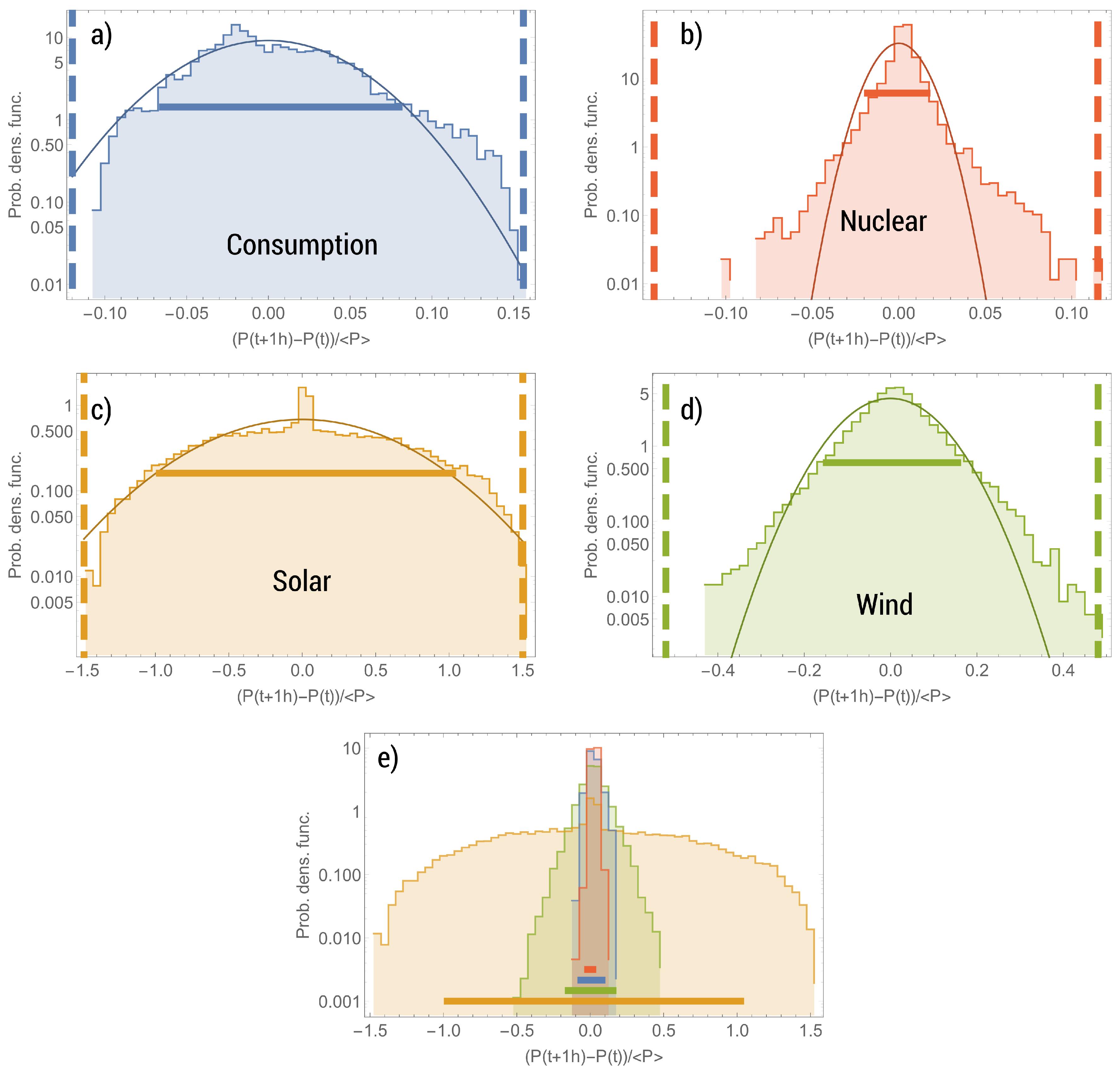
3.1. Relative Power Differences at 1 h

Let us first consider the power variations between a given time and 1 h later—this duration is arbitrarily chosen and the general case is considered in Section 3.2.

The year 2018 counts 17,520 30-min intervals; i.e., 17,518 pairs of points $\left(P\left(t\right),P(t+1\mathrm{h})\right)$. Among these pairs, we remove those corresponding to zero power: a long period of null production should not be confused with a range of stability. In Figure 1, we show the probability density function for the yearly distribution of $\frac{P(t+1\mathrm{h})-P\left(t\right)}{〈P〉}$, which gives the relative number of times the production has changed by a given factor. In order to quantify the spread of these relative variations, we consider, for example, the interval between the 5th and 95th percentiles of the distribution; that is, the span in which 90% of the deviations are encompassed (represented by a solid horizontal bar on the graphs). If this choice is arbitrary, the conclusions remain identical for all intervals. Extreme deviations, which occur at least once a year, are also shown (dashed vertical lines in the figure).

The first considered quantity is consumption, which we use as a standard for defining whether a source is intermittent or persistent. It appears that the typical order of magnitude of the consumption relative variations over 1 h is a factor ~$\pm 7\%$ (i.e., 10% of the time, power demand changes by more than 7% of the average demand within the following hour), while extreme values reach ~$\pm 15\%$. Note that the distribution is skewed towards positive values, meaning that the consumption seems to increase more importantly within one hour than it decreases.

The distribution of the nuclear sector is much narrower than that of consumption, with a typical factor $\pm 1.5\%$ and an extreme of $\pm 12\%$. Importantly, the distribution appears as strongly non-Gaussian: the distribution is strongly peaked, while at the same time larger variations occur much more frequently than what could be expected from a normal law with the same standard deviation; its kurtosis (fourth-order moment) is indeed ~16. This observation highlights again the complex nature of power series, which cannot be reduced to simple statistical distributions.

Wind production is regularly modified by a factor $\pm 15\%$ corresponding to the most extreme variations of power demand, which classify the wind sector as intermittent. Furthermore, extreme variations can reach $\pm 50\%$ of the average wind production over a period of 1 h, exemplifying the non-Gaussian behavior of the distribution with a kurtosis ~5.

Because of its cancellations at the beginning and at the end of the day, PV production is experiencing important variations, far beyond that of consumption. It should, however, be noted that the indicator exhibits at least two contributions: meteorological variability and day/night alternation. The latter is perfectly predictable, and constitutes the major part of the PV intermittency. The influence of meteorological variability is examined in the next subsection.

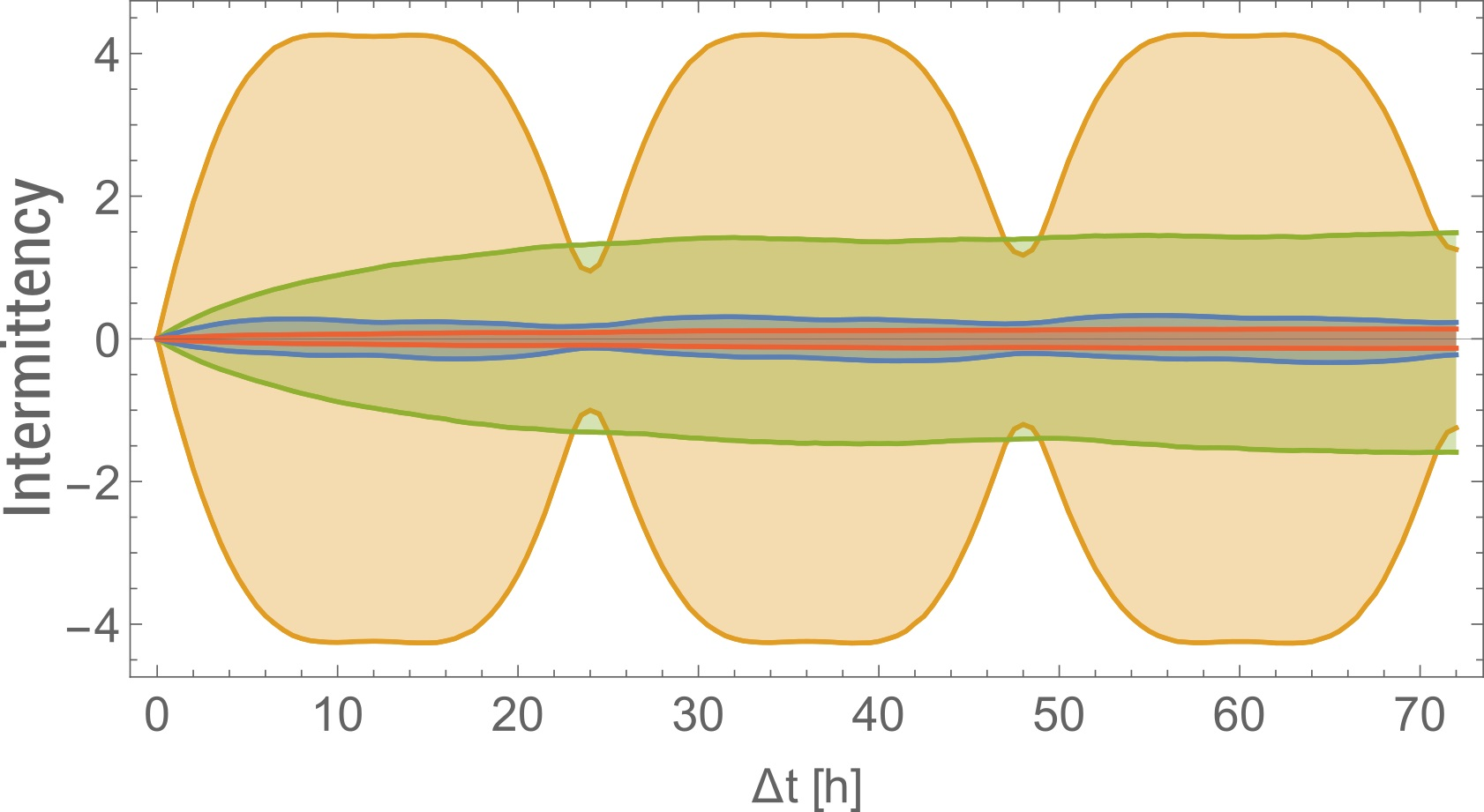
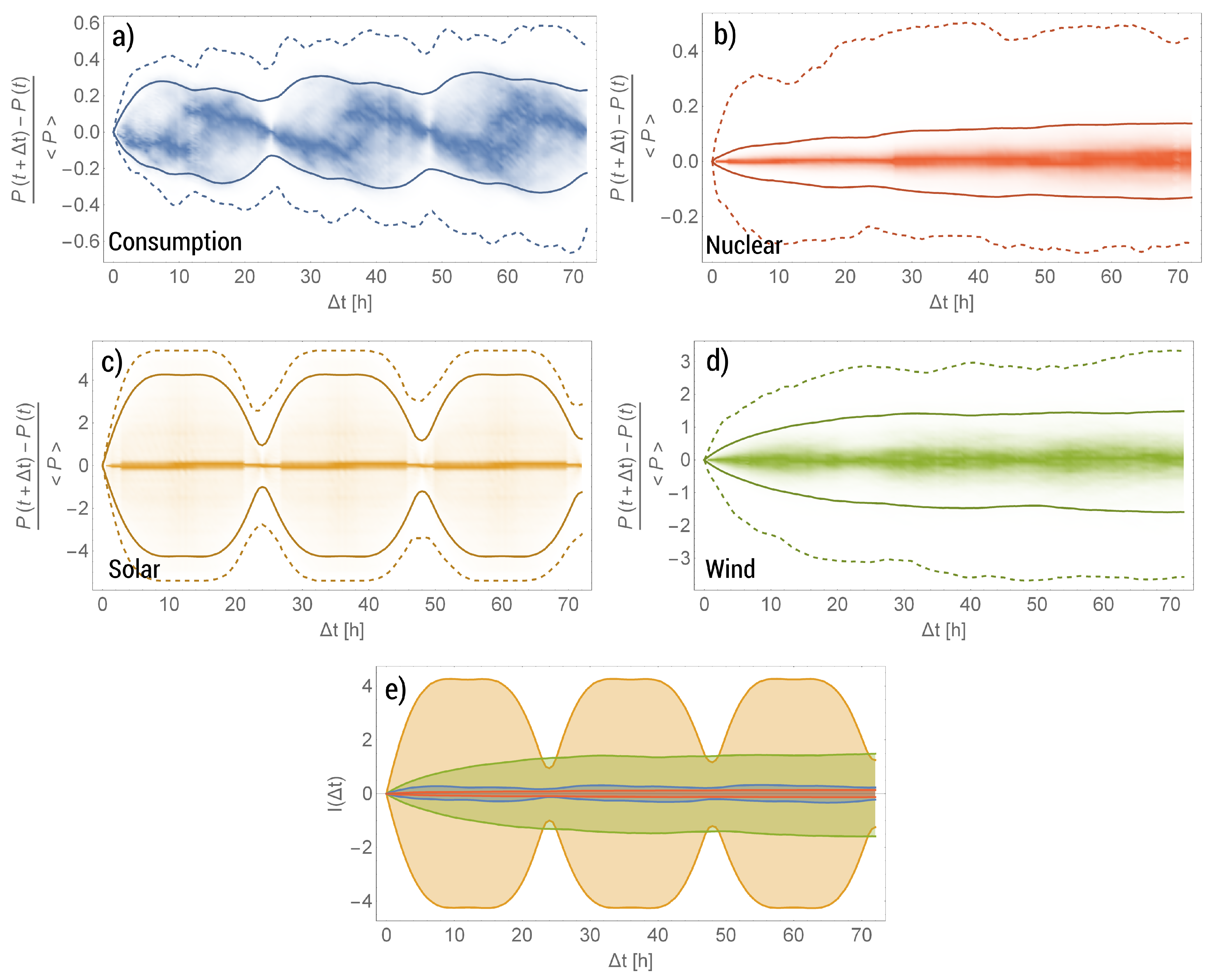
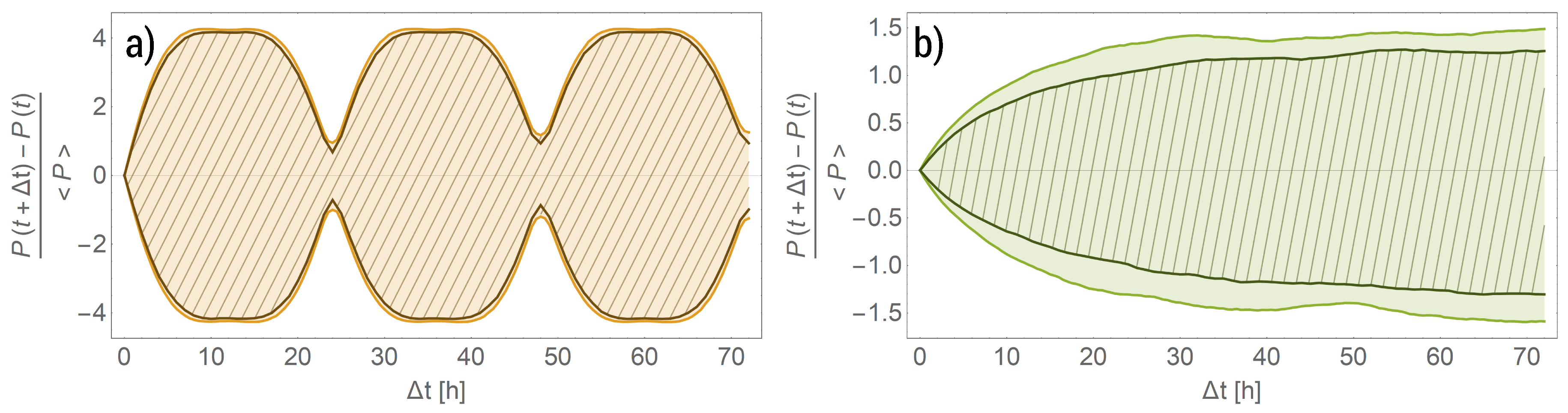
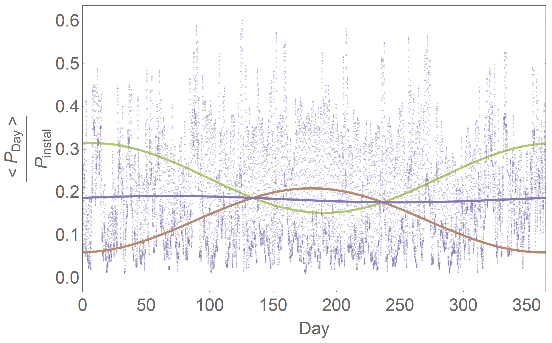
3.2. Intermittency as a Function of Time

The previous choice of comparing powers within the following hour is arbitrary, but it is a graphic way to introduce the inter-percentile gap and the extreme values as relevant indicators to account for the variation distributions of the sectors at stake. In this section, we are interested in the temporal behavior of these quantities, as indicators of the intermittency of each sector.

For each interval $\Delta t$ lesser than three days, the power deviation $\frac{P(t+\Delta t)-P\left(t\right)}{〈P〉}$ is evaluated at each time t using the same method as in the previous section. Figure 2 shows the evolution of the indicator for intermittency $I(\Delta t)$ estimated as the inter-percentile gap and the extreme values of the relative variations of each sector:

$$\begin{array}{c}\hfill I(\Delta t)={\mathrm{interpercentile}}_{5;95}\left(\left\{\frac{P(t+\Delta t)-P\left(t\right)}{〈P〉}\right\}\right)\end{array}$$

Note that the probability density function is represented through shading density, implying that the mode of the distribution is represented by the darkest point. This figure offers a quantitative visualization of intrinsic intermittency and constitutes the main contribution of this work. Several conclusions can be drawn from this.

First, the classification of PV and wind among intermittent sources, and of nuclear among the non-intermittent or persistent, is verified for all available durations. Indeed, for all time spans $30\min \le \Delta t\le 72\mathrm{h}$ and regardless of the method chosen to quantify the spread of the variations distribution, consumption intermittency is greater than that of nuclear production but smaller than those of wind and solar (see Figure 2, bottom).

Secondly, it is possible to observe a saturation of the indicator for intermittency, which is particularly clear for the nuclear and wind sectors: between a given time t and a later time $t+\Delta t$, the width of the distribution of the relative power variations increases rapidly with $\Delta t$, and then becomes stationary beyond a duration $\Delta t\simeq 10\mathrm{h}$. This phenomenon indicates that the uncertainty on the variation of the produced power does not increase anymore beyond this time (over a few days).

Conversely, it is interesting to note that the relative variations of consumption and PV production show a periodic modulation of 24 h due to the daily cycle (which adds up to the saturation mentioned above). For the PV sector, the intermittency at 24 h indicates the weather variations mentioned above: between t and $t+24\mathrm{h}$, the position of the Sun in the sky is almost unchanged and the observed deviations are mainly due to meteorological conditions. We stress again that the small values at $\Delta t=24\mathrm{h}$ do not display a lower production at a specific time, but a stronger correlation of the production between t and $t+24\mathrm{h}$. It appears then that, beyond the daily cycles, the PV intermittency due to meteorological conditions is smaller than that of the wind sector (see Figure 2, bottom). Should this feature be removed, through energy storage or other compensation systems, the PV production would possibly be less intermittent than the wind one, while both remain significantly more so than consumption or nuclear. It should be noted, however, that this analysis does not make it possible to assess the impacts of rapid changes in these conditions (such as clouds), but only their average influences from one day to the next.

Remarkably, the consumption shows a dissymetric distribution at almost all intervals $\Delta t$, following the behavior noted in the previous section. Indeed, the skewness at $\Delta t=1\mathrm{h}$, towards positive values, grows stronger up to $\Delta t=12\mathrm{h}$, as can be seen by the spread between the mode (darker part of the distribution in Figure 2, top left) and the 95th percentile (solid line); then, the skewness declines towards a symmetric distribution at $\Delta t=24\mathrm{h}$, from the negative values. This results from time asymmetry in the consumption profile: peaked increase and slower decrease for $30\min \le \Delta t\le 12\mathrm{h}$, slow increase and stronger decrease for $12\mathrm{h}\le \Delta t\le 24\mathrm{h}$. Finally, one can also note the sharp peak of the PV distribution, clearly visible for the 1 h variations in Figure 1 and represented in Figure 2 by shading density for all intervals $30\min \le \Delta t\le 72\mathrm{h}$; thus, it is visible via the thin darker line around $I(\Delta t)=0$.

4. Discussion

Two approaches are often considered to limit the intermittent behavior of a source: aggregation and complementarity of production sources. As an application of the definition presented above, this section quantifies the impacts of these approaches, using the 5th–95th percentile interval only in the following analyses.

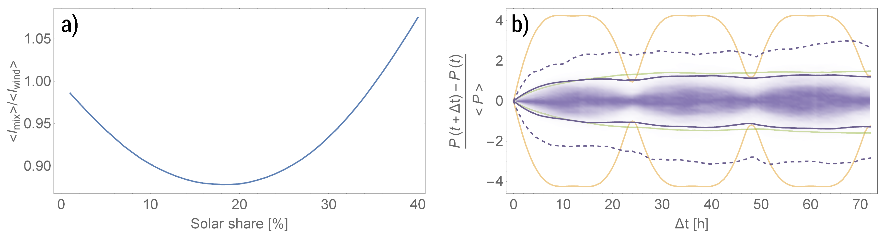
4.1. Impact of Aggregation

Aggregation consists of multiplying the sources of fluctuations to mitigate their effects: an installation may undergo certain variations (due to breakdowns, meteorological conditions, etc.) which largely affect its production, but these individual hazards are smoothed out when a large number of identical installations is considered [33]. This argument is often summarized as, “the wind is always blowing somewhere,” or “the Sun is always shining somewhere,” implying that the intermittency of power production could disappear if a large enough area is considered. However, quantitative analysis performed on the autocorrelation function [34] or on the load factor [35] of wind power production in Western Europe showed that the influence of aggregation can be quite limited. It is therefore relevant to consider the quantitative analysis of intermittency devised above.

To illustrate this idea, Figure 3 compares the intermittency, as the 5–95th percentile interval of the distribution, for productions in France only and for aggregated productions in France and Germany, using data from the European Network of Transmission System Operators for Electricity (ENSTO-E) transparency platform [36].

The intermittency of PV production comes mostly from day–night alternation, which is not mitigated by the shift from the national level to the supranational scale. The intermittency at 24 h, which mostly depends on weather conditions, remains much larger than that of consumption, despite a small decrease thanks to the upscaling. For the PV sector, aggregation has thus a minor effect on intermittency as defined herein. The wind sector shows a clearer gain in persistency due to the aggregation, and illustrates well the principle at work: averaged over a wider territory, the variations of wind and therefore of wind power production are less important in relative values. Nevertheless, we recover with our method the results of the aforementioned works and conclude that the aggregated wind production remains intermittent as compared to consumption. It should, however, be noted that the current deployment of wind farming is not optimized to reduce intermittency, but rather to maximize production, and that aggregation could certainly further improve the persistency of production in a deployment informed by weather regimes [37].

4.2. Impact of Complementarity

The complementarity between wind and PV productions is often considered to ease their introduction into the energy mix, as they are relatively well anti-correlated at long time scales (see Figure 4, solid lines). However, if this complementarity allows for a significant smoothing of seasonal productions, it is insufficient to compensate for the rapid daily variations in production (see Figure 4, data points) and a quantitative evaluation of the intermittency of the mix remains essential.

To do so, we compute the intermittency indicator $I_{\mathrm{mix}}(\Delta t)$, as the 5–95th percentile interval, for a production mixing solar and wind productions, and we estimate the fraction of PV production to minimize the average value of $I_{\mathrm{mix}}$ (see Figure 5). We find numerically that least intermittent mix, at the time scale considered here (a few days), consists in ∼20% of PV sources and ∼80% of wind sources, far from the 50–50 distribution usually pictured (see Figure 4). Indeed, the addition of a small amount of PV production reduces slightly the intermittency as compared to a pure wind production, but a more significant contribution from solar sources increases the intermittency due to the strong variations induced by the day–night cycle.

We note that the criterion chosen for this study (minimization of the intermittency over 72 h) is arbitrary and lays the focus on middle term fluctuations. It is also possible to rather highlight longer term behaviors by minimizing the saturation value (in which case the optimal mix features ∼25% of PV sources) or to stress instead shorter time scales by minimizing $I_{\mathrm{mix}}(\Delta t_0)$, where $\Delta t_0$ is the smallest time step available in the data (for $\Delta t_0=30$ min as is the case with RTE data, the optimal mix features ∼8% of PV sources). In all cases, it appears that solar sources can decrease the intermittency of the mix but should be restrained to low fraction of the total production if the intermittency is to be minimized.

The situation is likely to be reversed if a significant storage capacity is considered. Indeed, as mentioned before, the intermittency of PV production reduces below that of wind sources at $\Delta t\simeq 24\mathrm{h}$ when the influence of the day–night cycle is removed. It is therefore likely that if solar production can be averaged over a 24 h time-scale, the optimal mix would feature a majority of PV sources and a minority of wind power. However, detailed modeling of the storage strategy would be required to go beyond this qualitative analysis.

5. Conclusions

In this work, we suggested an intrinsic definition of the indicator for intermittency as the spread of the power variations (relative to the average power) between a given instant and a subsequent instant. An electricity production source can therefore be described as intermittent when its indicator for intermittency is larger than that of the consumption, which serves as a reference. This definition, based on power time series, does not differentiate between driven and intrinsic intermittency and should be distinguished from notions of dispatchability, predictability and variability. Applied to the maximum production capacity of a large enough sector, it characterizes it intrinsically, independently of the current installed capacity, technology efficiency or current state of the energy mix.

We applied this approach to the electricity power in France, and studied the intermittency of the solar, wind and nuclear sectors. In view of this methodology, solar and wind productions appear intermittent, unlike nuclear production, which is more persistent than consumption. The non-Gaussian behavior of the distributions indicates that extreme variations (that is, variations much larger than the standard deviation) occur much more often than what could be expected from a normal law. We used our definition and analysis to discuss two methods routinely invoked to deal with intermittency. We found that the influence of aggregation is not straightforward, and not sufficient in the case considered to mitigate the intermittent nature of solar or wind sources.

While providing insights on intermittency mitigation, the intrinsic perspective adopted in this paper does not provide operational tools for network management: a large value of the indicator for intermittency is not sufficient to disqualify a source, nor is persistency (that is, a small value of $I(\Delta t)$) sufficient to justify the presence of a source in the energy mix. Rather, our approach is intended to offer quantitative tools when comparing intermittency of different sources, or mixes. Even though the construction of a dedicated definition necessarily requires arbitrary choices, we believe that this work has a general scope, as it clearly distinguishes intermittency from related notions and underlines the physical meaning of each concept. Lifting this ambiguity is certainly not sufficient to reconcile the debate, but contributes to underlining the difference between a physical property (characterizing an energy production), a management strategy (mitigating the physical constraints of the production) and an energy policy (selecting a management strategy). Doing so, we hope to defuse the concept of intermittency from the ideological load it has acquired, and offer a common ground for future discussions, especially regarding large integration of renewable sources in the energy mix.

References

1. IRENA. Renewable Capacity Statistics 2019; Technical Report 978-92-9260-123-2; IRENA: Abu Dhabi, UAE, 2019. [Google Scholar]
2. International Energy Agency. Getting Wind and Sun onto the Grid, a Manual for Policy Makers; International Energy Agency: Paris, France, 2017. [Google Scholar]
3. Heptonstall, P.; Gross, R.; Steiner, F. The Costs and Impacts of Intermittency, 2016 Update; UK Energy Research Center: London, UK, 2017. [Google Scholar]
4. Wagner, F. Electricity by intermittent sources: An analysis based on the German situation 2012. Eur. Phys. J. Plus 2014, 129. [Google Scholar] [CrossRef] [Green Version]
5. Clack, C.T.M.; Qvist, S.A.; Apt, J.; Bazilian, M.; Brandt, A.R.; Caldeira, K.; Davis, S.J.; Diakov, V.; Handschy, M.A.; Hines, P.D.H.; et al. Evaluation of a proposal for reliable low-cost grid power with 100% wind, water, and solar. Proc. Natl. Acad. Sci. USA 2017, 114, 6722–6727. [Google Scholar] [CrossRef] [PubMed] [Green Version]
6. Heard, B.; Brook, B.; Wigley, T.; Bradshaw, C. Burden of proof: A comprehensive review of the feasibility of 100% renewable-electricity systems. Renew. Sustain. Energy Rev. 2017, 76, 1122–1133. [Google Scholar] [CrossRef]
7. Budischak, C.; Sewell, D.; Thomson, H.; Mach, L.; Veron, D.E.; Kempton, W. Cost-minimized combinations of wind power, solar power and electrochemical storage, powering the grid up to 99.9% of the time. J. Power Sources 2013, 225, 60–74. [Google Scholar] [CrossRef] [Green Version]
8. Jacobson, M.Z.; Delucchi, M.A.; Cameron, M.A.; Frew, B.A. Low-cost solution to the grid reliability problem with 100% penetration of intermittent wind, water, and solar for all purposes. Proc. Natl. Acad. Sci. USA 2015, 112, 15060–15065. [Google Scholar] [CrossRef] [PubMed] [Green Version]
9. Milborrow, D. Wind Power on the Grid. In Renewable Electricity and the Grid, the Challenge of Variability; Boyle, G., Ed.; Earthscan: London, UK, 2007. [Google Scholar]
10. Lovins, A.B.; Sheikh, I.; Markevich, A. Nuclear power: Climate fix or folly? In The Energy Reader; Nader, L., Ed.; John Wiley & Sons: Hoboken, NJ, USA, 2010. [Google Scholar]
11. Inhaber, H. Why wind power does not deliver the expected emissions reductions. Renew. Sustain. Energy Rev. 2011, 15, 2557–2562. [Google Scholar] [CrossRef]
12. Linnemann, T.; Vallana, G.S. Wind energy in Germany and Europe. Pt. 2. Status, potentials and challenges for baseload application: European situation in 2017. Atw. Int. Z. Kernenerg. 2019, 64, 141–148. [Google Scholar]
13. MacKay, D. Sustainable Energy—Without the Hot Air; UIT Cambridge Ltd.: Cambridge, UK, 2009; p. 384. [Google Scholar]
14. Négawatt, A. Are Renewable Energy Sources Intermittent? 2016. Available online: https://decrypterlenergie.org/les-energies-renouvelables-sont-elles-intermittentes-2 (accessed on 25 June 2020).
15. Association “Save the Climate”. Wind and Solar Electricity Production, CO2 Emission and Cost of Electricity for Households in Western Europe. 2017. Available online: https://www.sauvonsleclimat.org/fr/base-documentaire/electricite-renouvelable-intermittente-europe (accessed on 25 June 2020).
16. Greenpeace France. Electricity Market: Who Are the Greener Electricity Providers? Technical Report. 2018. Available online: https://www.guide-electricite-verte.fr/wp-content/uploads/sites/9/2018/09/Guide-electriciteverte-2018-Methodologie-Greenpeace-France.pdf (accessed on 10 October 2018). See also: https://www.liberation.fr/checknews/2018/10/05/selon-greenpeace-le-nucleaire-emet-plus-deco2-que-le-photovoltaique-est-ce-vrai_1682628 (accessed on 25 June 2020) .
17. Tarroja, B.; Mueller, F.; Eichman, J.D.; Samuelsen, S. Metrics for evaluating the impacts of intermittent renewable generation on utility load-balancing. Energy 2012, 42, 546–562. [Google Scholar] [CrossRef]
18. Chang, M.K.; Eichman, J.D.; Mueller, F.; Samuelsen, S. Buffering intermittent renewable power with hydroelectric generation: A case study in California. Appl. Energy 2013, 112, 1–11. [Google Scholar] [CrossRef]
19. Gutierrez-Martín, F.; Da Silva Alvarez, R.; Montoro-Pintado, P. Effects of wind intermittency on reduction of CO2 emissions: The case of the Spanish power system. Energy 2013, 61, 108–117. [Google Scholar] [CrossRef]
20. Réseau Transport Electricité (French Electricity Transmission Network). Definitive and Consolidated Domestic eCO2-Mix Data. 2018. Available online: https://www.rte-france.com/en/eco2mix/eco2mix-telechargement-en (accessed on 25 June 2020).
21. French Ministry for the Economy and Finance. Loi 2000-108 du 10 Février 2000 Relative à la Modernisation et au Développement du Service Public de l’électricité (ECOX 9800166L); French Ministry for the Economy and Finance: Paris, France, 2016. [Google Scholar]
22. Coker, P.; Barlow, J.; Cockerill, T.; Shipworth, D. Measuring significant variability characteristics: An assessment of three UK renewables. Renew. Energy 2013, 53, 111–120. [Google Scholar] [CrossRef]
23. Ren, G.; Liu, J.; Wan, J.; Guo, Y.; Yu, D.; Liu, J. Measurement and statistical analysis of wind speed intermittency. Energy 2017, 118, 632–643. [Google Scholar] [CrossRef]
24. Sinden, G. Characteristics of the UK wind resource: Long-term patterns and relationship to electricity demand. Energy Policy 2007, 35, 112–127. [Google Scholar] [CrossRef]
25. Masters, G.M. Renewable and Efficient Electric Power Systems; John Wiley & Sons Inc.: Hoboken, NJ, USA, 2013. [Google Scholar]
26. Wilks, D.S. Statistical Methods in the Atmospheric Sciences; International Geophysics Series; Elsevier: Amsterdam, The Netherlands; Academic Press: Cambridge, MA, USA, 2011. [Google Scholar]
27. Apt, J. The spectrum of power from wind turbines. J. Power Sources 2007, 169, 369–374. [Google Scholar] [CrossRef]
28. Van der Hoven, I. Power spectrum of the horizontal wind speed in the frequency range from 0.0007 to 900 cycles per hour. J. Meteor. 1957, 14, 160–164. [Google Scholar] [CrossRef] [Green Version]
29. Tarroja, B.; Mueller, F.; Eichman, J.D.; Brouwer, J.; Samuelsen, S. Spatial and temporal analysis of electric wind generation intermittency and dynamics. Renew. Energy 2011, 36, 3424–3432. [Google Scholar] [CrossRef] [Green Version]
30. Ghashghaie, S.; Breymann, W.; Peinke, J.; Talkner, P.; Dodge, Y. Turbulent cascades in foreign exchange markets. Nature 1996, 381, 767–770. [Google Scholar] [CrossRef]
31. Morales, A.; Wachter, M.; Peinke, J. Characterization of wind turbulence by higher-order statistics: Characterization of atmospheric turbulence. Wind Energy 2012, 15, 391–406. [Google Scholar] [CrossRef]
32. Anvari, M.; Lohmann, G.; Wächter, M.; Milan, P.; Lorenz, E.; Heinemann, D.; Tabar, M.R.R.; Peinke, J. Short term fluctuations of wind and solar power systems. New J. Phys. 2016, 18, 063027. [Google Scholar] [CrossRef]
33. Kiviluoma, J.; Holttinen, H.; Weir, D.; Scharff, R.; Söder, L.; Menemenlis, N.; Cutululis, N.A.; Danti Lopez, I.; Lannoye, E.; Estanqueiro, A.; et al. Variability in large-scale wind power generation. Wind Energy 2016, 19, 1649–1665. [Google Scholar] [CrossRef] [Green Version]
34. Livet, F. The Problem of Intermittency of Renewable Energies: Solar and Wind Energy; Technical Report INIS-FR–14-0410; IAEA-INIS: Vienna, Austria, 2011. [Google Scholar]
35. Flocard, H.; Pervès, J.P.; Hulot, J.P. Electricité: Intermittence et foisonnement des énergies renouvelables. Techniques de l’Ingénieur 2014, 202, BE8586. [Google Scholar]
36. European Network of Transmission System Operators for Electricity Transparency Platform. Actual Generation per Production Type. 2018. Available online: https://transparency.entsoe.eu/ (accessed on 25 June 2020).
37. Grams, C.M.; Beerli, R.; Pfenninger, S.; Staffell, I.; Wernli, H. Balancing Europe wind-power output through spatial deployment informed by weather regimes. Nat. Clim. Chang. 2017, 7, 557–562. [Google Scholar] [CrossRef] [PubMed] [Green Version]
Figure 1. Histogram of the relative variations of the instantaneous power over 1 h: P ( t + 1 h ) P ( t ) / P . (a) consumption (blue); (b) nuclear (red); (c) solar photovoltaic (PV) (yellow); (d) wind (green). Solid lines show a Gaussian distribution with the same standard deviation for comparison. Dashed vertical lines indicate the minimum and maximum values. The horizontal bar marks the interval between the 5th and 95th percentiles, where 90% of the events occur, which will be used to quantify the spread of the distribution in the next section. The last figure (e) shows the same data with the same sampling for all four sectors in order to ease the comparison.
Energies 13 03366 g001
Figure 2. Indicator for intermittency over time. (a) consumption (blue); (b) nuclear (red); (c) solar photovoltaic (PV) (yellow); (d) wind (green). The solid lines correspond to I ( Δ t ) as defined here, that is, the 5th and 95th percentiles where 90% of the most central points lie (see horizontal bar in Figure 1). The dashed lines give the extreme variations (see dashed vertical lines in Figure 1). The shading intensity at each point is proportional to the probability density function at this point (the darkest region corresponding to the mode), so that a slice at a given Δ t is a “top view” of the corresponding histogram, as presented in Figure 1. The last figure (e) combines the previous figures to ease comparisons. Let us recall that, despite a possible resemblance to the daily power profiles, we display here the variations of consumption at all instants t of the year, and for a variable Δ t . The relatively small inter-percentile interval of consumption at Δ t 24 h , for example, has no connection with the fact that consumption is low at t 24 h (midnight).
Energies 13 03366 g002
Figure 3. Indicator for intermittency of (a) PV (yellow) and (b) wind (green), in France (colored area) and France + Germany (hatched area).
Energies 13 03366 g003
Figure 4. Solid line: daily averaged capacity factor of PV (orange) and wind (green) productions and of a 50–50 mix (purple) throughout the year. Data points: instant value of the 50–50 mix.
Energies 13 03366 g004
Figure 5. (a): Normalized averaged value of I mix ( Δ t ) for Δ t varying between 0 h and 72 h as a function of the PV fraction in the solar-wind mix. (b): Indicator for intermittency for a mix with 0% (green), 20% (purple) and 100% (yellow) of PV.
Energies 13 03366 g005