Non-Cooperative Game in Block Bidding Markets Considering Demand Response

Abstract

With the reform of electricity markets, demand response (DR) plays an important role in providing flexibility to the markets. Block bidding market is a new market mode, which is based on the concept of “the same quality, the same price”. The mechanism has great effects in reducing start-stop related costs. In this paper, we propose a double-sided non-cooperative game model in block bidding markets with a DR program. The model combines the advantages of block bidding and the simplicity of hourly bidding. In the model, one side is the non-cooperative game of supply-side power firms, and we propose a novel supply function bidding model based on block duration and load capacity to maximize each firm’s profit. The other side is the demand-side different types of customers, and we propose a DR model that combines hourly-various prices with the block bidding mechanism to maximize each customer’s payoff. The overall market optimization problem is solved by a distributed iterative algorithm, which has great convergence performance. We verify the proposed model on real data, and the results show that the demand load curve becomes flattened with DR, and the total generation costs decrease while the social welfare is significantly improved.

1. Introduction

Electricity market reforms optimize power resources allocation and reduce energy costs by introducing competition to the market [1,2,3]. In the open electricity markets, power supply firms submit bids to compete with each other, and customers participate in demand response (DR) in order to reduce the power purchase costs.

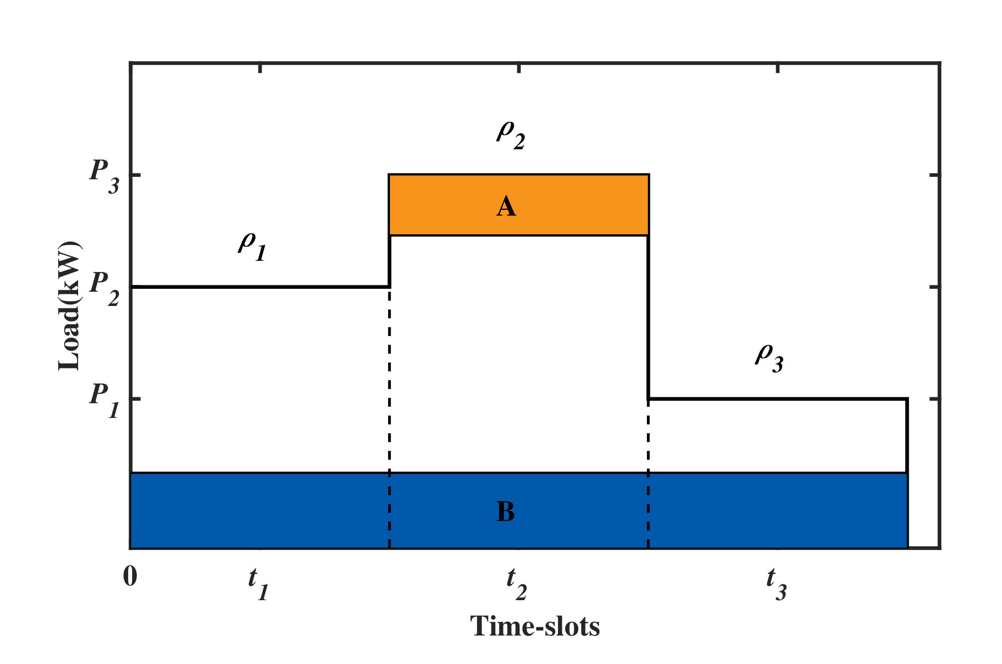
Block bidding is a new market bidding mechanism. The basis of block bidding markets is the concept of “the same quality, the same price” [4]. Figure 1 shows the comparison of hourly bidding mode and block bidding mode. A and B represent two power supply firms. In hourly bidding markets, firms submit bids for each time-slot, and the electricity prices at $t_1$, $t_2$, and $t_3$ are, respectively, ${\rho }_1$, ${\rho }_2$, and ${\rho }_3$. However, firm A is running at peak load and firm B is running at base load; their generation costs are quite different. It is unfair for both of them to sell electricity at the same price of ${\rho }_2$ in time-slot $t_2$. Therefore, block bidding mode is put forward to solve this problem. The new mode allows firms to submit bids for each block, and each block is traded at the same price. Generally, the division of blocks is based on the block duration. That is to say, firm B submits bid for the blue block, and the block should be traded at the same price. When compared with the hourly bidding mode, block bidding mode can help to reduce the start-stop related generation costs [5], and especially effective in countries or regions with large amounts of thermal power generation.

DR is a powerful tool for increasing market flexibility and decreasing energy costs. By customers’ participation in DR, the market demand curve can achieve peak shaving and valley filling effects [6,7,8]. Power supply firms’ competition and customers’ DR can be considered as non-cooperative games. In a non-cooperative game, each player optimizes his/her own strategy to maximize his/her utility, when considering that other players’ strategies are fixed. The non-cooperative game will eventually converge to a solution, which is known as Nash equilibrium [9]. In recent years, researching DR in competitive electricity markets from the perspective of game theory has become an important topic. On this issue, researches have been carried out on two different focuses.

One focus is the optimal bidding strategy of the power supply side, based on different market mechanisms: block bidding or hourly bidding. Shah et al. [10] studied the Flexi type block bid in Nord Pool and proposed an optimal placing model of block bid execution time based on social welfare maximization. In Nord Pool, a block bid can only be accepted if its price is not higher than the average market price. Zak et al. [11] considered that there is a dilemma in such market rules, because block bids selection as a primal solution cannot be properly exercised without knowing the prices as a dual solution. Therefore, they proposed a model harmonizing such complex “primal-dual” market rules. Ajay et al. [12] proposed a profit maximization model for generators under block bidding rules and let each supplier use a probability distribution function for predicting the bidding prices of rivals. Unlike the complex and single form of block bidding, the hourly bidding mechanism has developed for a long time, and the bidding method is relatively flexible. Kamyab et al. [13] employed a supply function bidding mechanism that was based on an hourly bidding rule to model the utility firms’ profit maximization problem. Chai et al. [14] proposed a two-level non-cooperative game model, that each utility firm determines its generation amount and power price at each time-slot, and each customer chooses a firm to buy electricity. However, the existing block clearing rules in [10,11] use the price of hourly markets to settle block orders, which is complex and cannot fully reflect the advantages of block bidding, and the supply-side models do not consider firms’ generation costs and profits. Although Ref. [12] takes utility firms’ profit into consideration, the prediction model of rivals’ block bidding price is rough and lacks demand-side feedback. Researches [13] and [14] are based on the hourly bidding mechanism, and they cannot reflect the relationship between block duration and generation costs, which are not applicable for block bidding markets.

The other focus in competitive electricity markets is the demand-side DR program, which is based on cooperative or non-cooperative game theory. Elghitani et al. [15] proposed a method for residential demand aggregation to minimize the total consumption costs, based on a multi-class demand loads queuing system. Guo et al. [16] proposed an optimal pricing strategy for retailers to maximize its profit and an optimal DR resources scheduling model for minimizing customers’ total electricity purchase costs, based on the block trading mode. Sanchez de la Nieta et al. [17] modeled demand-side management as flexible block orders, and the market-clearing algorithm decides the accepted order according to the principle of social welfare maximization. Motalleb et al. [18] modeled the competitive behavior among DR aggregators for selling excess energy in storage devices directly to other aggregators in a power market. Khanna et al. [19] described a price-based DR methodology for the application of complete households incorporating key DR features, such as an electric vehicle and some smart residential appliances. However, most researches are based on cooperative game theory, such as [15,16,17], which rely on an aggregator or a third-party algorithm to optimize customers’ load resources. Besides, the widely known block orders in [17] is difficult for small scale residential customers to participate in. As for Refs. [18,19] based on the non-cooperative game theory, Ref. [18] is not applicable for customers without storage devices. Although Ref. [19] allows each customer to optimize its own demand loads through smart residential appliances, the mechanism is based on hourly-various prices.

In this paper, we improve the competitive block bidding market model on the above two focuses. On the optimal bidding strategy of the supply-side, we consider the advantages of block bidding and propose a supply curve bidding mechanism in block bidding markets. On the demand-side, we convert the block electricity price into the hourly price in order to meet the needs of different customers, and then propose a distributed demand-side model that combines block bidding markets into the hourly DR model. The whole electricity market is modeled as a double-sided non-cooperative game, which is composed of the supply-side game and the demand-side game. The main contributions can be summarized, as follows:

• A novel supply function bidding model that is based on block duration and load capacity in block bidding markets, which realizes profit maximization of power supply firms and supply-demand balance at each time-slot.
• A DR model in block bidding markets with hourly-various prices based on fixed load and shiftable load resources, which maximizes each customers’ daily payoff. The model combines the advantages of block bidding markets and hourly bidding markets, and it has great peak shaving effects.
• A distributed market architecture and distributed iterative algorithm in block bidding markets, which can guarantee the double-sided non-cooperative game converge to the Nash equilibrium within limited iteration and time.

The rest of this paper is organized, as follows. The mathematical model of the double-sided non-cooperative game in block bidding markets is introduced in Section 2. Solution approach of the distributed iterative algorithm is presented in Section 3. The simulation results and analysis of the proposed model effects are shown in Section 4. Section 5 describes the conclusion and future works.

2. Mathematical Model

In this section, we propose a double-sided non-cooperative game model, which composed of a block-based supply-side game and a time-based demand-side game. The architecture of the market model is illustrated first. The detailed mathematical models of the supply-side and demand-side game follows.

2.1. Market Model

2.1.1. Architecture of the Double-Sided Game

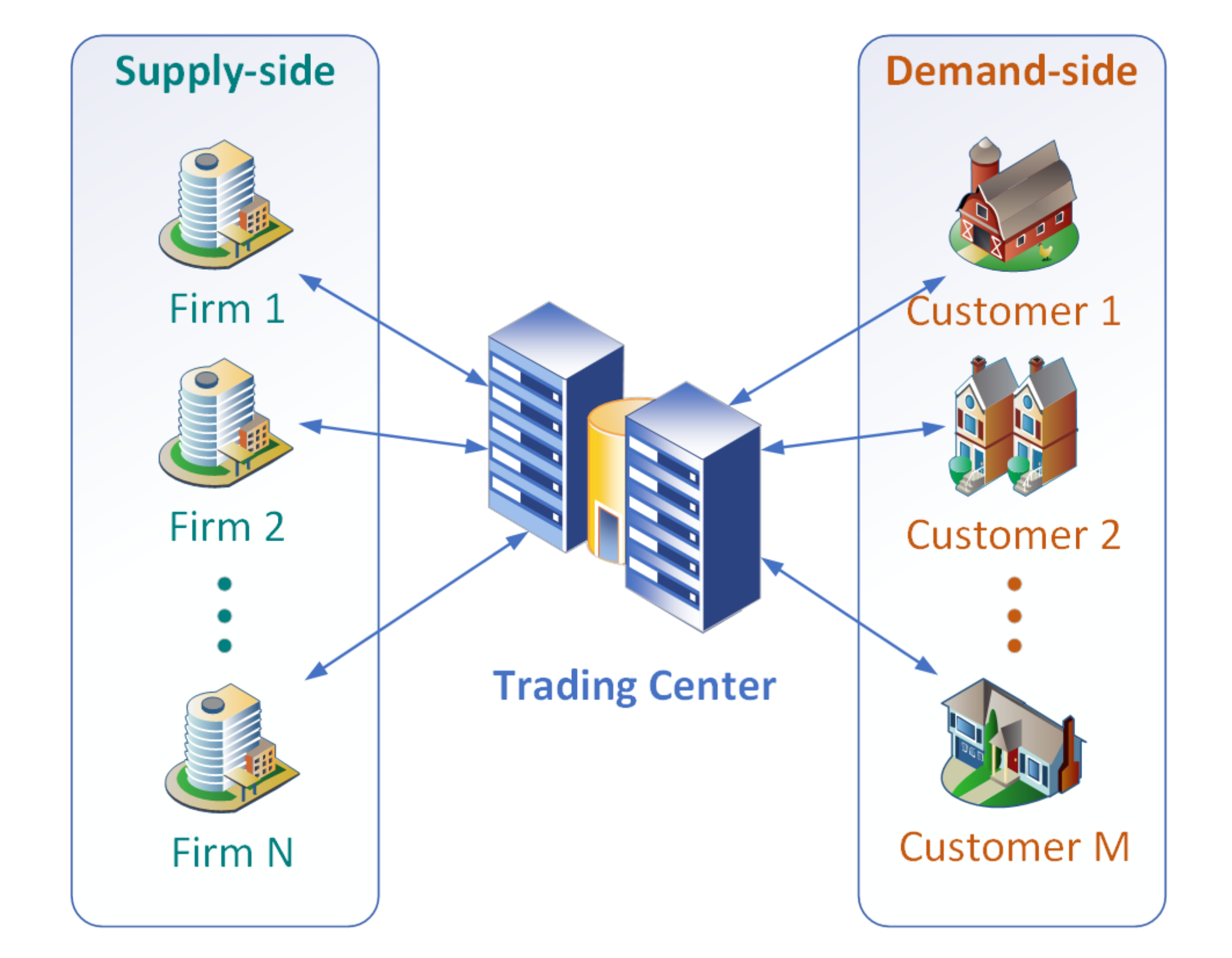
Suppose that there are N firms and M customers in the market. Customers can be residents, companies, or retailers. A trading day is divided into T time slots. Let $\mathcal{T}=\{1,2,\dots ,t,\dots ,T\}$ denote the set of time slots. The architecture of the double-sided game is shown in Figure 2. The system is applied in the day-ahead block bidding markets. Firms and customers are interacted by the trading center. The trading center is non-profit and responsible for collecting demand and supply bid curves. The center also informs necessary market information to firms and customers. Transmission loss is not taken into consideration in this paper.

2.1.2. Trading Center for Block Bidding Markets

In block bidding markets, the demand load curve needs to be divided into several continuous blocks and traded at block-based prices. Therefore, the trading center is responsible for collecting customers’ demand curves and dividing the total load curve into blocks in order to inform each firm.

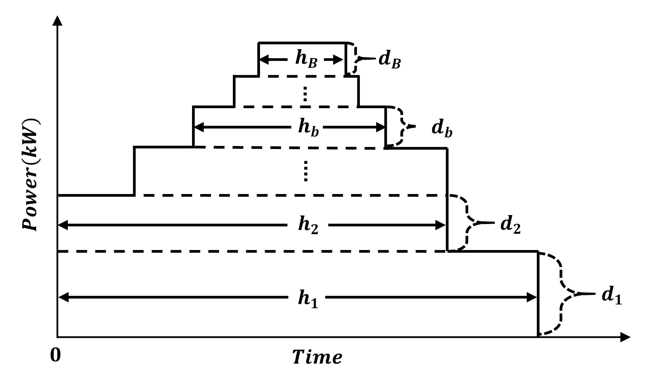
Assume the total power demands of each time-slot is $D_t$, define $\mathit{D}=\left(D_1,D_2,\cdots ,D_t,\cdots ,D_T\right)\in R^{1\times T}$ be the demand load curve vector. Let $\mathcal{B}=\{1,2,\dots ,b,\dots ,B\}$ denote the set of divided blocks, where b represents a block. Define $d_b$, $h_b$ be the power demand and duration for each block. Figure 3 shows the schematic diagram of block division in block bidding markets.

According to this figure, we can notice that there is a mapping from the demand load curve to the divided blocks. The mapping is defined as:

$$\mathrm{\Phi }:\mathit{D}\to \mathcal{B}$$

(1)

Then,

$$(d_b,h_b)=\mathrm{\Phi }\left(\mathit{D}\right)$$

(2)

We define two rules for grouping blocks:

• Duration-based rule. We group blocks based on their duration, and let ${\mathcal{B}}_h$ denote the set of blocks with duration h. Let $\mathcal{H}=\{1,2,\dots ,h,\dots ,H\}$ denote the set of blocks’ duration. Subsequently, the block set $\mathcal{B}$ can be described as $\mathcal{B}={\bigcup }_{h\in \mathcal{H}}{\mathcal{B}}_h$.
• Time-slot-based rule. We group load blocks based on their running time-slots, and let ${\mathcal{B}}_t$ denote the set of blocks running at t time-slot. Afterwards, $\mathcal{B}$ can be described as $\mathcal{B}={\bigcup }_{t\in \mathcal{T}}{\mathcal{B}}_t$.

In the double-sided game of block bidding markets, each firm submits bid for each block. However, it is difficult for residential and corporate customers to purchase electricity in blocks. On one hand, the power consumption of individual customers is not large and the electricity use time is scattered. On the other hand, it is not easy and efficient for residential or corporate customers to divide their load curves by themselves. We allow customers to trade in a traditional hourly mode in order to facilitate all types of customers to adjust their load curve. Accordingly, the trading center is responsible for transforming the block-based prices into time-based prices to inform customers. The block-based price is calculated by firms’ bids and customers’ demands. Let ${\gamma }_b$ be the block-based price of block b, and ${\gamma }_t$ be the time-based price of time-slot t. Subsequently, ${\gamma }_t$ can be expressed as the power weighted average price of blocks in ${\mathcal{B}}_t$:

$${\gamma }_t=\frac{{\sum }_{b\in {\mathcal{B}}_t}{d}_b{\gamma }_b}{D_t}\forall t\in \mathcal{T}$$

(3)

In a word, the trading center divides load curve into blocks and informs block information to each firm. Meanwhile, the trading center also calculates time-based prices to inform each customer. By the trading center, the block-based supply-side game and the time-based demand-side game are connected, reaching the balance of supply and demand.

2.2. Supply-Side Game

For power firms, especially those that mainly rely on thermal power, the generating cost is closely related to the running duration of units. Generally, a power station that runs longer can reduce more costs that are related to start and stop. If a unit can minimize the number of start-stops, then the average power generation cost will be greatly reduced. Therefore, in the non-cooperative supply-side game, we use the duration-based rule to group blocks and assume each firm submits a supply bid curve for each group. We assume each firm has no capacity limits and can provide energy that meets power demands with any h duration in set $\mathcal{H}$ according to the needs of customers.

Let $\mathcal{N}=\{1,2,\dots ,i,\dots ,N\}$ denote the set of firms, where i represents a firm. Let $q_{i,b}$ denote the supply amount of firm i for block b. Suppose the cost $C_{i,b}$ of each firm for each block is a strictly convex function of the supply amount $q_{i,b}$:

$$C_{i,b}\left(q_{i,b}\right)=\left(\frac{1}{2}{c}_{i,h}{q}_{i,b}^2+a_{i,h}{q}_{i,b}\right)h\forall b\in {\mathcal{B}}_h,h\in \mathcal{H},\forall i\in \mathcal{N}$$

(4)

where $c_{i,h}$ and $a_{i,h}$ are positive coefficients that are determined by the block duration h. Due to the fact that longer load duration within a day can get lower unit power generation costs, we set coefficients $c_{i,h}$ and $a_{i,h}$ be smaller values when the block duration h is longer.

The marginal cost $M{C}_{i,b}$ can be expressed as:

$$M{C}_{i,b}\left(q_{i,b}\right)=\left(c_{i,h}{q}_{i,b}+a_{i,h}\right)h\forall b\in {\mathcal{B}}_h,h\in \mathcal{H},\forall i\in \mathcal{N}$$

(5)

Based on the concept of “the same quality, the same price” in block bidding markets, firms do not need to submit bids for each block, but only submit bids that are based on different load duration. Define ${\beta }_{i,h}$ and ${\alpha }_{i,h}$ be the slope and intercept of the supply bid curve for h duration blocks, where ${\beta }_{i,h}>0$. It is assumed that the supply bid curve for each firm is an affine function of the block-based price ${\gamma }_b$:

$$q_{i,b}={\beta }_{i,h}({\gamma }_b-{\alpha }_{i,h})\forall b\in {\mathcal{B}}_h,\forall h\in \mathcal{H},\forall i\in \mathcal{N}$$

(6)

In this paper, we assume each firm submit ${\beta }_{i,h}$ of supply curve as strategic bids, and set ${\alpha }_{i,h}$ as pre-chosen values. The method is known as $\beta$-parameterization method in linear Supply Function Equilibrium (SFE) model [20]. Pre-chosen values of ${\alpha }_{i,h}$ can be set to the intercept $a_{i,h}$ of marginal cost function or any other values.

Subsequently, when there is negligible transmission loss, the following supply–demand balance equation for block b should be satisfied:

$$d_b=\sum _{i\in \mathcal{N}}{q}_{i,b}\forall b\in {\mathcal{B}}_h,\forall h\in \mathcal{H}$$

(7)

By substituting the supply bid function (6) into (7), we can obtain the expression of the block-based electricity price ${\gamma }_b$. It is the transaction price of power supply firms and the trading center, which can be expressed as:

$${\gamma }_b=\frac{d_b+{\sum }_{i\in \mathcal{N}}{\beta }_{i,h}{\alpha }_{i,h}}{{\sum }_{i\in \mathcal{N}}{\beta }_{i,h}}\forall b\in {\mathcal{B}}_h,\forall h\in \mathcal{H}$$

(8)

Define ${\pi }_i$ be the profit of firm i, and then it can be described as:

$${\pi }_i=\sum _{h\in \mathcal{H}}\sum _{b\in {\mathcal{B}}_h}\left[q_{i,b}{\gamma }_{b}h-C_{i,b}\left(q_{i,b}\right)\right]\forall i\in \mathcal{N}$$

(9)

By substituting (6) and (8) into the profit function (9), the optimization problem for each firm in Nash equilibrium can be expressed as:

$$\underset{{\beta }_{i,h}}{max}\sum _{h\in \mathcal{H}}\sum _{b\in {\mathcal{B}}_h}\left[{\beta }_{i,h}·\left(\frac{d_b+{\sum }_{i\in \mathcal{N}}{\beta }_{i,h}{\alpha }_{i,h}}{{\sum }_{i\in \mathcal{N}}{\beta }_{i,h}}-{\alpha }_{i,h}\right)·\frac{\left(d_b+{\sum }_{i\in \mathcal{N}}{\beta }_{i,h}{\alpha }_{i,h}\right)h}{{\sum }_{i\in \mathcal{N}}{\beta }_{i,h}}-C_{i,b}\left(q_{i,b}\right)\right]\forall i\in \mathcal{N}$$

(10)

subject to:

$${\beta }_{i,h}>0\forall h\in \mathcal{H},\forall i\in \mathcal{N}$$

(11)

In this mechanism, firms can obtain the optimal supply bids for load blocks of each duration, based on characteristics of generating costs. When compared with the hourly bidding mode, the operating strategy of units for each firm can be easily obtained, since the running time and output of units are given directly.

2.3. Demand-Side Game

In the demand-side game, customers obtain time-based prices that are informed by the trading center, and adjust electricity use time according to different prices within a day. Assume that, for each customer, there are two types of load resources: fixed loads and shiftable loads. Fixed loads are critical loads that can not be shifted to other time. Shiftable loads have a fixed load duration and a fixed power demand, and they can be scheduled to other time within a customer-defined time frame. Figure 4 is a typical example of the shiftable loads scheduling. The shiftable load has a time duration of 3 h, and the given time frame is [6, 10]. For this situation, there are $\left(\genfrac{}{}{0pt}{}{5}{3}\right)=10$ scheduling solutions in total. Here, randomly lists several scheduling possibilities in this figure. The height of rectangle represents the power demand of the shiftable load. In a word, the shiftable load can be scheduled within [6, 10], with 3 h time duration and a fixed power demand.

Let $\mathcal{M}=\{1,2,\dots ,j,\dots ,M\}$ denote the set of customers, where j represents a customer. Define $d_{j,t}$ as the demand of customer j at time-slot t. Let $d_{j,t}^{\mathrm{F}}$ and $d_{j,t}^{\mathrm{S}}$ be the demand of fixed loads and shiftable loads for customer j at time-slot t, respectively. Subsequently, the total power demands $D_t$ of all customers can be expressed as:

$$D_t=\sum _{j\in \mathcal{M}}{d}_{j,t}\forall t\in \mathcal{T}$$

(12)

where

$$d_{j,t}=d_{j,t}^{\mathrm{F}}+d_{j,t}^{\mathrm{S}}\forall j\in \mathcal{M},\forall t\in \mathcal{T}$$

(13)

Suppose that each customer has a strictly convex satisfaction function $W_{j,t}\left(d_{j,t}\right)$, which uses money to quantify customers’ satisfaction with electricity use:

$$W_{j,t}\left(d_{j,t}\right)=-\frac{1}{2}{v}_{j,t}{d}_{j,t}^2+w_{j,t}{d}_{j,t}\forall j\in \mathcal{M},\forall t\in \mathcal{T}$$

(14)

where $v_{j,t}$ and $w_{j,t}$ are the positive coefficients of the satisfaction function.

Afterwards, the daily payoff $u_j$ of each customer can be expressed as the total satisfaction degree minus his/her own daily expenses:

$$u_j=\sum _{t\in \mathcal{T}}\left[W_{j,t}\left(d_{j,t}\right)-d_{j,t}{\gamma }_t\right]\forall j\in \mathcal{M}$$

(15)

Because the demand of fixed loads $d_{j,t}^{\mathrm{F}}$ are known parameters, the strategic variables for the demand-side game are $d_{j,t}^{\mathrm{S}}$. By substituting (12), (13), the time-based price (3), and the block-based price (8) into the payoff function (15), the optimization problem of each customer in equilibrium can be described as:

$$\underset{d_{j,t}^{\mathrm{S}}}{max}\sum _{t\in \mathcal{T}}\left[W_{j,t}\left(d_{j,t}\right)-\frac{d_{j,t}^{\mathrm{F}}+d_{j,t}^{\mathrm{S}}}{{\sum }_{j\in \mathcal{M}}(d_{j,t}^{\mathrm{F}}+d_{j,t}^{\mathrm{S}})}·\sum _{b\in {\mathcal{B}}_t}\frac{d_b(d_b+{\sum }_{i\in \mathcal{N}}{\beta }_{i,h_b}{\alpha }_{i,h_b})}{{\sum }_{i\in \mathcal{N}}{\beta }_{i,h_b}}\right]\forall j\in \mathcal{M}$$

(16)

where

$$(d_b,h_b)=\mathrm{\Phi }\left(\mathit{D}\right),\mathit{D}=\left(\sum _{j\in \mathcal{M}}(d_{j,1}^{\mathrm{F}}+d_{j,1}^{\mathrm{S}}),\cdots ,\sum _{j\in \mathcal{M}}(d_{j,t}^{\mathrm{F}}+d_{j,t}^{\mathrm{S}}),\cdots ,\sum _{j\in \mathcal{M}}(d_{j,T}^{\mathrm{F}}+d_{j,T}^{\mathrm{S}})\right)\forall b\in {\mathcal{B}}_t$$

(17)

subject to:

$$\begin{array}{c}0\le d_{j,t}^{\mathrm{S}}\le d_{j,t}^{\mathrm{Smax}}\forall j\in \mathcal{M},\forall t\in \mathcal{T}\end{array}$$

(18)

$$\begin{array}{c}\sum _{t\in \mathcal{T}}{d}_{j,t}^{\mathrm{S}}=\sum _{k\in {\mathcal{K}}_j}\left(P_{j,k}^{\mathrm{S}}{l}_{j,k}\right)\forall j\in \mathcal{M}\end{array}$$

(19)

$$\begin{array}{c}{d}_{j,t}^{\mathrm{Smax}}=\sum _{k\in {\mathcal{K}}_j}{P}_{j,k}^{\mathrm{S}}·Sign\left\{max\left[(t-t_{j,k}^{min}+1)(t_{j,k}^{max}-t+1),0\right]\right\}\forall j\in \mathcal{M}\end{array}$$

(20)

where $d_{j,t}^{\mathrm{Smax}}$ is the maximum limit of shiftable loads’ demand of customer j at time-slot t, (18) limits $d_{j,t}^{\mathrm{S}}$ in a reasonable range; ${\mathcal{K}}_j=\{1,2,\dots ,k,\dots ,K_j\}$ denotes the set of shiftable loads of customer j and k represents a shiftable load, $P_{j,k}^{\mathrm{S}}$ and $l_{j,k}$ are the power demand and load duration of shiftable load k, (19) limits the total power demands of shiftable loads to a fixed value within one day; $Sign(·)$ is the signum function, $t_{j,k}^{min}$ and $t_{j,k}^{max}$ are the minimum and maximum limits of running time-slots of shiftable load k, (20) constrains $d_{j,t}^{\mathrm{Smax}}$ to be the sum of power demands of those shiftable loads, where the time range covers time-slot t.

According to Figure 4, the specific operating time-slots should be calculated for shiftable loads. From the optimal solution obtained by (16)–(20), we define the positioning model of shiftable loads, as follows.

$$\underset{x_{j,k,t}}{min}\sum _{t\in \mathcal{T}}{\left(\sum _{k\in {\mathcal{K}}_j}{P}_{j,k}^{\mathrm{S}}{x}_{j,k,t}-d_{j,t}^{\mathrm{S}*}\right)}^2\forall j\in \mathcal{M}$$

(21)

subject to:

$$\begin{array}{c}\sum _{t\in \mathcal{T}}{x}_{j,k,t}=l_{j,k}\forall j\in \mathcal{M},k\in {\mathcal{K}}_j\end{array}$$

(22)

$$\begin{array}{c}{x}_{j,k,t}=0,\forall t\notin [t_{j,k}^{min},t_{j,k}^{max}]\forall j\in \mathcal{M},k\in {\mathcal{K}}_j\end{array}$$

(23)

$$\begin{array}{c}{x}_{j,k,t}\in \{0,1\}\forall j\in \mathcal{M},k\in {\mathcal{K}}_j,t\in \mathcal{T}\end{array}$$

(24)

where $d_{j,t}^{\mathrm{S}*}$ is the optimal shiftable loads’ demand at each time-slot obtained by (16)–(20). Decision variable $x_{j,k,t}$ is a logical variable of shiftable loads, where values 1 when shiftable load k is running at time-slot t, and 0 on the opposite.

The positioning model obtains an integer solution $x_{j,k,t}$, which makes the actual shiftable loads’ demand at each time-slot closest to $d_{j,t}^{\mathrm{S}*}$. Equation (22) limits the sum of running time-slots of shiftable load k to the load duration; (23) constrains the shiftable loads’ operating time-slots in the time range; (24) indicates the decision variable $x_{j,k,t}$ is a 0–1 integer variable.

3. Solution Approach

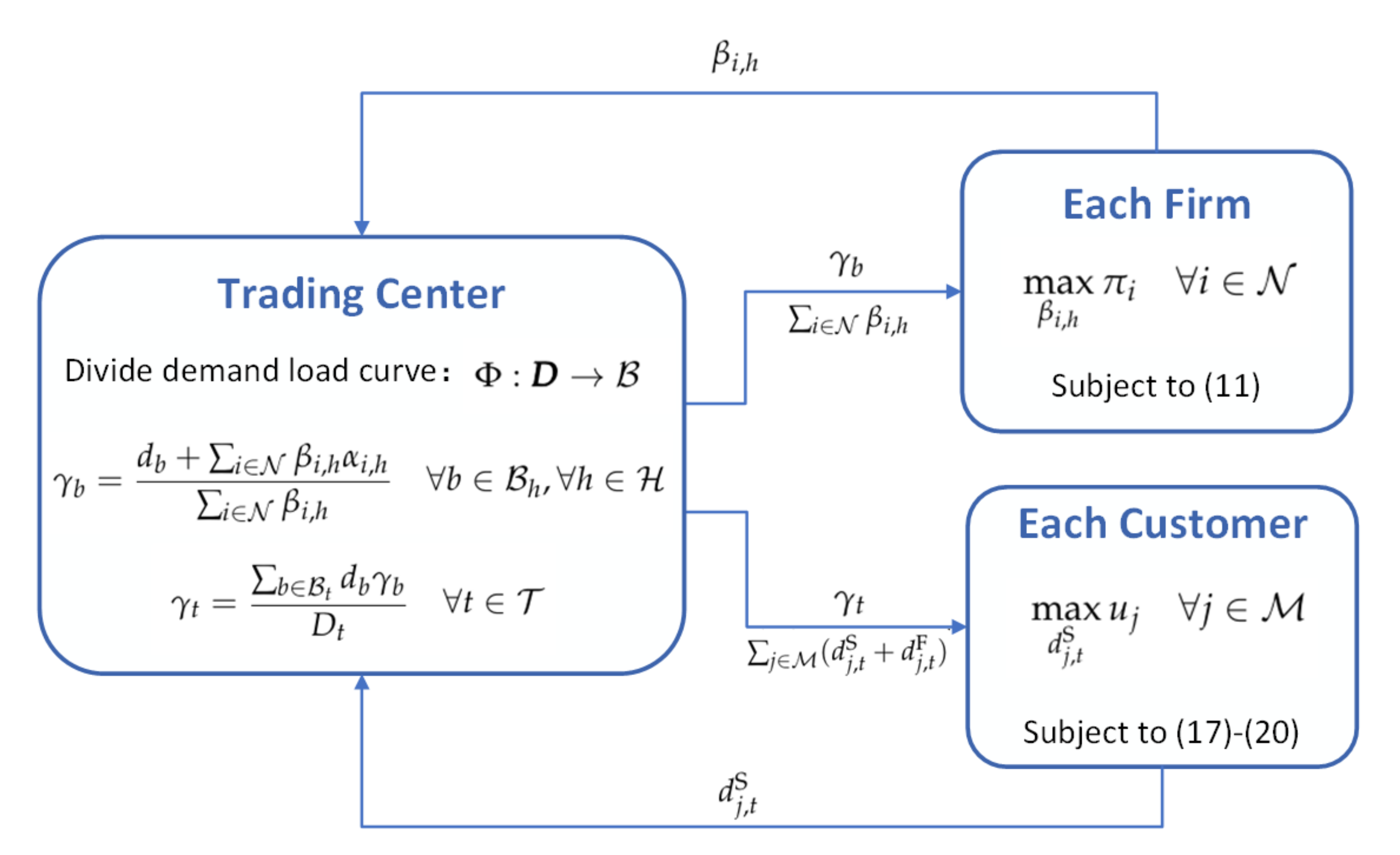
The interaction diagram of the trading center, each firm, and each customer can be shown in Figure 5.

We propose a distributed iterative approach for solving the double-sided non-cooperative game. The method will converge to the Nash equilibrium of supply-side and demand-side. We explain why the optimization problem of each firm and each customer can eventually converge to Nash equilibrium in the Appendix A.

For each firm, iteration can be achieved by the gradient ascent method. It is on the contrary to the gradient descent, which is a first-order iterative optimization algorithm for obtaining the local maximum of a function [21]. By deriving ${\pi }_i$ with respect to ${\beta }_{i,h}$, we can obtain:

$$\frac{\partial {\pi }_i}{\partial {\beta }_{i,h}}=\sum _{b\in {\mathcal{B}}_h}\left\{\frac{({\gamma }_b-{\alpha }_{i,h})({\sum }_{i\in \mathcal{N}}{\beta }_{i,h}-{\beta }_{i,h})}{{\sum }_{i\in \mathcal{N}}{\beta }_{i,h}}·\left[\frac{({\gamma }_b-{\alpha }_{i,h}){\beta }_{i,h}h}{{\sum }_{i\in \mathcal{N}}{\beta }_{i,h}-{\beta }_{i,h}}+{\gamma }_{b}h-\frac{\partial C_{i,b}}{\partial q_{i,b}}\right]\right\}\forall h\in \mathcal{H},\forall i\in \mathcal{N}$$

(25)

where

$$\frac{\partial C_{i,b}}{\partial q_{i,b}}=(c_{i,h}{q}_{i,b}+a_{i,h})h\forall b\in {\mathcal{B}}_h,\forall h\in \mathcal{H},\forall i\in \mathcal{N}$$

(26)

Subsequently, the iterative expression can be described as:

$${\beta }_{i,h}(m+1)={\beta }_{i,h}\left(m\right)+{\eta }_1\frac{\partial {\pi }_i\left(m\right)}{\partial {\beta }_{i,h}\left(m\right)}\forall h\in \mathcal{H},\forall i\in \mathcal{N}$$

(27)

where m denotes the iteration number and ${\eta }_1$ is the step size.

For the demand-side game, the gradient can not be directly calculated due to the nonlinear mapping from the demand load curve to the divided load blocks in (17). Therefore, the gradient is estimated by the finite forward difference. We apply the active set algorithm [22] to solve the demand-side game model and [23,24] demonstrate how the algorithm converges to a local optimal solution that satisfies the constraints. The algorithm finds active constraints on decision variables in each generation, and establishes a direction of search at each iteration by processing the finite-difference. The iterative expression can be described as:

$$d_{j,t}^{\mathrm{S}}(m+1)=d_{j,t}^{\mathrm{S}}\left(m\right)+{\left[{\eta }_2·F{D}_j\right]}^{\mathrm{A}}\forall t\in \mathcal{T},\forall j\in \mathcal{M}$$

(28)

where ${\eta }_2$ denote the iterative step size of the demand-side game, $F{D}_j$ denote the forward difference of customer j, and ${[·]}^{\mathrm{A}}$ means to handle the finite-difference through the active set algorithm.

The block division method in (1) and (2) for the trading center in block bidding markets can refer to the Load Division Method in [16]. This method is based on the principle of bottom-up, and the load blocks are divided in order from a long duration to short. It can be noted that, for each firm, the block-based price ${\gamma }_b$ and the sum of firms’ bids ${\sum }_{i\in \mathcal{N}}{\beta }_{i,h}$ should be informed by the trading center. For each customer, we assume the same block division method is applied in (17). The trading center should inform the time-based price ${\gamma }_t$ and the sum of customers’ demands ${\sum }_{j\in \mathcal{M}}(d_{j,t}^{\mathrm{S}}+d_{j,t}^{\mathrm{F}})$ in each iteration. The other necessary variables, such as ${\sum }_{i\in \mathcal{N}}{\beta }_{i,h_b}{\alpha }_{i,h_b}$ and ${\sum }_{i\in \mathcal{N}}{\beta }_{i,h_b}$ in (16), can be calculated by (3) and (8).

The overall distributed iterative algorithm is described in Algorithm 1, where $\epsilon$ denotes the convergence accuracy.

Algorithm 1 Distributed iterative algorithm of the double-sided non-cooperative game.

Require:  The initial demand load curve $\mathit{D}\left(0\right)$; The initial strategic variables ${\beta }_{i,h}\left(0\right)$ and $d_{j,t}^{\mathrm{S}}\left(0\right)$;

Parameters of the profit function (9) and the payoff function (15);

Ensure:  The optimal strategy for each firm and each customer; the block-based and time-based

electricity prices.

1: Initialize $m=0$, $\epsilon ={10}^{-3}$

2: repeat

3:   The trading center informs ${\gamma }_b\left(m\right)$ and ${\sum }_{i\in \mathcal{N}}{\beta }_{i,h}\left(m\right)$ to each firm, and informs ${\gamma }_t\left(m\right)$ and

${\sum }_{j\in \mathcal{M}}(d_{j,t}^{\mathrm{S}}\left(m\right)+d_{j,t}^{\mathrm{F}})$ to each customer;

4:   for each firm i from 1 to N do

5:    ${\displaystyle {\beta }_{i,h}(m+1)={\beta }_{i,h}\left(m\right)+{\eta }_1\frac{\partial {\pi }_i\left(m\right)}{\partial {\beta }_{i,h}\left(m\right)}}$;

6:   end for

7:   for each customer j from 1 to M do

8:    $d_{j,t}^{\mathrm{S}}(m+1)=d_{j,t}^{\mathrm{S}}\left(m\right)+{\left[{\eta }_2·F{D}_j\right]}^{\mathrm{A}}$;

9:   end for

10:   The trading center calculates $D_t(m+1)$ by (12)-(13); divides load blocks and obtains $\mathcal{B}(m+1)$,

$d_b(m+1)$ and $h_b(m+1)$; calculates ${\gamma }_b(m+1)$ by (8); calculates ${\gamma }_t(m+1)$ by (3);

11:   $m=m+1$;

12: until$|{\beta }_{i,h}\left(m\right)-{\beta }_{i,h}(m-1)|<\epsilon$, $|d_j^{\mathrm{S}}\left(m\right)-d_j^{\mathrm{S}}(m-1)|<\epsilon$, $|{\gamma }_t\left(m\right)-{\gamma }_t(m-1)|<\epsilon$

13: Each customer solves the shiftable loads’ positioning problem (21)-(24) to obtain $x_{j,k,t}^{*}$;

14: return the optimal solution ${\beta }_{i,h}^{*}$, $x_{j,k,t}^{*}$, and the electricity price ${\gamma }_t^{*}$, ${\gamma }_b^{*}$;

4. Simulation and Analysis

In this section, we demonstrate the effectiveness of the proposed model and algorithm through two simulations. Firstly, we simulate a system of three firms and 10 customers to show the effectiveness of the proposed model on peak shaving, expenditure reducing, costs reducing, and welfare improving. Secondly, we analyze the convergence process of Algorithm 1 and simulate the algorithm for different number of firms and customers to show the applicability of the algorithm on large systems.

In the simulation of the double-sided non-cooperative game in block bidding markets, we divide a trading day into 24 time-slots, and each time-slot represents an hour. As illustrated in Section 2.2, the positive coefficients $c_{i,h}$ and $a_{i,h}$ of cost functions for each firm are smaller when the block duration h is longer.

Table 1. Ranges of coefficients in firms’ cost functions.

Duration of Load Blocks (h)	Quadratic Coefficients $\left({\mathit{c}}_{\mathit{i},\mathit{h}}\right)$	Linear Coefficients $\left({\mathit{a}}_{\mathit{i},\mathit{h}}\right)$
1–3	[8, 8.1]	[1.1, 1.2]
4–7	[7.4, 7.5]	[0.9, 1.0]
8–11	[6.8, 6.9]	[0.7, 0.8]
12–23	[6.1, 6.2]	[0.38, 0.40]
24	[0.18, 0.2]	[0.08, 0.09]

defines the ranges of $c_{i,h}$ and $a_{i,h}$. The coefficients ${\omega }_{j,t}$ of customers’ satisfaction functions is randomly selected in range [10, 13], and $v_{j,t}$ is set to 0.5. The supply-side step size ${\eta }_1$ is set to 0.001. The demand-side finite-difference step size $\delta$ is set to 0.2, and the iterative step size ${\eta }_2$ is dynamically set by the active set algorithm. The convergence accuracy $\epsilon$ is set to ${10}^{-3}$. The pre-chosen values of ${\alpha }_{i,h}$ are set to the intercept $a_{i,h}$ of the marginal cost.

Customers’ demand load data are generated from real data in [25]. Shiftable load resources are collected from [26] and listed in

Table 2. Information of Shiftable Loads [26].

Appliance Type	Power Demand (kW)	Deman Duration (h)
vacuum cleaner	1.2	1
electric vehicle	3.5	3
dish washer	1.0	3
washing machine	1.0	2
dryer	3.0	1
laptop	0.1	2

. The daily fixed load demands for each customer is about 67 kW·h to 124 kW·h. For each customer, there are about 4–10 shiftable loads, the power demands of shiftable loads are about 15–20% of their daily total demands. Without a loss of generality, shiftable loads’ time frame $\left[t_{j,\kappa }^{min},t_{j,\kappa }^{max}\right]$ are set to [1, 24]. Simulation is realized on MATLAB platform. Demand-side active-set algorithm is executed by fmincon [27], and positioning problem (21)–(24) is solved by Yalmip [28] and Cplex [29]. The data of fixed loads and shiftable loads and the programs of this system are attached in [30].

4.1. Case Study

In this subsection, we simulate and analyze two cases. Without DR case is the solution without customers’ DR, but only firms’ optimal bidding. With DR case is the optimal solution of Algorithm 1.

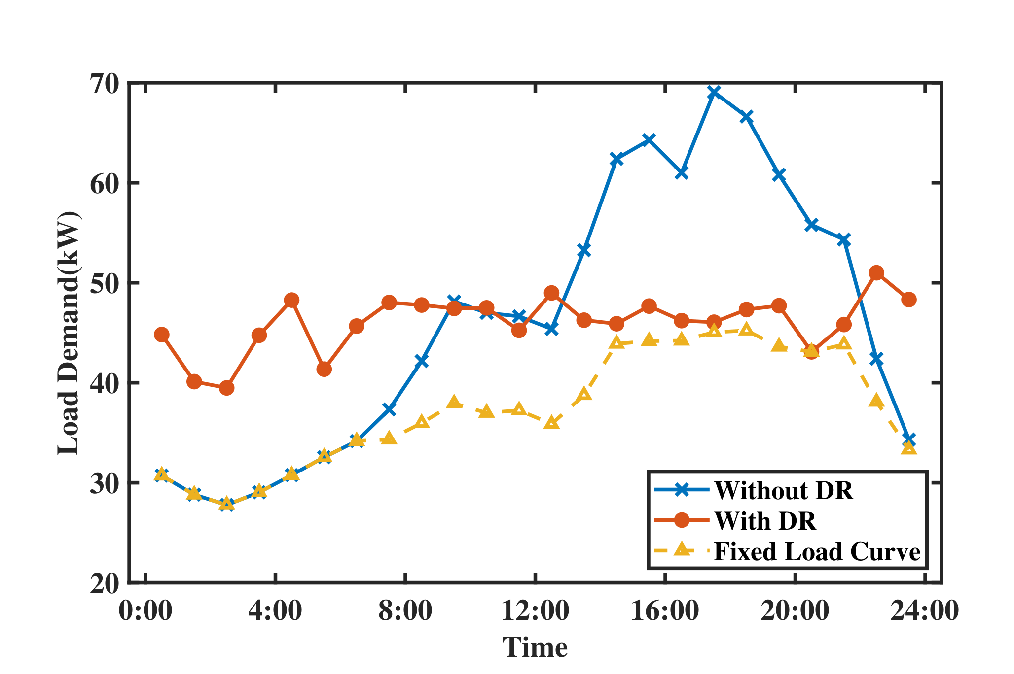
Figure 6 shows the aggregate fixed and total demand load curves with and without DR. From the aggregate load curve during 14:00–22:00, we can notice that the proposed model with DR can greatly achieve peak shaving. The peak load without DR is 69.05 kW, and decreases to 50.99 kW with DR. Many loads at peak hours are moved to valley periods by customers, and the overall load curve is significantly flattened. The 24-h load power without DR is 27.78 kW, and becomes to 39.48 kW with DR. Moreover, in time-slots with similar prices, shiftable loads for each customer are shifted to time-slots with higher ${\omega }_{j,t}$.

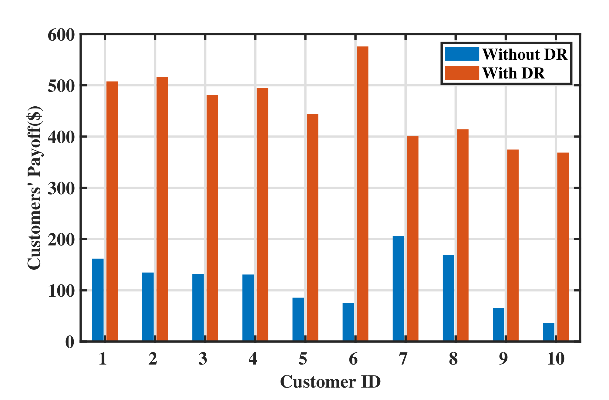
Figure 7 show the daily payoff for customers 1–10 with and without the DR program. By participating in DR, customers’ payoff increases a lot. The daily payoff of each customer with DR is around 4.77 times of its value without DR. Customers’ different payoff are due to their different satisfaction functions.

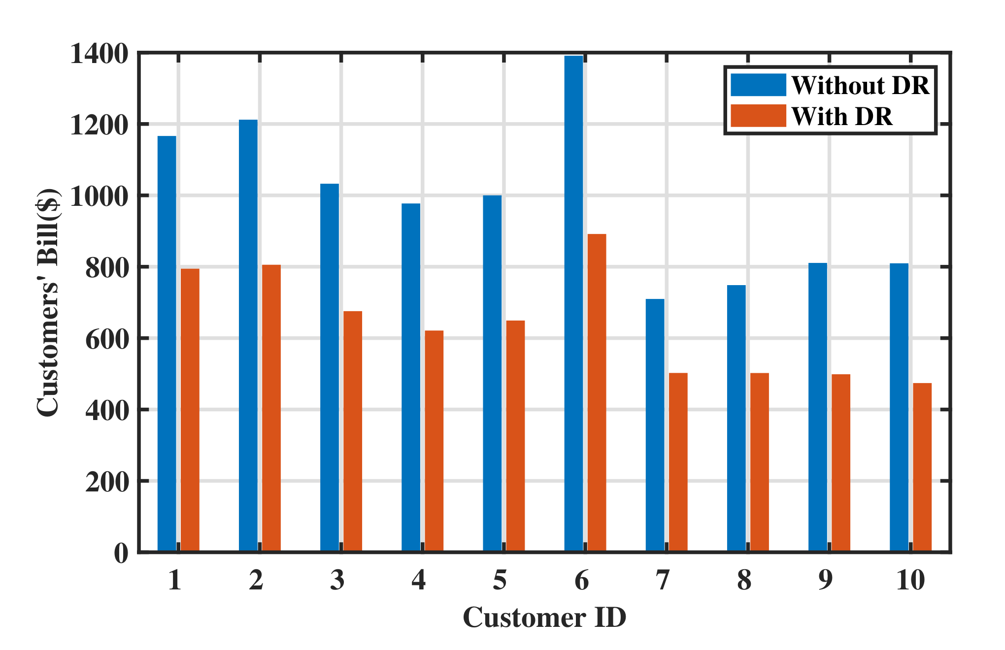
Moreover, the daily bill of customers decreases with DR. Figure 8 shows the bill of customers 1–10. Each customer’s daily bill with DR is around 65% of its value without DR. In other words, customers can save approximately 35% of electricity expenses by participating in DR.

In the supply-side game, Figure 9 shows firms’ daily costs. With the DR program, the costs of each firm can obtain an average decrease of about 35.24%. This is because the total load curve becomes flatter, and the 24-h load capacity increases a lot. Longer duration load blocks can help to reduce start–stop expenses and obtain lower generation costs. Meanwhile, by the optimal bidding of power firms, their daily revenue is also maximized.

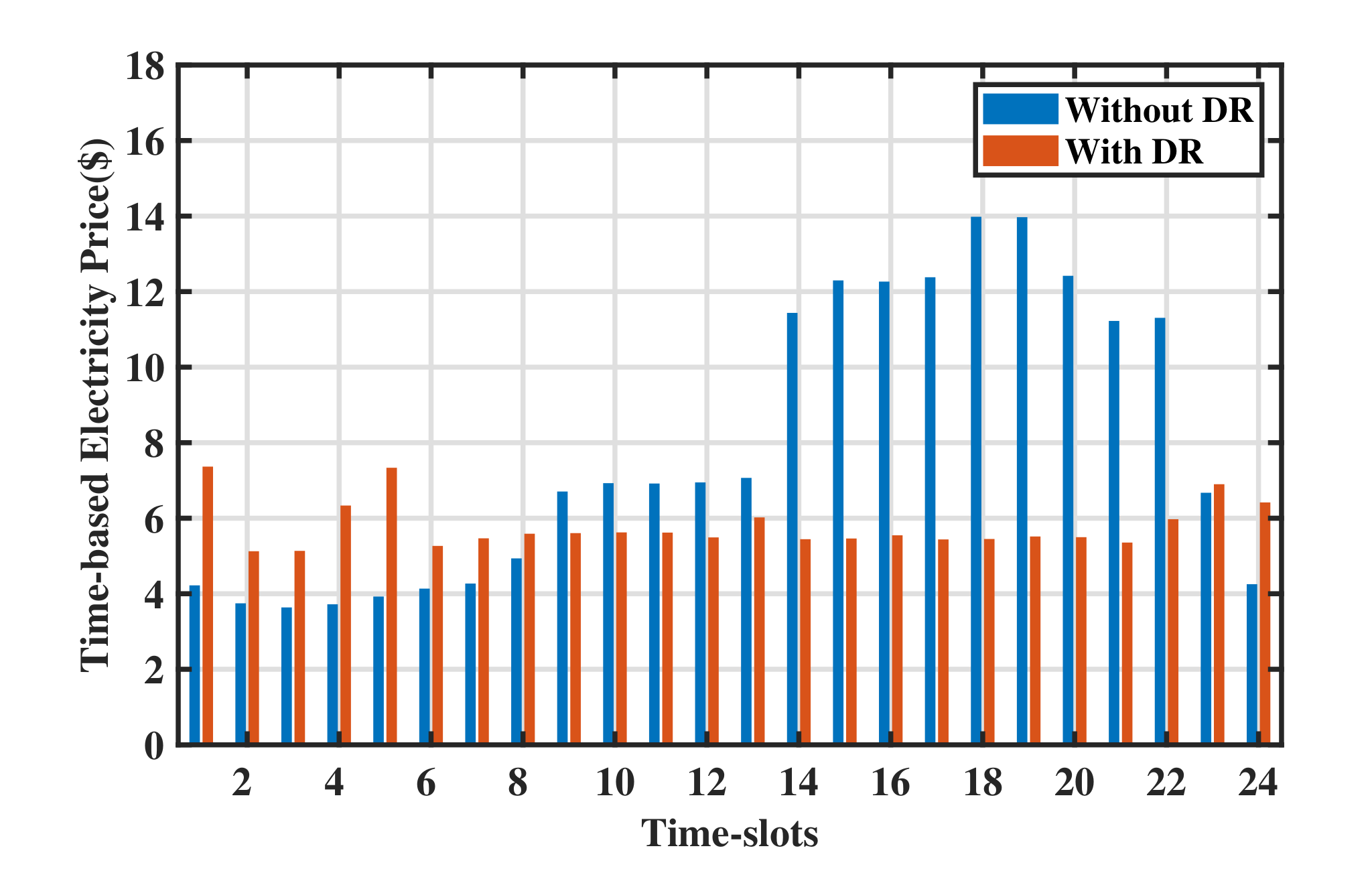
Figure 10 shows the market time-based electricity price. It can be seen that the overall trend of electricity prices is similar to the aggregate load curve shown in Figure 6. The daily electricity prices become flatten with DR, and the price variance decreases from 14.1708 to 0.4012. Furthermore, the average price without DR is 7.8906 $/(kW·h) and it decreases to 5.7913 $/(kW·h) with the DR program. Therefore, the proposed model has a positive significance for reducing the market electricity prices.

We assess the market performance with and without DR by comparing total customer expenditure, generation costs, and social welfare. The results are listed in

Table 3. Comparison of market performance with and without DR.

Cases	Total Customer Expenditure ($)	Total Generation Costs ($)	Social Welfare ($)
Without DR	9858.10	2699.11	8354.12
With DR	6415.27	1747.82	9244.43

, where social welfare is calculated by the following equation:

$$SW=\sum _{j\in \mathcal{M}}\sum _{t\in \mathcal{T}}{W}_{j,t}\left(d_{j,t}^{\mathrm{F}}+d_{j,t}^{\mathrm{S}}\right)-\sum _{i\in \mathcal{N}}\sum _{h\in \mathcal{H}}\sum _{b\in {\mathcal{B}}_h}{C}_{i,b}\left(q_{i,b}\right)$$

(29)

According to Table 3, customers’ participation of DR can improve the social welfare, while greatly reducing the electricity expenditure and generation costs. Although the maximization of social welfare is not considered in the mathematical model, the results show the positive effect of the proposed model on society. This is a win–win situation for all parties. Each firm and each customer only care about their own utility, but brings about a 10% increase in social welfare.

4.2. Convergence Characteristics and Model Scale

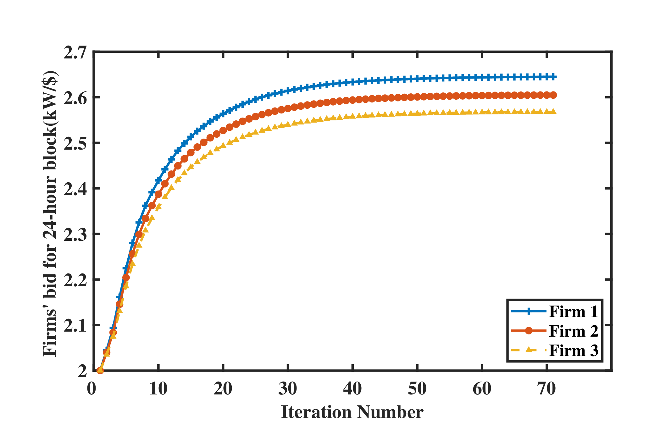
The convergence ability of an algorithm is a key factor for measuring its performance, and determines whether the model can be applied to a larger system. Therefore, we analyze the convergence characteristics of Algorithm 1 in this subsection. Figure 11 shows the convergence process of firms’ bids on the 24-h load block. It can be seen that the bids start from the same initial values and converge to the Nash equilibrium. Firms have different optimal bids, because they have different generation cost functions. The algorithm converges in 71 iterations with about 77 s. The convergence time is closely related to the step size setting.

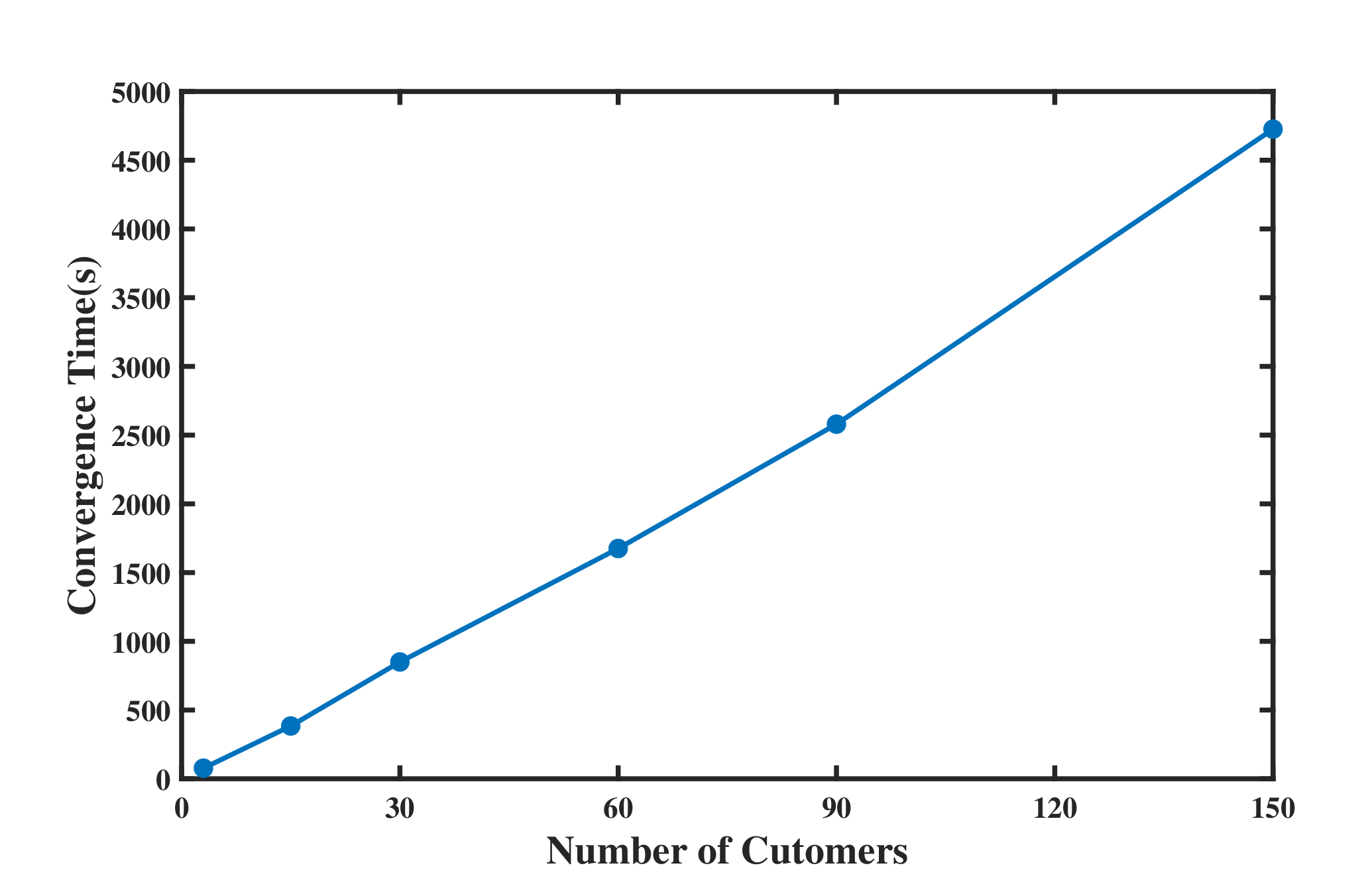
In order to better reflect the computational complexity of the proposed algorithm, we simulate the algorithm for different number of firms and customers, and present the relationship between the convergence time and the system scale in Figure 12. It can be seen that, as the number of customers increases, the solution time increases linearly. For a system of 150 customers, the solution time is within 5000 s. Each firm and each customer should optimize their own strategy, but we use FOR-loop to solve the distributed algorithm in simulation, as expressed in Algorithm 1. Therefore, the actual distributed solution time will be much shorter than the results that are shown in Figure 12.

4.3. Energy Policy Discussion

In the Nash equilibrium of the double-sided non-cooperative game, each firm obtains the optimal slope ${\beta }_{i,h}$ of supply curve for each block duration, which corresponds to the power supply $q_{i,b}$ for each block.

Table 4. Part of the obtained optimal strategy of Firm 1.

Block ID	Power Supply (kW)	Running Duration (h)	Running Time-Slots	Unit Price ($)
1	13.3622	24	1–24	5.2916
2	0.6250	21	4–24	7.3216
3	0.7161	14	7–20	10.7481
4	0.1411	5	7–11	10.0982
5	1.1299	2	4–5	13.4156
6	1.5689	1	1	12.5358

shows part of the obtained optimal operation strategy of Firm 1.

It can be noted from Table 4 that the power supply, running duration, running time-slots, and electricity prices are all settled down by the Nash equilibrium. Therefore, firms do not need to solve further optimization problems in order to obtain the operating strategy for generation units. Instead, they can easily arrange units’ operation, for example, let a unit running from one to 24 time-slots at 13.3622 kW. In addition, the price is closely related to the power generation cost of each block, so it can well reflect the core idea of “the same quality, the same price”.

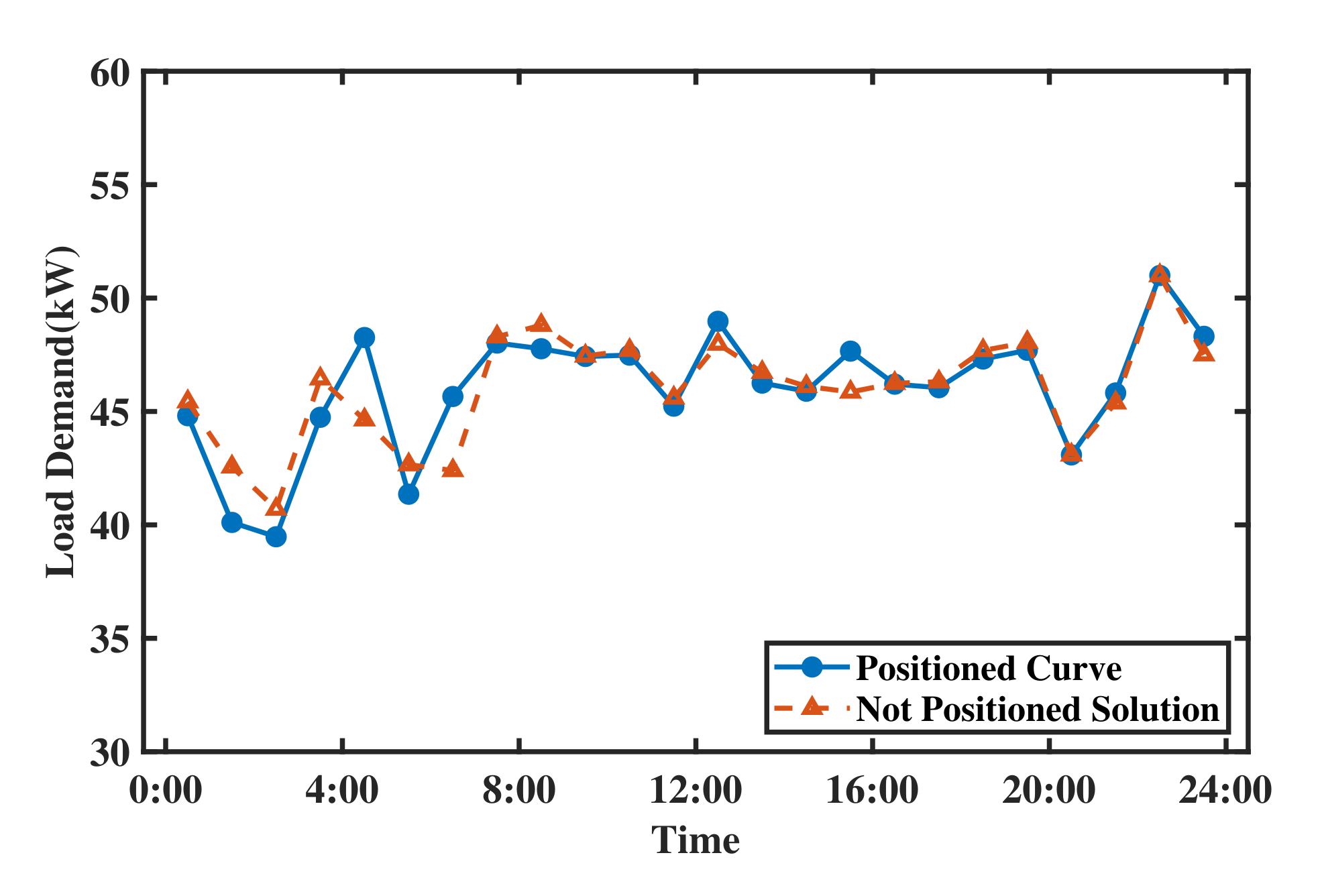
After obtaining the Nash equilibrium solution, each customer in the non-cooperative game solves the shiftable loads’ positioning problem (21)–(24) to obtain the exact operating time-slots of shiftable loads. Figure 13 shows the positioning results of shiftable loads.

From Figure 13, it can be noted that the positioned curve will not deviate much from the Nash equilibrium solution, and the error is within the allowable range. By executing the payoff maximization problem and the positioning problem, each customer can obtain their own strategy.

Table 5. Part of the obtained optimal strategy of Customer 1.

Shiftable Load ID	Appliance Type	Power Demand (kW)	Duration (h)	Running Time-Slots
1	electric vehicle	3.5	3	2, 5, 24
2	washing machine	1	2	2, 24
3	vacuum cleaner	1.2	1	2
4	dish washer	1	3	2, 12, 24
5	dryer	3	1	24
6	dish washer	1	3	2, 11, 24

shows part of the obtained optimal strategy of Customer 1.

As can be seen, each shiftable load of this customer is arranged with specific running time-slots, satisfying the running duration constraints. Most shiftable loads are scheduled to time-slot 2 and 24. This is because the power of fixed loads during these two time-slots are lower, and the satisfaction coefficient ${\omega }_{j,t}$ is relatively higher. However, letting each customer manually execute the decision according to the table is not easy. Therefore, the strategy puts a high demand on smart meters and smart homes. With the popularity of intelligent household appliances, customers can easily obtain the maximum payoff while getting rid of switching appliances.

5. Conclusions

This paper studies the non-cooperative game behavior of multiple firms and multiple customers in competitive block bidding markets. Under the block market rules, the demand load should be divided into continuous blocks and traded at block prices. We propose a distributed market architecture, and the trading center is responsible for converting block-based prices to hourly-various prices. The supply-side game is based on supply function bidding for each block, and it realizes each firm’s profit maximization. The demand-side game considers fixed loads and shiftable loads, and it achieves each customer’s payoff maximization. The positioning model for each customer is used to determine the actual operating time-slots of shiftable loads. We propose a distributed iterative algorithm that is based on gradient ascent and active set to solve the double-sided optimization problem. The proposed model is applied on an actual case and is simulated based on real data. Simulation results show that the proposed model with DR can greatly achieve peak shaving, and the overall load curve is flattened. Customers’ electricity expenditure and firms’ generation costs both reduce a lot, and the social welfare is significantly improved meanwhile. Besides, the model has a positive significance for reducing the market prices. The distributed algorithm can converge to Nash equilibrium in large systems within acceptable iteration and time. In the Nash equilibrium, each firm can easily arrange units’ operation without solving further optimization problems, and each customer can obtain the specific running time-slots of shiftable loads.

In the future, we will model both block bids and hourly bids in electricity markets. In addition, we will compare the effects of the two mechanisms on peak shaving, energy cost-reducing, and social welfare improving with real scenarios and data.

References

1. Sun, J.; Ruze, N.; Zhang, J.; Zhao, H.; Shen, B. Evaluating the Investment Efficiency of China’s Provincial Power Grid Enterprises under New Electricity Market Reform: Empirical Evidence Based on Three-Stage DEA Model. Energies 2019, 12, 3524. [Google Scholar] [CrossRef] [Green Version]
2. Dawn, S.; Tiwari, P.K.; Goswami, A.K. An approach for long term economic operations of competitive power market by optimal combined scheduling of wind turbines and FACTS controllers. Energy 2019, 181, 709–723. [Google Scholar] [CrossRef]
3. Wang, T.; Zhang, D.; Ji, Q.; Shi, X. Market reforms and determinants of import natural gas prices in China. Energy 2020, 196, 117105. [Google Scholar] [CrossRef]
4. Wang, X.; Guan, X.; Wang, X. Block bidding power markets. In Proceedings of the International Conference on Power System Technology, Kunming, China, 13–17 October 2002; Volume 3, pp. 1828–1832. [Google Scholar]
5. Nord Pool: Block Order. Available online: https://www.nordpoolgroup.com/trading/Day-ahead-trading/Order-types/Block-bid/ (accessed on 26 May 2020).
6. Lezama, F.; Faia, R.; Faria, P.; Vale, Z. Demand Response of Residential Houses Equipped with PV-Battery Systems: An Application Study Using Evolutionary Algorithms. Energies 2020, 13, 2466. [Google Scholar] [CrossRef]
7. Park, H. Human Comfort-Based-Home Energy Management for Demand Response Participation. Energies 2020, 13, 2463. [Google Scholar] [CrossRef]
8. Abrishambaf, O.; Faria, P.; Vale, Z. Ramping of Demand Response Event with Deploying Distinct Programs by an Aggregator. Energies 2020, 13, 1389. [Google Scholar] [CrossRef] [Green Version]
9. Nash, J. Non-cooperative games. Ann. Math. 1951, 286–295. [Google Scholar] [CrossRef]
10. Shah, D.; Chatterjee, S. Optimal Placement of Time Flexible Supplier’s Block Bid in a Day-Ahead Electric Market using Genetic Algorithm. In Proceedings of the 2019 Second International Conference on Advanced Computational and Communication Paradigms (ICACCP), Sikkim, India, 25–28 February 2019; pp. 1–8. [Google Scholar]
11. Zak, E.J.; Ammari, S.; Cheung, K.W. Modeling price-based decisions in advanced electricity markets. In Proceedings of the 2012 9th International Conference on the European Energy Market, Florence, Italy, 10–12 May 2012; pp. 1–6. [Google Scholar]
12. Bhardwaj, A.; Saxena, A. Optimal Bidding Strategy for Profit Maximization of Generation Companies under Step-Wise Bidding Protocol. Int. J. Eng. Technol. 2017, 9, 797–805. [Google Scholar] [CrossRef] [Green Version]
13. Kamyab, F.; Amini, M.; Sheykhha, S.; Hasanpour, M.; Jalali, M.M. Demand response program in smart grid using supply function bidding mechanism. IEEE Trans. Smart Grid 2015, 7, 1277–1284. [Google Scholar] [CrossRef]
14. Chai, B.; Chen, J.; Yang, Z.; Zhang, Y. Demand Response Management With Multiple Utility Companies: A Two-Level Game Approach. IEEE Trans. Smart Grid 2014, 5, 722–731. [Google Scholar] [CrossRef]
15. Elghitani, F.; Zhuang, W. Aggregating a Large Number of Residential Appliances for Demand Response Applications. IEEE Trans. Smart Grid 2018, 9, 5092–5100. [Google Scholar] [CrossRef]
16. Guo, N.; Wang, Y.; Xu, Z.; Yan, G. Optimal pricing strategy of power-retailing companies considering demand response in block bidding markets. IET Gener. Transm. Distrib. 2020, 14, 1641–1652. [Google Scholar] [CrossRef]
17. Sanchez de la Nieta, A.A.; Gibescu, M. Maximal Daily Social Welfare Through Demand Side Management in the Day-Ahead Electricity Market. In Proceedings of the 2018 15th International Conference on the European Energy Market (EEM), Lodz, Poland, 27–29 June 2018; pp. 1–5. [Google Scholar]
18. Motalleb, M.; Ghorbani, R. A Game Theoretic Model of Demand Response Aggregator Competition for Selling Stored Energy in Regulated and Unregulated Power Markets. arXiv 2016, arXiv:1612.00716. [Google Scholar]
19. Khanna, S.; Becerra, V.; Allahham, A.; Giaouris, D.; Foster, J.M.; Roberts, K.; Hutchinson, D.; Fawcett, J. Demand Response Model Development for Smart Households Using Time of Use Tariffs and Optimal Control—The Isle of Wight Energy Autonomous Community Case Study. Energies 2020, 13, 541. [Google Scholar] [CrossRef] [Green Version]
20. Baldick, R. Electricity market equilibrium models: The effect of parametrization. IEEE Trans. Power Syst. 2002, 17, 1170–1176. [Google Scholar] [CrossRef] [Green Version]
21. Ruder, S. An overview of gradient descent optimization algorithms. arXiv 2016, arXiv:1609.04747. [Google Scholar]
22. Ferreau, H.J.; Kirches, C.; Potschka, A.; Bock, H.; Diehl, M. qpOASES: A parametric active-set algorithm for quadratic programming. Math. Program. Comput. 2014, 6, 327–363. [Google Scholar] [CrossRef]
23. Powell, M.J.D. A fast algorithm for nonlinearly constrained optimization calculations. In Numerical Analysis; Watson, G.A., Ed.; Springer: Berlin/Heidelberg, Germany, 1978; pp. 144–157. [Google Scholar]
24. Powell, M.J.D. The convergence of variable metric methods for nonlinearly constrained optimization calculations. Nonlinear Program. 1978, 3, 27–63. [Google Scholar]
25. Muratori, M. Impact of Uncoordinated Plug-In Electric Vehicle Charging on Residential Power Demand-Supplementary Data; Technical Report; National Renewable Energy Laboratory: Washington, DC, USA, 2017. [Google Scholar] [CrossRef]
26. Woodbank Communications Ltd. Electropaedia: Battery and Energy Technologies—Electricity Demand. Available online: https://www.mpoweruk.com/electricity_demand.htm (accessed on 20 May 2020).
27. Mathworks. Fmincon: Find Minimum of Constrained Nonlinear Multivariable Function. Available online: https://ww2.mathworks.cn/help/optim/ug/fmincon.html (accessed on 20 May 2020).
28. Lofberg, J. YALMIP: A toolbox for modeling and optimization in MATLAB. In Proceedings of the 2004 IEEE International Conference on Robotics and Automation (IEEE Cat. No. 04CH37508), New Orleans, LA, USA, 2–4 September 2004; pp. 284–289. [Google Scholar]
29. IBM. IBM ILOG CPLEX Optimization Studio: CPLEX User’s Manual; IBM: Armonk, NY, USA, 1987. [Google Scholar]
30. Guo, N. Data for: Non-Cooperative Game in Block Bidding Markets Considering Demand Response, Mendeley Data v1 ed.; Elsevier: Amsterdam, The Netherlands, 2020. [Google Scholar] [CrossRef]
Figure 1. Hourly bidding mode and block bidding mode.
Energies 13 03322 g001
Figure 2. Architecture of double-sided game with N firms and M customers.
Energies 13 03322 g002
Figure 3. Schematic diagram of block division in block bidding markets.
Energies 13 03322 g003
Figure 4. A typical example of shiftable loads scheduling.
Energies 13 03322 g004
Figure 5. Block diagram of the proposed mathematical model.
Energies 13 03322 g005
Figure 6. Fixed and total load curve with and without demand response (DR).
Energies 13 03322 g006
Figure 7. Customers’ daily payoff with and without DR.
Energies 13 03322 g007
Figure 8. Customers’ daily bill with and without DR.
Energies 13 03322 g008
Figure 9. Firms’ daily costs with and without DR.
Energies 13 03322 g009
Figure 10. Time-based electricity price with and without DR.
Energies 13 03322 g010
Figure 11. Convergence process of firms’ strategic bids for the 24-h load block.
Energies 13 03322 g011
Figure 12. Convergence time of Algorithm 1 with different number of customers.
Energies 13 03322 g012
Figure 13. Demand load curve before/after positioning shiftable loads’ operating time-slots.
Energies 13 03322 g013