Article

SimBench—A Benchmark Dataset of Electric Power Systems to Compare Innovative Solutions Based on Power Flow Analysis

1
Department of Energy Management and Power System Operation (e2n), University Kassel, 34121 Kassel, Germany
2
Institute for Energy Systems, Energy Efficiency and Energy Economy (ie3), TU Dortmund University, 44227 Dortmund, Germany
3
Fraunhofer Institute for Energy Economics and Energy System Technology (IEE), 34119 Kassel, Germany
4
Institute of Power Systems and Power Economics (IAEW), RWTH Aachen University, 52062 Aachen, Germany
*
Author to whom correspondence should be addressed.
Energies 2020, 13(12), 3290; https://doi.org/10.3390/en13123290
Submission received: 15 May 2020 / Revised: 10 June 2020 / Accepted: 22 June 2020 / Published: 26 June 2020

Abstract

:
Publicly accessible, elaborated grid datasets, i.e., benchmark grids, are well suited to publish and compare methods or study results. Similarly, developing innovative tools and algorithms in the fields of grid planning and grid operation is based on grid datasets. Therefore, a general methodology to generate benchmark datasets and its voltage level dependent implementation is described in this paper. As a result, SimBench, a comprehensive dataset for the low, medium, high and extra-high voltage level, is presented. Besides grids that can be combined across several voltage levels, the dataset offers an added value by providing time series for a whole year as well as future scenarios. In this way, SimBench is applicable for many use cases and simplifies reproducing study results. As proof, different automated algorithms for grid planning are compared to show how to apply SimBench and make use of it as a simulation benchmark.

1. Introduction

Many studies are conducted to apply innovative, grid-related solutions and technologies in electrical power systems. Such studies are usually based on simulations with power flow analyses which require electric steady-state grid model data. Studies from scientific literature and data published on websites, such as [1,2], provide a number of different grid model datasets. Among the most popular of these datasets are, for example, the IEEE test cases [3] and the CIGRE benchmark systems [4]. The reviews in [5,6], also introduce many more grids, their properties and focuses, such as the European representative electricity distribution networks [7], the representative distribution networks of Italy named Atlantide [8,9,10], the IEEE reliability test system [11,12] or the PEGASE and RTE cases [13,14].

1.1. Motivation

Power systems shift to a more sustainable energy supply via new technologies and corresponding regulatory frameworks. First, this constant shift leads to a rising gap between existing publicly accessible grid data and real power systems. Second, studies considering new technologies, regulatory frameworks and innovative solutions may have altered requirements for grid data compared to studies several years ago. Therefore, new publicly accessible grid data is needed to address these issues.
In addition, for the operation of increasingly smart grids, investigating the collaborative operation of different voltage levels and system operators becomes more important. This is because the increasing number of renewable energy sources is mainly connected to low voltage (LV), medium voltage (MV), and high voltage (HV) levels while the decreasing number of conventional power plants is mainly connected to extra-high voltage (EHV) and HV levels. To this date, publicly accessible grid data, which enable a combined modeling of voltage levels and feature sufficient detail and realistic scale, are rare. Therefore many publications, e.g., [15], use grid data of different origins which must be merged and harmonized. However, even if published studies use open grid data and perfectly describe the assumptions made and the applied calculation methods, it is often hard to reproduce the results and to compare the applied method with other ones. Frequent reasons for this are modifications to the investigated grids, conflicting assumptions and additional types of required data, such as load and generation time series. A solution would be a holistic dataset providing consistent data for all common German voltage levels. However, to the best of our knowledge, there is no dataset providing consistent data for all common German voltage levels (LV: 0.4 kV, MV: 10 / 20 kV, HV: 110 kV, EHV: 380 kV).
A variety of power flow-based use cases exist. To make methods for such use cases comparable, the same grid should be used. In fact, assumptions on operation, e.g., limits and setpoints, should also be the same unless the assumptions are part of the method. Often, however, grid datasets do not provide such information. Furthermore, there are no widespread datasets including grids with both a state without overloadings and a future state, which may become subject to overloading due to increased intermittent power generation. Such a dataset would allow studying use cases which require grid states without loading limit violations as well as analyzing use cases which require violations to solve.

1.2. Introducing SimBench

To close the afore-mentioned gaps, this paper introduces a new dataset of electric steady-state grid models, compiled within the research project SimBench. It is intended as a benchmark to test, publish and compare methods and algorithms for various use cases, as already used in e.g., [16,17,18,19]. The use cases include the fields of grid planning, operation and simulation [20,21]. SimBench data are published online [1] under Open Data Common Open Database Licence (ODbL, data are available at https://opendatacommons.org/licenses/odbl/1.0/ and https://simbench.de/en/downloads). While the SimBench dataset is based on power grids in Germany, this paper describes the methodology to compile the benchmark dataset, in order to enable the scientific community to compile compatible datasets for other regions. To facilitate its use in a variety of application contexts, the SimBench dataset is published in four different data formats. These include the format of the open-source power system analyzing and optimizing tool pandapower [22], formats of the commercial tools DIgSILENT PowerFactory [23] and INTEGRAL [24] and a format especially created for the SimBench data. This SimBench format is based on CSV file tables, which can also be evaluated by researchers directly using common spreadsheet applications [21].
This paper is organized as follows. In Section 2, the developed and applied methodology of SimBench is described. In Section 3, an overview of the data of the grids, the time series and the future scenarios is provided. In Section 4, a case study shows how SimBench data can be used to compare different algorithms. Finally, some conclusions are drawn in Section 5.

2. Methodology to Compile the SimBench Dataset

Within SimBench, a general methodology to compile benchmark grids has been developed [20], which makes it possible to compile benchmark grids of different voltage levels or scopes. The developed methodology consists of the following six steps:
  • a clear formulation of the objectives,
  • a comprehensive view of the task and a literature review,
  • a determination of use case requirements,
  • an analysis of available data,
  • the compilation of the grid dataset and
  • the evaluation of the dataset.
An iterative loop of Step 5 and 6 ensures appropriateness and applicability of the dataset. Since the methodology is described in reference [20], this paper gives only a brief overview of applying the methodology to create the SimBench dataset.

2.1. Voltage Level Dependent Methods to Generate the Grid Data

2.1.1. Extra-High and High Voltage Level

The methods used to generate the data for the EHV and the HV level were based on publicly accessible, geo-referenced data [25,26]. For the EHV level, a modification of the grid dataset from the SciGrid project is being developed [27]. Using algorithms developed within SimBench, coherent node-branch models were generated using SciGrid data. In addition, publicly accessible power plant data [28] and data on population densities from [29] as well as industrial loads are used to model the supply task. Based on the grid topology and the defined supply task, the grids were dimensioned for the N-1 state applying relevant use cases [30]. More details on the development of the SimBench HV grid and its origins in publicly accessible data are given in [31].

2.1.2. Medium Voltage Level

In comparison to the other voltage levels, the available open data for the MV level, such as data on building distribution as well as line and road maps or population information, have been found to be less significant, scarce or uncertain. Hence, as depicted in Section 3.3, the data analysis step for the MV grids is not to compile an extensive grid design, but to validate the SimBench grids against reality. In order to consider and balance the requirements of about 30 relevant use cases [21], as well as the information found in the literature review and the insights of analyzing the real grid data, the SimBench MV grids were generated manually.
A number of four MV grid classes were selected for the following reasons: On the one hand, this facilitates comparisons by restricting the complexity of the dataset. On the other hand, four grid classes can cover the essential and frequently occurring characteristics of existing grids. For example, in addition to the open ring topology occurring in all SimBench MV grids, a base station, a remote station and radial feeders were spread over the MV grids. As a result of this and of different busbar concepts, specific requirements were set for comparisons of methods, e.g., for checking (n−1)-security.

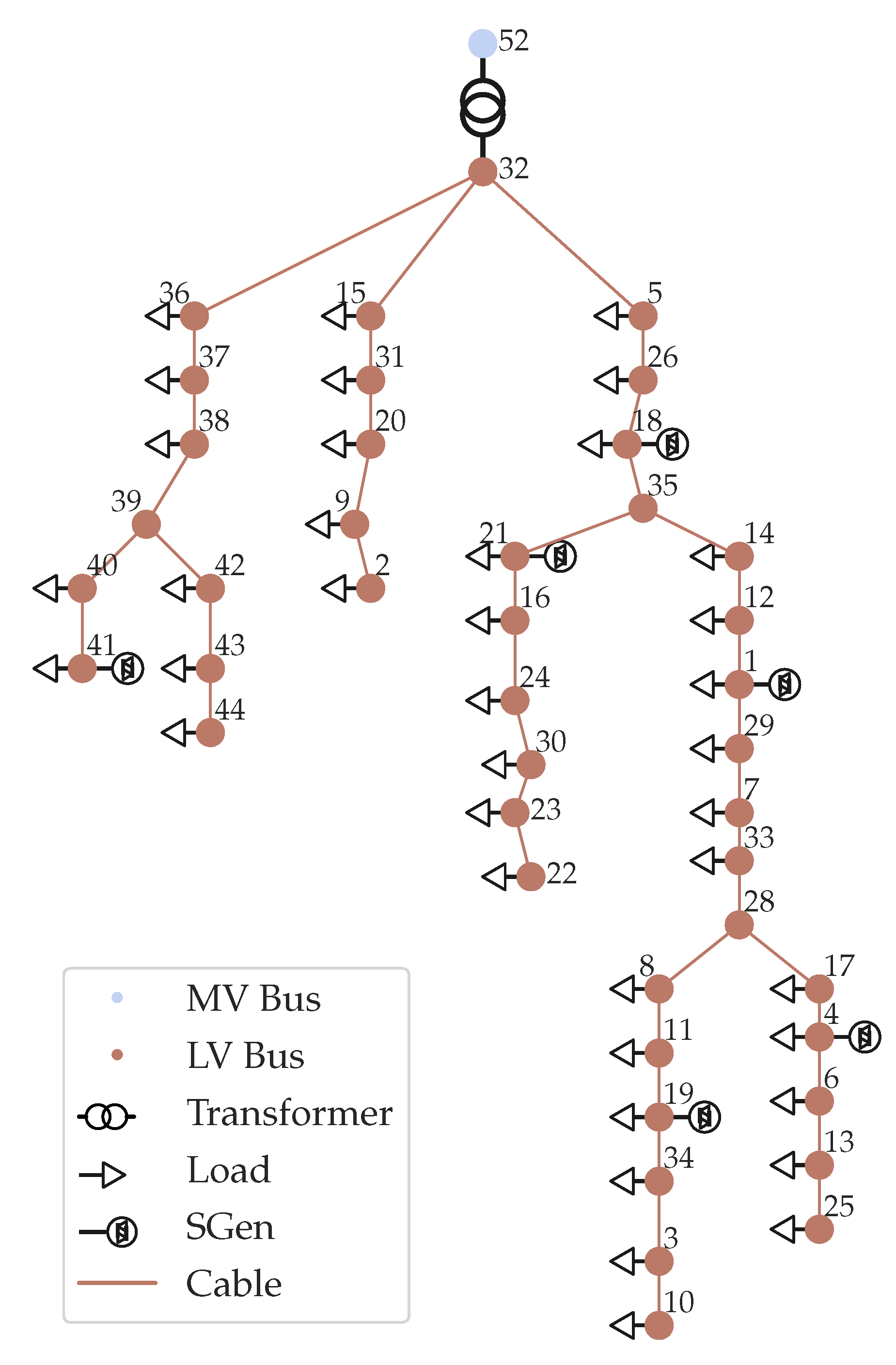
2.1.3. Low Voltage Level

The generation of the grids for the LV level includes two parts, the determination of the supply task and the automatic network model generation. The data required for this is derived from official statistics published by the German federal statistical office (DESTATIS) [29] and OpenStreetMap [25]. The supply task was classified using a k-means clustering algorithm. The detailed clustering results can be found in [32]. These results comprised six clusters, of which three are rural, two were semi-urban and one was urban. For the generation of the models, an automated algorithm was used, which is described in [33]. The algorithm provides a graph to ensure that the network models are initially available as node-edge models. Based on an evaluation of real data and with respect to the requirements, these were manually converted into an electrical grid model with load and generation units. The refined method for generating the SimBench LV grids is described in detail in [34].

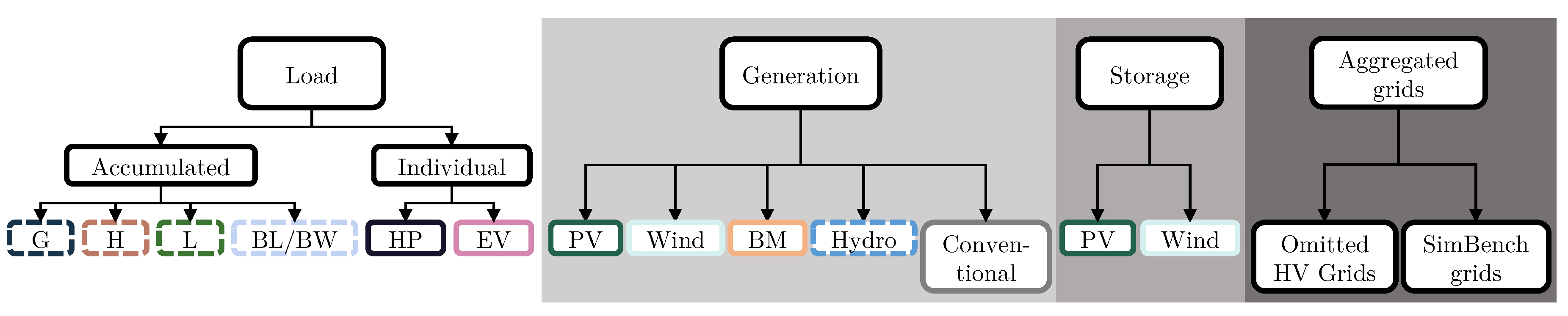
2.2. Approach for Compiling Time Series

SimBench includes multiple time series for one year with 15 min resolution for load, generation and storage units. All time series came as active and reactive power time series. The time series were normalized, reducing the total number of required time series to a reasonable number, while retaining the possibility to model individual nominal power. While a detailed explanations can be found in [35], this paper summarizes the applied time series methods with respect to the types displayed in Figure 1.

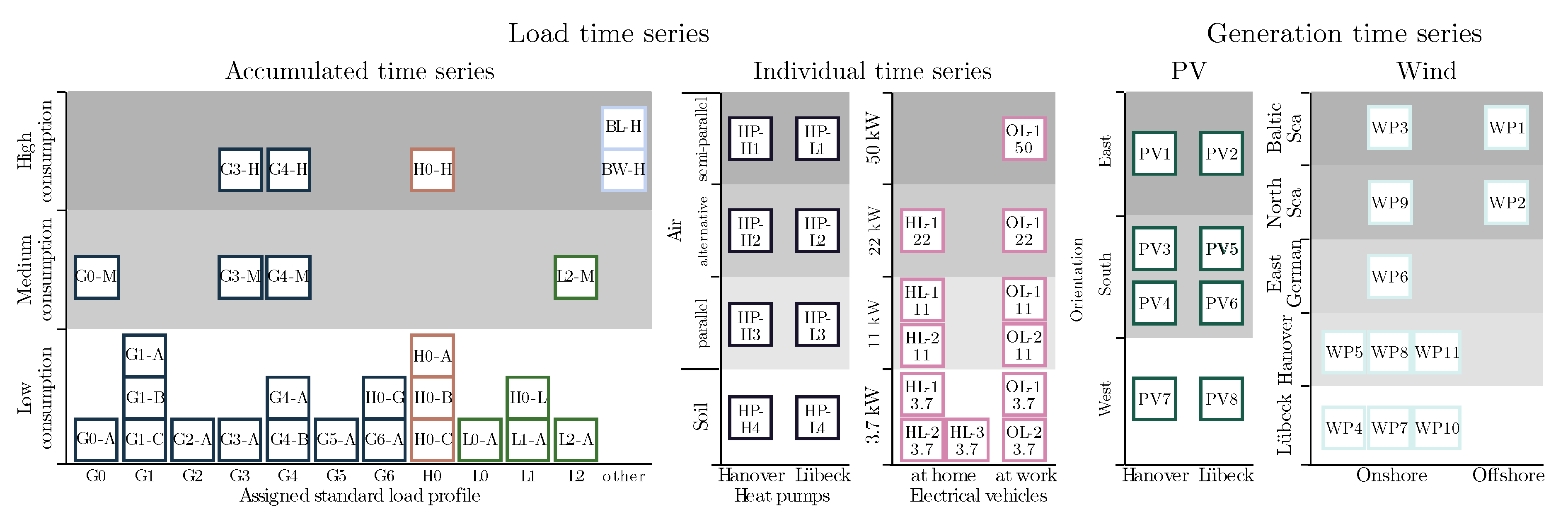
2.2.1. Consumer Time Series

The load time series were distinguished between real measured accumulated, highlighted with a dash, and simulated individual consumers, marked with a solid frame in Figure 1. Commercial enterprises (G), households (H), agricultural holdings (L) and industrial companies (BL/BW) were considered as accumulated consumers, while the provided time series for electric vehicles (EVs) and heat pumps (HPs) were interpreted as individual consumers. For households, 74 smart meter time series provided by the HTW Berlin in the IZES 2010 dataset were evaluated [36]. In terms of the other accumulated consumers, a dataset of more than 2500 anonymized commercial recorded power measurement from the year 2016, provided by the German distribution system operator (DSO) Syna GmbH, was analyzed. All time series came with measured active and reactive power. The aim in the context of SimBench was to provide representative time series extracted from the given measurements. For this purpose, at LV level standard load profiles (SLPs) were used to group commercial customers with similar load shapes into categories. At MV and HV level within certain power ranges individual selections were made.
For the HP time series, we simulated different HP behaviors using annual domestic hot water and space heating demand time series for the German regions around Hanover and Lübeck. The method to generate the demand time series are explained in detail in [37]. The HPs of interest were air and soil HPs operating in a parallel, semi-parallel and alternative operation mode. Different technical restrictions like storage design and blocked periods are considered. In case of the EVs, we generated the time series by randomly combining technical data of currently registered EV types, user mobility behavior based on the “Mobility in Germany” study and charging profiles recorded during a measurement campaign at the Fraunhofer IEE [38,39,40].

2.2.2. Generation Time Series

From LV to HV level, the time series for the photovoltaics (PV), wind and biomass (BM) plants were created with the aid of the agent-based tool SIMONA [41,42]. Real weather data from the German meteorological service (DeutscherWetter Dienst, DWD) were used. At EHV level, a realistic supply task was modeled balancing load and generation. Based on the power plant list of the federal network agency (Bundesnetzagentur, BNetzA) for decommissioned power plants a merit order list determined the power plants in use [28]. The power plant list covered renewable as well as conventional generation plants.

2.2.3. Storage Time Series

In SimBench we distinguished between storages used to maximize self-consumption of generated PV energy and storages used to support grid stability. The storages to maximize self-consumption followed an algorithm storing all excess energy and covering solely customer demand, with their capacity dimensions chosen accordingly. The grid-supporting storages were solely used for curtailment. The curtailed energy added up to 3% of the total energy production.

2.2.4. Aggregated Grid Time Series

Besides consumer time series, the SimBench dataset also provided aggregated grid time series enabling substitutions of the downstream grids. While applicable from the MV to the HV level, SimBench offered the entire German EHV grid, but only two HV grids with specified geographic location. To represent the omitted HV grids, based on a top-down method, aggregated time series were matched to each EHV–HV connection point. For that, a time series of the total power demand in Germany [43] was broken down using information on federal state and municipal level for households, commercial enterprises, agricultural holdings, industrial companies and public transport. In order to reduce the amount of data resembling the power exchange at EHV–HV connection points, the resulting time series were clustered and reduced by a k-means algorithm.

2.2.5. Reactive Power Time Series

In accordance with the predefined study cases, presented in Section 4.1, fixed power factors cos ( φ ) of 1.0 for distributed energy resources (DERs) and of 0.93 for individual loads, storages and omitted HV grids were assumed. The accumulated consumers had real measured reactive power time series.

2.3. Approach for Generating Future Scenarios

The method to generate the future scenarios is intended to cover relevant use cases in grid analysis, planning and operation, such as exemplified in Section 4. Therefore, the scenarios are not suitable to reproduce results found by energy system analyses from models like SCOPE [44] and REMix [45], but rather to address future challenges for the grid management. For the LV, MV and HV level, the method is based on exceeding a certain degree of violations defined for two scenarios projecting the target years 2024 and 2034. This ensures the creation of future grids useful for use cases like topology optimization and conventional grid planning. Violations of interest are overloaded lines and transformers as well as voltage violations.
For this purpose, different producers, consumers and prosumers are randomly distributed into the grids. Furthermore, the load demand per consumer is gradually reduced from 2024 to 2034. In order to prevent unrealistic results, a maximum number of DERs and consumers are set as upper limits.
In contrast to the LV level, for the MV and HV level we define synthetically generated priority areas beforehand. Their individual size and their overall dimension are equivalent to currently existing priority areas and meet the energy policy goals of the state of Hesse [46,47].
The future grids are validated against the results of the integration study for the German state of Hesse [48,49].
Since the development of reliable future scenarios in line with the German EHV grid is out of scope of the SimBench project, only approved high-voltage direct current (HVDC) lines and offshore wind parks are considered [50]. Their projection in the future scenarios just comprise their geographical positions, not respecting their start of operation. Besides the approved changes, the future HV SimBench grids are connected at the two corresponding buses.

3. Overview of the SimBench Dataset

The SimBench dataset comprises the 13 grids introduced in Table 1. In addition, SimBench comes with fitting time series, study cases and combinations of grids of different voltage levels. Furthermore, the future scenarios lead to three variants of all grids. In contrast to other benchmark grids, e.g., available from [2,51], SimBench grids provide switch information and substation configurations. For clarity and a better handling, disconnectors nearby circuit breaker are neglected and a variant with reduced switch information (“no_sw”) is provided as well. Therefore, to clearly label which of these many variants are used, SimBench codes are declared [21]. As in Table 1, SimBench codes consist of a SimBench version number, the considered voltage levels and types of grids, the number of the scenario and an abbreviation whether switches are included in detail.
The grids described in this section are based on general planning and operational principles declared in [30].

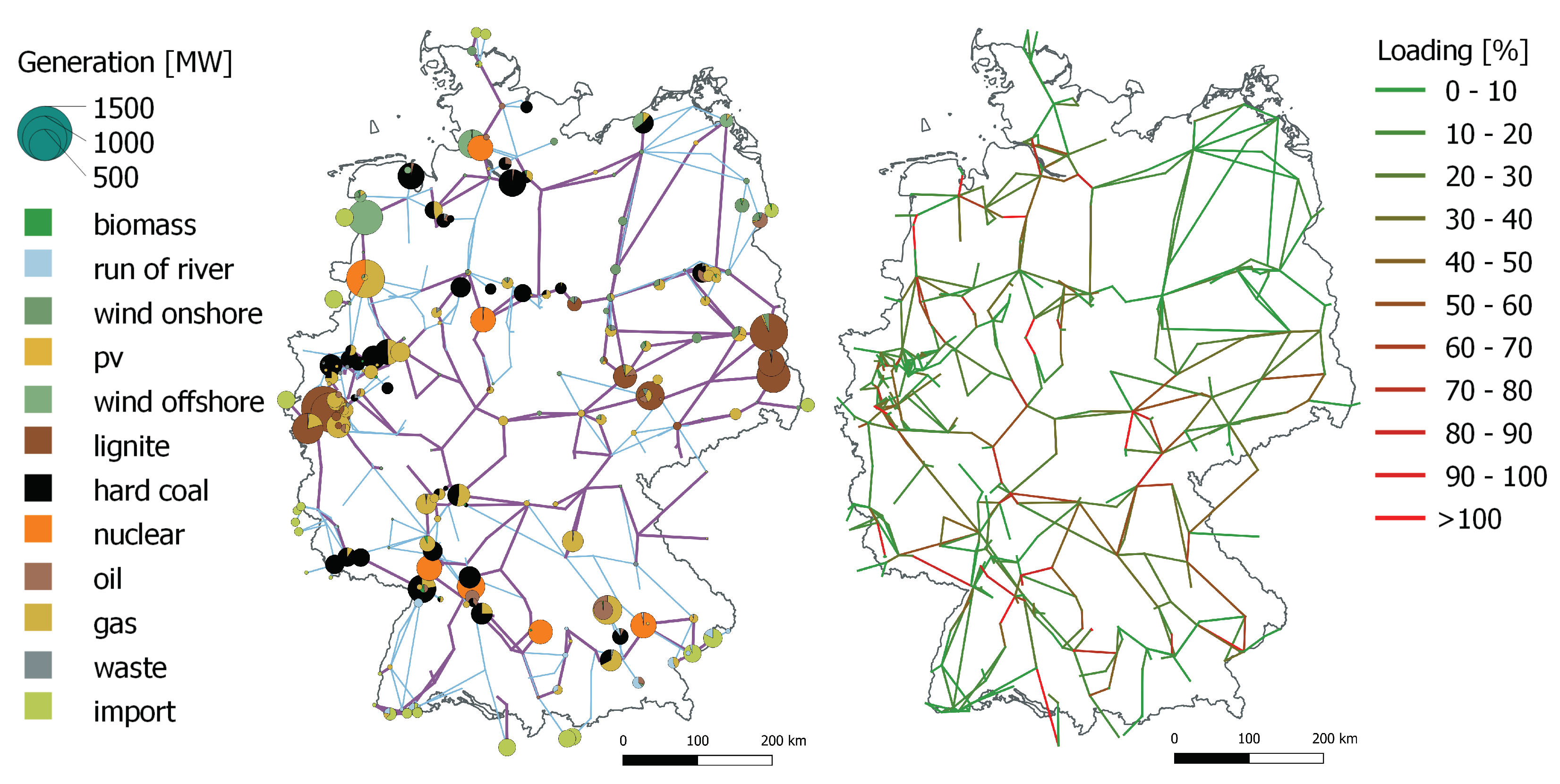
3.1. Extra-High Voltage Grid

The EHV grid model includes 32,425 km of lines, 464 locations, 530 stations and 209 transformers. In addition to the topology of the transmission grid, as described in Section 2.1, the dataset also includes information about the corresponding power supply situation. The geographical distribution of the power plants is depicted in Figure 2 (left). There are large lignite-fired power plants in the Eastern and Western parts of Germany and large gas-fired power plants in the Western and Southern parts of Germany. In addition to the characteristic distribution of onshore wind and PV power plants, the offshore wind farms are also represented by their respective onshore grid connection points.
To validate both the topology and, in particular, the supply situation of the dataset, the power flow results of the SimBench EHV grid have been compared to historical line loadings from the monitoring report of the BNetzA for the year 2017 [52]. For illustration, the power flow result of one time step (2 January 08:00 a.m.) for the Scenario 0 (1-EHV-mixed--0-sw) is depicted in Figure 2 (right). It reflects characteristic congestions in the North-South and North-West direction of Germany. Hence, based on that grid state, use cases such as the determination of remedial measures can be calculated.

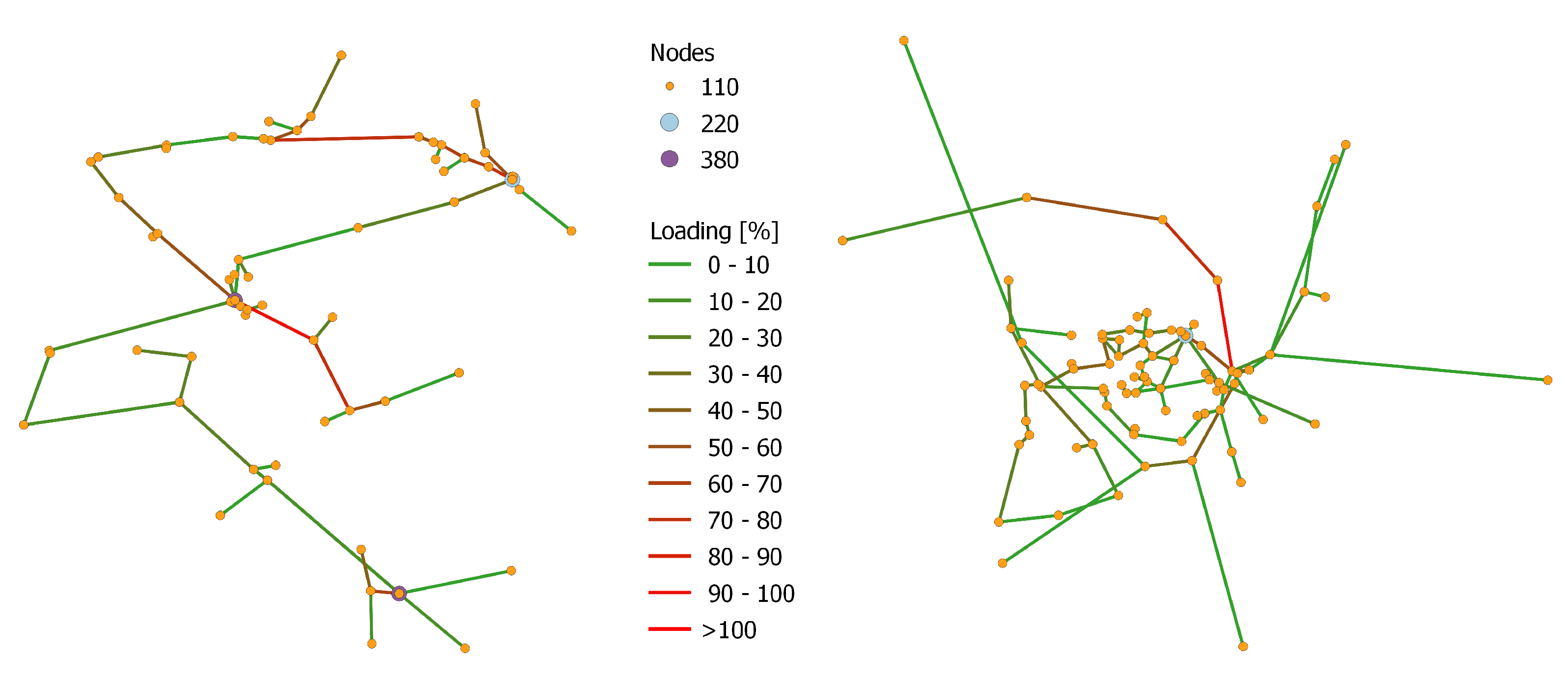
3.2. High Voltage Grids

There are two HV grid models in SimBench. The first is a predominantly rural grid with a high share of overhead lines and the second is a predominantly urban grid with a higher degree of cabling. The connection to the EHV level is realized with high topological flexibility using double busbars while the connection to the MV level includes different substation configurations, as found in real grids [30]. Figure 3 shows the two grid models and the associated supply situation. Based on the distribution of the feeders and loads, it becomes clear that in the predominantly rural grid, there are isolated load centres and the feeders are often installed at a distance from load locations. By contrast, the loads in the predominantly urban grid tend to match the generation sites.
The dimensioning of the grids described in the methodology is carried out with a load flow simulation under consideration of the N-1 criterion. The resulting power flow of both grids is shown in Figure 4 exemplarily for the low load, high generation, extra high wind study case (lW) in the N-1 situation. Considering Figure 4 (left), the high feed-in of the wind power plants combined with low load density results in a high loading of some feeders in the mixed HV grid, predestine this grid e.g., for voltage stability investigations. In Figure 4 (right) of the urban HV grid, it can be seen that the significantly higher load density in the centre of the grid results in a lower line loading since this is close to the generation sites and the EHV substation. The outgoing feeder in the north of the grid is nevertheless highly loaded, since in the high-wind situation, the infeed is higher than the load, as it also includes the infeed of PV power plants.

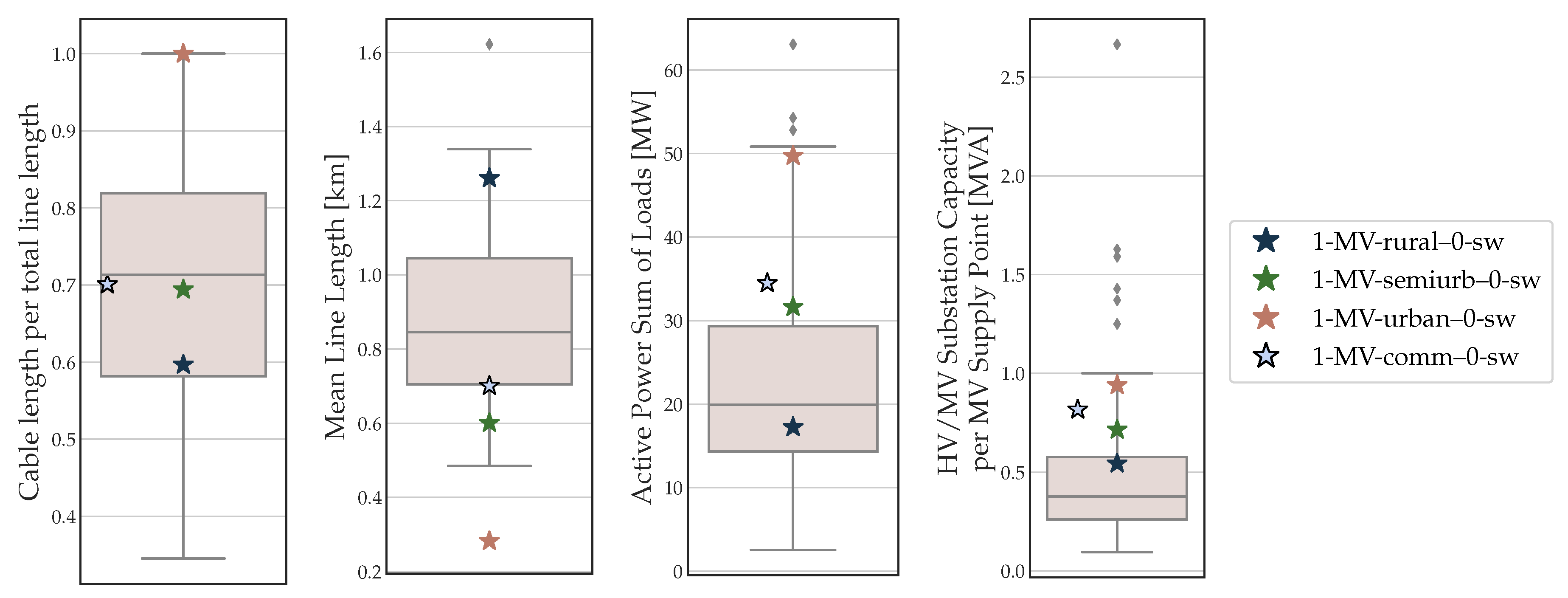
3.3. Medium Voltage Grids

In Figure 5, the MV grid with rural characteristics is illustrated exemplarily. Similar to the LV grids, the data of the MV grids, including the georeferences, are compiled synthetically. The geo-referenced data are fitted to the supplying bus of the overlaying grid. Besides LV grids, the MV grids supply loads and DERs which are directly connected to the MV grids. The grid plot in Figure 5 depicts the open ring topology of the rural MV grid highlighted by the dashed lines. Furthermore, several bus name numbers of the dataset are printed to improve orientation.
As detected by the data analysis of real grids in [20], the cables are usually longer than the overhead lines (OHLs) in SimBench MV grids. To show this, OHLs and cables are illustrated by different colors. In addition, the ratio of these both types of lines is depicted in Figure 6 (left). In this figure, the four SimBench MV grids are compared to the data of 74 separately operated real MV grids. The grids are spread over five DSOs and include a line length sum of about 11,000 km. The real grids data are figured by boxplots. Besides the ratio of OHLs and cables, three further parameters are depicted in Figure 6. On the one hand, they show that the SimBench MV grids comprise a large percentage of the real grids distribution. On the other hand, the mean line length of the urban MV grid is the only outlying value. This is accepted since the analyzed set of real grids does not include a complete urban grid.
All grids supplied by the SimBench MV grids correspond to the SimBench LV grids. Since weakly loaded, not challenging LV grids are not included in SimBench, most markers of the SimBench MV grids lie in the upper half of the real grid distribution of the active power sum of loads and the HV/MV substation capacity per MV supply point. However, according to the predefined study cases, which are described in Section 4.1, the SimBench MV grids cause no violations but reach some limits nearby. As stated in literature and observed in real grids, the most challenging case for the urban SimBench MV grid is the high load, low generation case (hL). The rural SimBench MV grid reaches voltage limits in the low load, high generation cases (lW, lPV).

3.4. Low Voltage Grids

There are six LV grid models in SimBench, for each cluster (see Section 2.1.3) one model [34]. As shown exemplarily in Figure 7, each grid model reveals a radial topology, since this is the dominant structure at the LV level. The equipment used in the models is:
  • Transformers ( S r ): {160, 400, 630} kVA
  • Cables: NAYY 4 x {150, 240} mm 2
The model called LV1 is the most rural SimBench LV grid with mainly agricultural holdings as consumers. By contrast, the other two rural grids (LV2, LV3) predominantly supply household loads with individual commercial consumers. Since these represent villages and rural settlements, the number of consumers and thus also buses is higher than in LV1. The two semi-urban grids (LV4, LV5) represent the structures of smaller cities and suburbs of larger cities. In order to map small multi-family houses, semi-urban individual consumers have a higher power demand compared to the rural grids. In the urban grid (LV6), multi-family house loads are divided into several individual loads and thus modeled separately. This is meant to prevent unrealistic load peaks especially when calculating with time series.
Within the evaluation in [34], 180 real grids from Germany have been compared to the SimBench LV grids with regard to the number of consumers, the active power of consumers and line length. The evaluation has shown that these LV grids are well able to represent the real grids classified by clusters.

3.5. Load, Generation, Storage and Aggregated Grid Time Series

Instead of presenting all described time series, here we concentrate on the most important results.
The SimBench dataset provides 27 accumulated load time series and a total of 20 individual ones, comprised of 12 for EVs and eight for HPs. The overview of the accumulated time series in Figure 8 (left) [35] show the categorized time series in accordance to the SLP types and their total consumption.
As illustrated in the middle right of the figure, we distinguish the EV between two charging positions, i.e., household charging stations and workplace charging stations, and different nominal power configurations. In addition to these, EV time series for 101.4 kW and 507 kW at MV and HV level exist. However, these are solely the aggregations of all workplace time series differently scaled. Besides EV time series, the SimBench dataset provides HP time series for the two locations of the SimBench HV grids. As shown in Figure 8, these vary in different operating modi and heat sources.
For DERs, synthetic time series are provided in the SimBench dataset. These include eight for PV, eleven for wind parks and five for BM plants. The plant locations have been distributed geographically in order to take locally varying weather conditions in the time series into account. As with the HPs, locations in the region around Hanover and Lübeck were chosen on the basis of the HV grids. For the time series for offshore wind farms, locations in the North Sea and Baltic Sea have been selected. In addition to geographical locations, the PV time series also distinguish between different orientations. Furthermore, three anonymized time series for hydroelectric power plants are available.
Besides consumers and producers, 48 prosumers in the form of battery storage time series are also part of the SimBench dataset. 40 time series are self-consumption maximizing and eight time series run in a manner beneficial to the grid.
On top, SimBench also offers 30 time series for the EHV-HV connection points, which are subdivided into 28 time series resembling the consumption within Germany and two time series standing for the demand of the neighboring countries.

3.6. Future Scenarios

Two future grids are implemented for each SimBench grid. Instead of evaluating all differences of each grid, this section focuses on examples highlighting general features.
The implemented method ensures a broad spectrum of possible grid planning, operation and analysis challenges. In Figure 9, the heat map of the LV3 grid for example emphasizes that in Scenario 1 for the low load, high generation and extra high PV study case (lPV) mainly new installed DERs cause overvoltages, whereas in Scenario 2 for the high load, low generation generation study case (hL) an increased number of new individual consumers causes undervoltages. On top, higher transformer and line loadings are more prominent in Scenario 2.
While in LV grids only the pre-existing nodes are used for new installations, in MV and HV grids the topology is slightly changed by adding new buses. These buses connect the priority areas with the grids. In SimBench, new DERs within priority areas are connected to the new buses. However, if they exceed a nominal power of 8.0 MW, they are directly connected to the transformer station.
The EHV future scenarios include the HVDC lines ALEGro, A-Nord, SuedLink and SuedOstLink, Ultranet. In contrast to that, the new off-shore wind plants, installed in Northern Germany, do not change the topology, as they are connected to already existing grid nodes.

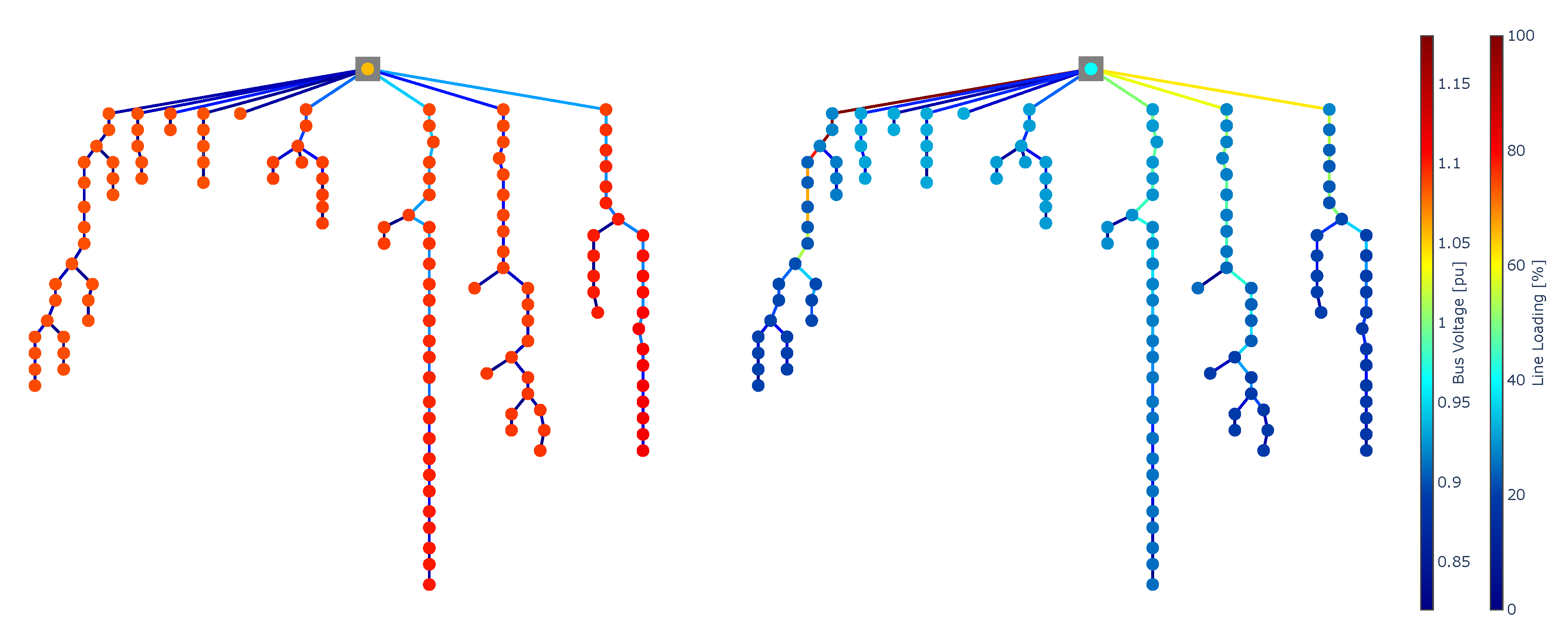
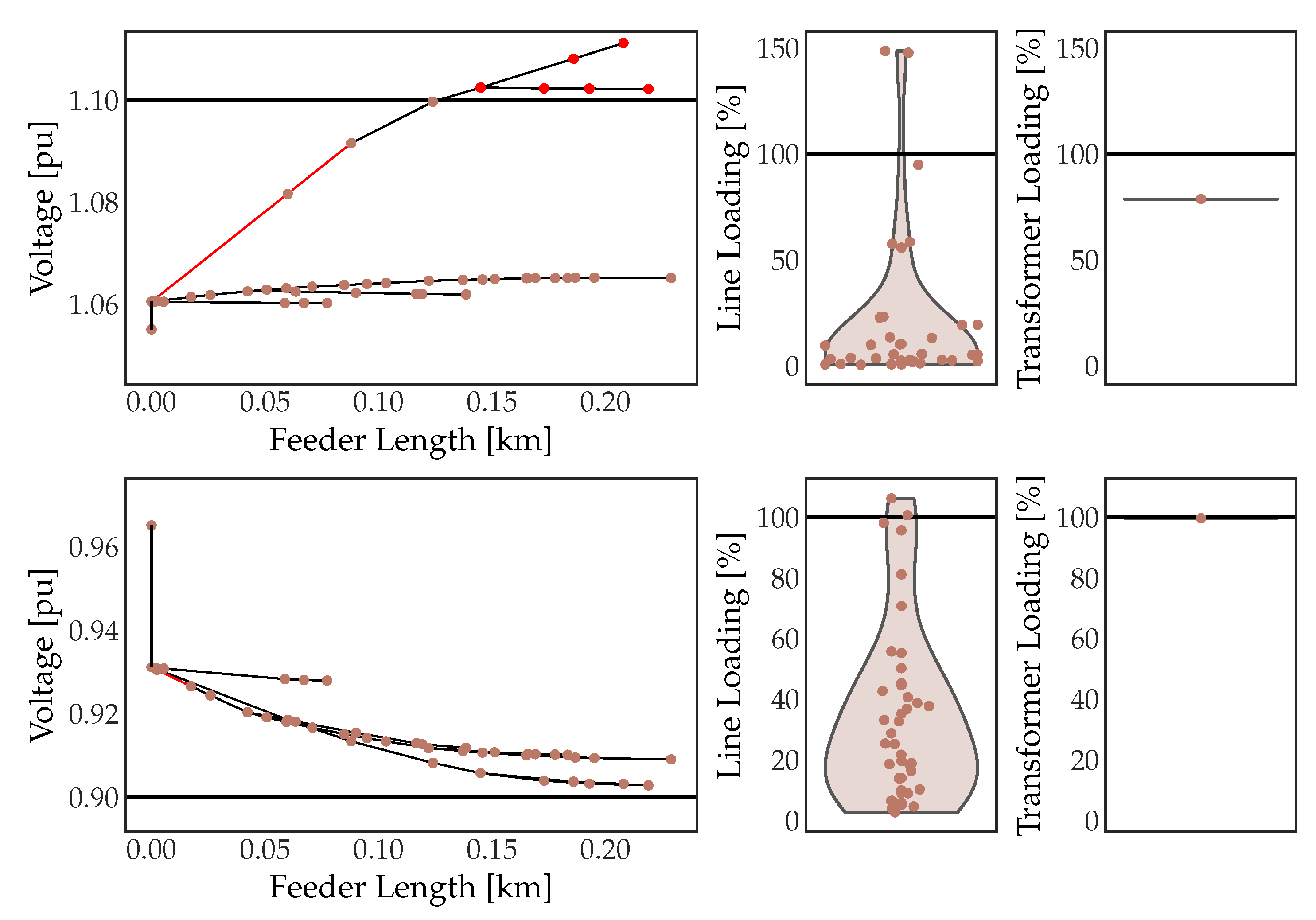
4. Application Example of the SimBench Dataset

In this section, a grid expansion planning use case is presented to exemplify how to use the SimBench dataset. Therein, the predefined study cases [30], the load and generation time series [35] and the future scenarios are applied. This comparison of different algorithms illustrates the ability to use the SimBench dataset for benchmarking.

4.1. Predefined Study Cases and Time Series

The study cases include voltage, line loading and transformer loading limits as well as scalings for load and generation powers [30]. Applying this to the LV grid from Figure 7 “1-LV-semiurb4--2-no_sw”, the grid state as drawn in Figure 10 results. In this figure, each dot represents a bus voltage, a line loading or a transformer loading. On the left, these are aligned with respect to the distance to the supplying MV bus and linked by the connecting lines and transformers. Here, overloadings and voltage violations are highlighted in red. The other diagrams of Figure 10 include violin plots of the loadings. The horizontal black lines illustrate the operational limits. To conclude, at the low load, high generation, extra-high PV generation (lPV, top) study case six bus voltages exceed the upper voltage limit and in both figured study cases two lines violate the loading limit.
Similarly, the power flow situation of each time step is obtained by multiplying the specified peak power values of the loads and DERs by the scaling factors of the time step. Simulating the “1-LV-semiurb4--2-no_sw” grid with the full year time series, 143 of the 35,136 time steps show any violations.

4.2. Applied Algorithms and Grid Planning Use Case

In this use case, two different automated grid expansion algorithms are compared, again using the “1-LV-semiurb4--2-no_sw” grid. Both are based on heuristic planning approaches.
The first algorithm, referred to as Algorithm A, corresponds to the methodology published in [53]. It is supposed to map the manual planning process as it occurs in reality. The methodology can be divided into the following steps:
  • Implement a forecast scenario
  • Power flow analysis
  • Optimization of the transformer tap position
  • Grid expansion
  • Investment evaluation
First, a supply task is implemented, based on a forecast scenario. This includes integrating individual plants and loads into the grid model for examination. Subsequently, the grid situation is assessed with a power flow analysis in order to identify limit violations. If violations occur, e.g., thermal overloads, the tap position of the transformer is adjusted and, if necessary, grid expansion is carried out. This process is iterative and continues until there are no more violations. In a final step, the resulting capital expenditures are determined.
A slight adaptation to what is presented in [53] is made for the use with SimBench. Besides the grid model, Algorithm A usually uses load and generation forecasts to estimate a forecast scenario. In the SimBench dataset, however, designated future scenarios are already available, eliminating the need for such forecasts. Taking this into account, the remaining relevant steps of Algorithm A are evaluating voltage and loading violations, optimizing the transformer tap position, reinforcing and expanding the grid if required and finally evaluating the investment.
Algorithm B [54,55] basically runs according to the following iterative procedure to improve the current best solution:
  • Generate new candidate solutions from the actual solution and (randomly) select one
  • Evaluate an acceptance criterion, whether the new solution should replace the previous solution or be rejected
While Algorithm A is rule-based, different variants of generating new candidates via a so-called neighbourhood function are applicable within Algorithm B. Here we use a hill climbing algorithm which searches for new candidate solutions by adding or replacing a measure from Table 2. The implemented criterion accepts new solutions if the cost function is reduced. To be able to start from the initial state of the grid and to accept additional measures that improves the solution but still do not eliminate all violations, the cost function includes the capital expenditures as well as the degree of occurring violations. In this way, the heuristic can also handle non-feasible solution spaces. The iterative search can be stopped in various ways, e.g., when a time period or number of iterations is exceeded or the cost function reaches a certain value. However in this simple example, there is no need to stop before all possible measures are evaluated.
The task for Algorithm A and B is to solve occurring voltage violations and overloadings using the available measures, summarized in Table 2. The costs of the available measures are similar to state-of-the-art German DER integration studies assumptions [48,49,57]. The comparison includes three variants of running Algorithm B: B1 has the same set of available measures like A. With B2 we also present the possibility to use a second standard line type. B3 investigates the critical grid states of predetermined 143 time steps instead of both relevant study cases “hL” and “lPV”.

4.3. Comparison of the Performance of the Applied Algorithms

Table 3 presents the measures and the associated costs proposed by running the algorithms. These can be easily explained with Figure 10. The four overloaded lines shown in the figure are the lines reinforced by B1 and B2. The reinforcement of these lines also solves the voltage issues. The most significant difference in cost between Algorithm A and B1 is that A proposes to reinforce the original transformer. This can be explained by inaccuracies in the calculation of the power flow. In Algorithm A, the transformer loading is marginally above 100%, thus violating the limit value, while in Algorithm B the loading is just below 100%. By reinforcing the transformer, Algorithm A does not need to reinforce the line from bus 5 to 26.
Using a second line standard type with a larger cross-section (400 mm2), B2 does not require parallel lines. Usually, however, DSOs decide against the measures of B2 because of higher operational expenses of maintaining a second LV standard line type.
B3 is capable of solving all issues by merely reinforcing two lines which costs 25% less than with B1. Furthermore, while the bus voltages that result from the study cases already fill out the complete voltage range in Figure 10, B3 finds solutions with four different transformer tap positions for the critical grid states. However, due to the long service life of the components, DSOs design grids for decades instead of one specific year. In addition to the uncertainties of the considered time series within a time series-based grid planning, the computing effort to run algorithms with time series is higher because of the number of time steps to be considered. In this simple study, the median computing time (Run with Python 3.6.8 on an Intel(R) Core(TM) i7-4712MQ CPU with 2.3 GHz, 16 GB RAM and SSD) running B3 is, as depicted in Figure 11, 4.79 s instead of 2.13 s (B1) and 1.28 s (B2). (Algorithm A, which also checks measures beyond those relevant in this study case, is performed on another customary laptop so that the computing time of about 12 s to 15 s is not fairly comparable and thus not shown in Figure 11).
To sum up, using the SimBench dataset the two exemplarily run, automated grid planning algorithms and their variants can be compared appropriately without additional data.

5. Conclusions

SimBench, the open-source dataset of electric steady-state grid models can be used as a benchmark for various use cases. The dataset has been validated regarding the suitability of the data with simulation and has deliberately determined grid states including suitable dimensioning of grid assets. The dataset can be used for several purposes:
Firstly, being specific for Germany, the benchmark dataset is especially applicable for power grid analyses in Central Europe. However, the detailed description of the dataset compilation in this paper should also make it possible to extend such publicly available benchmark datasets to other geographical areas. However, even without any such extensions, it offers some helpful features for applications outside this area: Compared to older grid models, SimBench offers grids that have significantly higher large shares of renewables useful for studies with recent technologies. Grids in numerous countries may be on course for a similar share of renewables, which would make the SimBench grids promising candidates for the investigation of future challenges. Due to the three sets of scenarios with different renewable energy penetration, the SimBench dataset makes it possible to choose the scenario with the most suitable amount of renewables for a given investigation.
Secondly and independent of the geographical area of application, the SimBench dataset makes it possible to comprehensively model grids spanning several voltage levels. As the SimBench dataset comprises grids from the LV to the EHV level, it allows to investigate the effects of changes at one voltage level on the other ones.
Thirdly, the SimBench dataset provides fitting load, generation and storage time series, which extend the reproducibility of SimBench-based power system analyses and the applicable use cases. This is complemented by the provided switch information and substation configurations—fundamental information for use cases like N-1 analysis, which have rarely been part of existing datasets.
Summing up, the SimBench dataset, which includes valuable grids of four voltage levels and three different scenarios as well as extensive time series data, can be downloaded freely from a public website [1], making the dataset a readily available resource for the benchmarking of methods for power system analysis. As stated before, SimBench aims to include grids with realistic challenges for various use cases to provide an appropriate dataset as a benchmark for comparisons, e.g., for operation strategies or, as presented, for planning algorithms. To be user friendly, the dataset is available in four different data formats (pandapower, PowerFactory, INTEGRAL and CSV) and its corresponding website includes a GUI for selecting and downloading suitable parts of the dataset, clearly labeled by SimBench codes. Therefore, SimBench attempts to make a contribution towards providing datasets to facilitate reproducible applications in a broad range of power grid analyses.

Author Contributions

Conceptualization, methodology, visualization, software, validation and data curation: S.M., D.S., S.R.D. and A.K.; writing–original draft preparation: S.M., D.S., S.R.D., A.K. and L.-P.L.; writing–review and editing: all authors; supervision: L.-P.L., C.R., A.M. and M.B.; project administration: L.-P.L.; funding acquisition: C.R., A.M. and M.B. All authors have read and agreed to the published version of the manuscript.

Funding

This work was supported by the German Federal Ministry for Economic Affairs and Energy and the Projektträger Jülich GmbH (PTJ) within the framework of the project SimBench (FKZ: 0325917). The authors are solely responsible for the content of this publication.

Acknowledgments

The authors would like to thank all colleagues who contributed to the project SimBench. We would also like to acknowledge the system operators for their active participation, helpful feedback and provision of grid data. These were DREWAG NETZ GmbH, Energie Netz Mitte GmbH, ENSO NETZ GmbH, Netze BW GmbH, Syna GmbH and Westnetz GmbH.

Conflicts of Interest

The authors declare no conflict of interest. The funders had no role in the design of the study; in the collection, analyses, or interpretation of data; in the writing of the manuscript, or in the decision to publish the results.

References

  1. Project SimBench—Simulation Data Base for a Consistent Comparison of Innovative Solutions in the Field of Grid Analysis, Grid Planning and Grid Operation Management. Available online: www.simbench.net/en (accessed on 5 July 2018).
  2. Christie, R.D. Power Systems Test Case Archive; University Of Washington: Washington, DC, USA, 1999; Available online: http://www2.ee.washington.edu/research/pstca/ (accessed on 20 June 2018).
  3. Schneider, K.P.; Mather, B.A.; Pal, B.C.; Ten, C.; Shirek, G.J.; Zhu, H.; Fuller, J.C.; Pereira, J.L.R.; Ochoa, L.F.; de Araujo, L.R.; et al. Analytic Considerations and Design Basis for the IEEE Distribution Test Feeders. IEEE Trans. Power Syst. 2018, 33, 3181–3188. [Google Scholar] [CrossRef]
  4. Strunz, K.; Hatziargyriou, N.; Andrieu, C. Benchmark systems for network integration of renewable and distributed energy resources. Cigre Task Force C 2009, 6, 78. [Google Scholar]
  5. Meinecke, S.; Thurner, L.; Braun, M. Review and Classification of Published Electric Steady-State Power Distribution System Models. 2020. Available online: https://arxiv.org/abs/2005.06167 (accessed on 14 May 2020).
  6. Bialek, J.; Ciapessoni, E.; Cirio, D.; Cotilla-Sanchez, E.; Dent, C.; Dobson, I.; Henneaux, P.; Hines, P.; Jardim, J.; Miller, S.; et al. Benchmarking and validation of cascading failure analysis tools. IEEE Trans. Power Syst. 2016, 31, 4887–4900. [Google Scholar] [CrossRef] [Green Version]
  7. Mateo, C.; Prettico, G.; Gómez, T.; Cossent, R.; Gangale, F.; Frías, P.; Fulli, G. European representative electricity distribution networks. Electr. Power Energy Syst. 2018, 99, 273–280. [Google Scholar] [CrossRef]
  8. Pilo, F.; Pisano, G.; Scalari, S.; Canto, D.D.; Testa, A.; Langella, R.; Caldon, R.; Turri, R. ATLANTIDE—Digital archive of the Italian electric distribution reference networks. In Proceedings of the CIRED 2012 Workshop: Integration of Renewables into the Distribution Grid, Lisbon, Portugal, 29–30 May 2012; pp. 1–4. [Google Scholar] [CrossRef]
  9. Celli, G.; Pilo, F.; Pisano, G.; Soma, G.G. Reference scenarios for Active Distribution System according to ATLANTIDE project planning models. In Proceedings of the 2014 IEEE International Energy Conference (ENERGYCON), Cavtat, Croatia, 13–16 May 2014; IEEE: Piscataway, NJ, USA, 2014; pp. 1190–1196. [Google Scholar]
  10. Bracale, A.; Caldon, R.; Celli, G.; Coppo, M.; Dal Canto, D.; Langella, R.; Petretto, G.; Pilo, F.; Pisano, G.; Proto, D.; et al. Analysis of the Italian distribution system evolution through reference networks. In Proceedings of the 2012 3rd IEEE PES Innovative Smart Grid Technologies Europe (ISGT Europe), Berlin, Germany, 14–17 October 2012; IEEE: Piscataway, NJ, USA, 2012; pp. 1–8. [Google Scholar]
  11. Subcommittee, P.M. IEEE Reliability Test System. IEEE Trans. Power Appar. Syst. 1979, PAS-98, 2047–2054. [Google Scholar] [CrossRef]
  12. Grigg, C.; Wong, P.; Albrecht, P.; Allan, R.; Bhavaraju, M.; Billinton, R.; Chen, Q.; Fong, C.; Haddad, S.; Kuruganty, S.; et al. The IEEE Reliability Test System-1996. A report prepared by the Reliability Test System Task Force of the Application of Probability Methods Subcommittee. IEEE Trans. Power Syst. 1999, 14, 1010–1020. [Google Scholar] [CrossRef]
  13. Josz, C.; Fliscounakis, S.; Maeght, J.; Panciatici, P. AC Power Flow Data in MATPOWER and QCQP Format: iTesla, RTE Snapshots, and PEGASE. 2016. Available online: https://arxiv.org/abs/1603.01533 (accessed on 12 May 2020).
  14. Fliscounakis, S.; Panciatici, P.; Capitanescu, F.; Wehenkel, L. Contingency Ranking With Respect to Overloads in Very Large Power Systems Taking Into Account Uncertainty, Preventive, and Corrective Actions. IEEE Trans. Power Syst. 2013, 28, 4909–4917. [Google Scholar] [CrossRef] [Green Version]
  15. Marten, F.; Löwer, L.; Töbermann, J.C.; Braun, M. Optimizing the reactive power balance between a distribution and transmission grid through iteratively updated grid equivalents. In Proceedings of the Power Systems Computation Conference (PSCC), Wrocław, Poland, 18–22 August 2014; pp. 1–7. [Google Scholar]
  16. Schäfer, F.; Menke, J.H.; Marten, F.; Braun, M. Time Series Based Power System Planning Including Storage Systems and Curtailment Strategies. In Proceedings of the CIRED 2019 25th International Conference on Electricity Distribution, Madrid, Spain, 3–6 June 2019; AIM: Madrid, Spain, 2019. [Google Scholar]
  17. Schäfer, F.; Menke, J.H.; Braun, M. Comparison of Meta-Heuristics for the Planning of Meshed Power Systems. 2020. Available online: https://arxiv.org/abs/2002.03619 (accessed on 12 May 2020).
  18. Larscheid, P.; Klettke, A.; van Leeuwen, T.; Meinecke, S.; Moser, A. Einfluss der Modellierungsgenauigkeit des Höchstspannungsnetzes auf die Simulation von Hochspannungsnetzen [Impact of the Extra High Voltage Grid Modeling Accuracy on the Simulation of High Voltage Grids]. 15. Symposium Energieinnovation. 2018. Available online: https://www.tugraz.at/fileadmin/user_upload/Events/Eninnov2018/files/lf/Session_D4/541_LF_Klettke1.pdf (accessed on 24 May 2020).
  19. Liu, Z.; Wende-von Berg, S.; Banerjee, G.; Bornhorst, N.; Kerber, T.; Maurus, A.; Braun, M. Adaptives Statisches Netzäquivalent Mit künstlichen Neuronalen Netzen [Adaptive Static Network Equivalent with artificial Neuronal Networks]. 16. Symposium Energieinnovation. 2020. Available online: https://www.tugraz.at/events/eninnov2020/nachlese/download-beitraege/stream-d/#c279406 (accessed on 24 May 2020).
  20. Meinecke, S.; Bornhorst, N.; Braun, M. Power System Benchmark Generation Methodology. In Proceedings of the NEIS-Conference, Hamburg, Germany, 20 September 2018. [Google Scholar]
  21. Meinecke, S.; Drauz, S.; Klettke, A.; Sarajlic, D.; Sprey, J.; Spalthoff, C.; Kittl, C.; Braun, M.; Moser, A.; Rehtanz, C. SimBench Documentation—Electric Power System Benchmark Models; Technical Report EN-1.0.0; University of Kassel, Fraunhofer IEE, RWTH Aachen University, TU Dortmund University: Kassel, Germany, 2020. [Google Scholar]
  22. Thurner, L.; Scheidler, A.; Schäfer, F.; Menke, J.; Dollichon, J.; Meier, F.; Meinecke, S.; Braun, M. Pandapower—An Open-Source Python Tool for Convenient Modeling, Analysis, and Optimization of Electric Power Systems. IEEE Trans. Power Syst. 2018, 33, 6510–6521. [Google Scholar] [CrossRef] [Green Version]
  23. DIgSILENT GmbH. DIgSILENT PowerFactory. Version 2017. Available online: https://www.digsilent.de/en/news.html (accessed on 20 January 2020).
  24. FGH GmbH. INTEGRAL. Available online: https://www.fgh-ma.de/de/ueber-uns/fgh-organisation/fgh-gmbh (accessed on 20 January 2020).
  25. OpenStreetMap. About Openstreetmap—Openstreetmap Wiki. Available online: https://wiki.openstreetmap.org/wiki/Main_Page (accessed on 1 July 2018).
  26. Reiners, D. Flosm Powergrid. Available online: http://www.flosm.de/en/powergrid.html (accessed on 1 July 2018).
  27. Matke, C.; Medjroubi, W.; Kleinhans, D. SciGRID—An Open Source Reference Model for the European Transmission Network (v0.2). 2016. Available online: http://www.scigrid.de (accessed on 12 May 2018).
  28. Bundesnetzagentur. Marktstammdatenregister [Market Data Register]. Available online: https://www.marktstammdatenregister.de/MaStR/Einheit/Einheiten/OeffentlicheEinheitenuebersicht (accessed on 31 May 2019).
  29. DESTATIS—Statistisches Bundesamt [German Federal Statistical Office]. Available online: https://www.destatis.de/EN/Home/_node.html (accessed on 1 July 2018).
  30. Meinecke, S.; Klettke, A.; Sarajlic, D.; Dickert, J.; Hable, M.; Fischer, F.; Braun, M.; Moser, A.; Rehtanz, C. General Planning and Operational Principles in German Distribution Systems Used for SimBench. In Proceedings of the CIRED 25th International Conference on Electricity Distribution, Madrid, Spain, 3–6 June 2019. [Google Scholar]
  31. Klettke, A.; van Leeuwen, T.; Flörkemeier, S.; Moser, A. Generierung von Benchmark—Modellnetzen in der Hochspannungsebene auf Basis öffentlich verfügbarer Daten [Generation of high Voltage Benchmark Grids Based on Publicly Accessible Data]. 10. Internationale Energiewirtschaftstagung an der TU Wien. 2017. Available online: https://simbench.de/wp-content/uploads/2019/02/IEWT2017_lf_Klettke.pdf (accessed on 24 May 2020).
  32. Kittl, C.; Sarajlić, D.; Rehtanz, C. k-means based identification of common supply tasks for low voltage grids. In Proceedings of the 2018 IEEE PES Innovative Smart Grid Technologies Conference Europe (ISGT-Europe), Sarajevo, Bosnia and Herzegovina, 21–25 October 2018; pp. 1–5. [Google Scholar] [CrossRef]
  33. Kays, J.; Seack, A.; Smirek, T.; Westkamp, F.; Rehtanz, C. The Generation of Distribution Grid Models on the Basis of Public Available Data. IEEE Trans. Power Syst. 2017, 32, 2346–2353. [Google Scholar] [CrossRef]
  34. Sarajlić, D.; Rehtanz, C. Low Voltage Benchmark Distribution Network Models Based on Publicly Available Data. In Proceedings of the IEEE PES Innovative Smart Grid Technologies Europe (ISGT-Europe), Bucharest, Romania, 29 September–2 October 2019; pp. 1–5. [Google Scholar] [CrossRef]
  35. Spalthoff, C.; Sarajlić, D.; Kittl, C.; Drauz, S.; Kneiske, T.; Rehtanz, C.; Braun, M. SimBench: Open source time series of power load, storage and generation for the simulation of electrical distribution grids. In Proceedings of the International ETG Congress, Esslingen, Germany, 28–29 November 2019. [Google Scholar]
  36. Tjaden, T.; Bergner, J.; Weniger, J.; Quaschning, V. Repräsentative elektrische Lastprofile für Wohngebäude in Deutschland auf 1-sekündiger Datenbasis [Representative Electrical Load Profiles for Residential Buildings in Germany Based on 1-Second Data]. 2015. Available online: https://doi.org/10.13140/RG.2.1.5112.0080 (accessed on 18 July 2018).
  37. Drauz, S. Synthesis of A Heat and Electrical Load Profile for Single and Multi-Family Houses Used for Subsequent Performance Tests of A Multi-Component Energy System. Master’s Thesis, RWTH Aachen University, Aachen, Germany, 2016. [Google Scholar]
  38. Follmer, R.; Gruschwitz, D.; Jesske, B.; Quandt, S.; Lenz, B.; Nobis, C.; Köhler, K.; Mehlin, M. Mobilität in Deutschland 2008 [Mobility in Germany]; Technical report; infas Institut für angewandte Sozialwissenschaft GmbH; Deutsches Zentrum für Luft- und Raumfahrt e.V: Cologne, Germany, 2010. [Google Scholar]
  39. Prior, J. Testverfahren zur Bestimmung des Elektrischen Verhaltens von Batteriesystemen in Elektrofahrzeugen [Test Method to Determine the Electric Behaviour of Battery Systems in Electric Vehicles]. Ph.D. Thesis, University Kassel, Kassel, Germany, 2017. [Google Scholar]
  40. Statista. Neuzulassungen von Elektroautos nach Marke/Modellreihe bis 2018 [New Registrations of Electric Vehicles by Brand/model Line Until 2018]. Available online: https://de.statista.com/statistik/daten/studie/224041/umfrage/neuzulassungen-von-elektroautos-nach-marke-modellreihe/ (accessed on 14 April 2020).
  41. Kays, J.; Rehtanz, C. Planning process for distribution grids based on flexibly generated time series considering RES, DSM and storages. IET Gener. Transm. Distrib. 2016, 10, 3405–3412. [Google Scholar] [CrossRef]
  42. Kays, J.; Seack, A.; Häger, U. The potential of using generated time series in the distribution grid planning process. In Proceedings of the CIRED 23rd International Conference on Electricity Distribution, Lyon, France, 15–18 June 2015. [Google Scholar]
  43. ENTSO-E. Historical data (until December 2015)—Consumption Data: Hourly Load Values 2006–2015. 2015. Available online: https://www.entsoe.eu/data/data-portal/ (accessed on 8 August 2019).
  44. Fraunhofer IEE. Sektorübergreifende Einsatz- und Ausbauoptimiertung für die Analysen des Zukünftigen Energieversorgungssystems [Multi-Sectors Deployment and Expansion Optimization for the Analyses of the Future Energy Supply System]. Available online: https://www.iee.fraunhofer.de/content/dam/iee/energiesystemtechnik/de/Dokumente/Broschueren/2018_F_SCOPE_Einzelseiten.pdf (accessed on 17 April 2020).
  45. Scholz, Y. Renewable Energy Based Electricity Supply at Low Costs. Ph.D. Thesis, University Stuttgart, Stuttgart, Germany, 2012. [Google Scholar]
  46. Regionalversammlung Mittelhessen. Anhang 2—Steckbriefe der im Teilregionalplanentwurf Ausgewiesenen Vorranggebiete zur Nutzung der Windenergie (VRG WE) [Appendix 2 —Briefings of Priority Areas for the Use of Wind Energy (VRG WE) Identified in the Sub-Regional Plan Draft]; Technical Report; Regierungspräsidium Gießen, Dezernat 31: Gießen, Germany, 2012. [Google Scholar]
  47. van den Busch, U.; Gauler, A.; Müller, H.; Frings, K.; Petkova, G. Energiewende in Hessen—Monitoringbericht 2016 [Energy Transition in Hesse—Monitoring Report 2016]; Technical Report; Hessisches Ministerium für Wirtschaft, Energie, Verkehr und Landesentwicklung: Wiesbaden, Germany, 2016.
  48. Scheidler, A.; Bolgaryn, R.; Ulffers, J.; Dasenbrock, J.; Horst, D.; Gauglitz, P.; Pape, C.; Becker, H.; Braun, M. DER Integration study for the German state of hesse—Methodology and key results. In Proceedings of the CIRED 25th International Conference on Electricity Distribution, Madrid, Spain, 3–6 June 2019. [Google Scholar]
  49. Braun, M.; Krybus, I.; Becker, H.; Bolgaryn, R.; Dasenbrock, J.; Gauglitz, P.; Horst, D.; Pape, C.; Scheidler, A.; Ulffers, J. Veteilnetzstudie Hessen 2024-2034 [Der Integration Study for The German State of Hesse]; Technical Report; BearingPoint GmbH and Fraunhofer IEE: Frankfurt am Main, Germany, 2018. [Google Scholar]
  50. 50Hertz Transmission GmbH and Amprion GmbH and TenneT TSO GmbH and TransnetBW GmbH. In Netzentwicklungsplan Strom 2030, Version 2019 [Network Development Plan of Electricity 2030, Version 2019]; Technical Report; CB.e Clausecker | Bingel AG: Berlin, Germany, 2019.
  51. Zimmerman, R.D.; Murillo-Sánchez, C.E.; Thomas, R.J. MATPOWER: Steady-state operations, planning, and analysis tools for power systems research and education. IEEE Trans. Power Syst. 2011, 26, 12–19. [Google Scholar] [CrossRef] [Green Version]
  52. Bundesnetzagentur. Monitoringbericht 2017 [Monitoring Report 2017]. Available online: https://www.bundesnetzagentur.de/SharedDocs/Mediathek/Monitoringberichte/Monitoringbericht2017.pdf?_blob=publicationFile&v=4 (accessed on 14 April 2020).
  53. Wagner, C.; Kittl, C.; Kippelt, S.; Rehtanz, C. A Heuristic Process for an Automated Evaluation of Distribution Grid Expansion Planning Approaches. In Proceedings of the International ETG Congress, Bonn, Germany, 28–29 November 2017; pp. 1–6. [Google Scholar]
  54. Scheidler, A.; Thurner, L.; Braun, M. Heuristic optimisation for automated distribution system planning in network integration studies. IET Renew. Power Gener. 2018, 12, 530–538. [Google Scholar] [CrossRef] [Green Version]
  55. Thurner, L. Structural Optimizations in Strategic Medium Voltage Power System Planning. Ph.D. Thesis, University Kassel, Kassel, Germany, 2018. [Google Scholar]
  56. Klaus Faber AG. Technical Data—NAYY-J 01X400RM BK. Available online: https://shop.faberkabel.de/en/Power-cables-1-up-to-30-kV/Low-voltage-cables/Power-cable-NAYY-J-O/090225.html (accessed on 15 March 2020).
  57. Rehtanz, C.; Greve, M.; Häger, U.; Hagemann, Z.; Kippelt, S.; Kittl, C.; Kloubert, M.L.; Pohl, O.; Rewald, F.; Wagner, C. Verteilnetzstudie für das Land Baden-Württemberg; Technical Report; Ruhr GmbH: Dortmund, Germany, 2017. [Google Scholar]
Figure 1. Overview of the SimBench time series types.
Energies 13 03290 g001
Figure 2. Geographical distribution of generation (left) and line loadings in a highly utilized state (right) of the EHV grid.
Energies 13 03290 g002
Figure 3. Distribution of installed generation capacities and loads in the mixed (left) and the urban (right) HV grid.
Energies 13 03290 g003
Figure 4. Line loadings in the “lW” study case of the mixed (left) and the urban (right) HV grid.
Energies 13 03290 g004
Figure 5. Rural MV grid “1-MV-rural--0-sw”.
Energies 13 03290 g005
Figure 6. Statistical comparison of parameters of real MV grids (boxplots) and SimBench MV grids; The horizontal axis are only introduced to avoid overlaps.
Energies 13 03290 g006
Figure 7. “1-LV-semiurb4--2-no_sw”.
Energies 13 03290 g007
Figure 8. Overview of selected SimBench load and generation time series [35].
Energies 13 03290 g008
Figure 9. Heat map highlighting the line/transformer loadings and the under-/overvoltages of both future scearios of a rural LV grid: “1-LV-rural3--1-sw” in “lPV” study case (left) and “1-LV-rural3--2-sw” in “hL” study case (right).
Energies 13 03290 g009
Figure 10. Voltages and loadings of the “1-LV-semiurb4--2-sw” grid at the low load, high generation, extra-high PV generation (lPV, top) and the high load, low generation (hL, bottom) study cases.
Energies 13 03290 g010
Figure 11. Boxplots of the calculation time of 50 runs of each Algorithm B variant.
Energies 13 03290 g011
Table 1. Overview of the SimBench grids of scenario 0 with complete switch consideration.
Acro-nymSimBench CodeUrbanization CharacteristicRated Voltage [kV]No. of Supply PointsTransformer TypesGeneration Unit TypesGeo-References 1
EHV11-EHV-mixed--0-swmixed380, 220390209 × 600 MVANuclear, Coal, Gas
HV11-HV-mixed--0-swmixed110582 × 300 MVA,
4 × 350 MVA
Wind
HV21-HV-urban--0-swurban110793 × 300 MVAWind
MV11-MV-rural--0-swrural20922 × 25 MVAWind, PV, BM, Hydro(√)
MV21-MV-semiurb--0-swsemi-urban201122 × 40 MVAWind, PV, BM, Hydro(√)
MV31-MV-urban--0-swurban101342 × 63 MVAWind, PV, Hydro(√)
MV41-MV-comm--0-swcommercial20982 × 40 MVAWind, PV, BM, Hydro(√)
LV11-LV-rural1--0-swrural0.4131 × 160 kVAPV(√)
LV21-LV-rural2--0-swrural0.4931 × 250 kVAPV(√)
LV31-LV-rural3--0-swrural0.41181 × 400 kVAPV(√)
LV41-LV-semiurb4--0-swsemi-urban0.4391 × 400 kVAPV(√)
LV51-LV-semiurb5--0-swsemi-urban0.41041 × 630 kVAPV(√)
LV61-LV-urban6--0-swurban0.4531 × 630 kVAPV(√)
1 Synthetic geo-referenced data fitted to the overlaying grid are marked by brackets.
Table 2. Overview of relevant measures and costs of the applied algorithms and variants.
Available MeasuresMeasure CostsAB1B2B3
Transformer reinforcement by 630 kVA12,000€
Transformer tap position change0€
Reinforce lines by 240 mm270,000€/km
Reinforce lines by 400 mm2 a 75,000€/km
Add parallel lines to 240 mm2 lines10,000€/km
a Type data not included in SimBench: r = 0.078 Ω / k m −1, x = 0.086 Ω / k m −1, c = 840 n F / k m −1, i max = 78 A [56].
Table 3. Conclusion of the optimizations and expansions determined by the algorithms and variants.
Measures of the (Best) SolutionAB1B2B3
Transformer reinforcement---
Transformer tap position change---- 1
Reinforced lines by 240 mm25–32, 32–365–26, 5–325–26, 5–3232–36, 36–37
36–37, 37–3832–36, 36–37
Reinforced lines by 400 mm2--32–36, 36–37-
Added parallel lines32–36, 36–3732–36, 36–37 -
Overall costs21,724€8256€7816€6160€
1 Tap positions 1 , 0, 1 and 2 are all within found solutions.

