Abstract
Transverse jets in crossflow are widely used in energy systems, especially as dilution air jets, fuel/air mixers, and combustion equipment, and have received extensive attention and plenty of research. However, the studies of the circular transverse jet issued from a circular gap at the circumferential direction of a tube in crossflow are very limited. This paper studies a relatively new jet: the circular transverse jet. Firstly, numerical calculations are conducted under different turbulence models but with the same boundary conditions. By comparing the numerical results of different turbulence models with the existing experimental data, the turbulence model which is most suitable for the numerical calculation of the circular transverse jet is selected. Then, this turbulence model is used to calculate and analyze the flow field structure and its characteristics. It is found that due to the aerodynamic barrier effect of the high-velocity jet, a negative pressure zone is formed behind the jet trajectory; the existence of the negative pressure zone causes the formation of a vortex structure and a recirculation zone downstream the circular transverse jet; and the length/width ratio of the recirculation zone does not change with the changes of the crossflow and the jet parameters. It means that the recirculation zone is a fixed shape for a definite device. This would be fundamental references for the studying of fuel/air mixing characteristics and combustion efficiency when the circular transverse jet is used as a fuel/air mixer and stable combustion system.
1. Introduction
Transverse jets have many engineering applications, such as steam pumps, steam turbines, combustion chambers, industrial burners, and jet components in certain automatic control systems [1,2,3]. Especially, due in part to its superior mixing characteristics in its near-field region when compared with the free jet issuing into quiescent surroundings [4,5], transverse jets are widely used as dilution air jets, fuel/air mixers, turbine blade film cooling systems, fuel injectors, and other devices [6] in air-breathing engine systems. In the past several decades, many researchers have studied transverse jets via experiment [7,8,9,10,11,12] and simulation [13,14,15], and have a good understanding of it.
Under the interaction of the transverse jet with crossflow, a set of complex vortex systems is formed. The most evident vortex structure is the counter-rotating vortex pair. Mixing enhancement by transverse jet in crossflow is often associated with the formation, development, sustenance, and eventual breakdown of the counter-rotating vortex pair structures. For the transverse jet issued from a wall, there are horseshoe vortices additionally, which are initiated within the boundary layer of the wall and evolve periodically about the transverse jet. The horseshoe vortices allow fluid to be drawn from the boundary layer into the jet itself [6].
However, according to the existing public literature, most of the researched transverse jets are schematics, issued from an orifice in the injection wall, creating an environment where the jet interacts with the wall boundary layer or emanated from a nozzle or pipe which extends into the crossflow [16], and there are very few reports on circular transverse jets.
A circular transverse jet is usually issued at a certain angle to the main flow direction, from a circular gap of a tube, located at the center of the mainstream. Under the impact of the mainstream, the circular jet bends to the direction of mainstream and mixes with the mainstream to form a fan-shaped flow trajectory, as shown in Figure 1. The fan-shaped flow trajectory is like an umbrella to become an aerodynamic barrier in the flow field, behind which a negative pressure zone is formed. Due to the negative pressure zone, the surrounding fluid generates backflow and forms a recirculation zone. The presence of the recirculation zone makes it possible to stabilize the flame. Russian researchers Kosterin et al. [17,18] have studied the jet trajectory and mixing characteristics of circular transverse jets, ejected through a convergent circular gap. Other public literature on circular transverse are very limited, especially researches by numerical calculation have not been found yet.
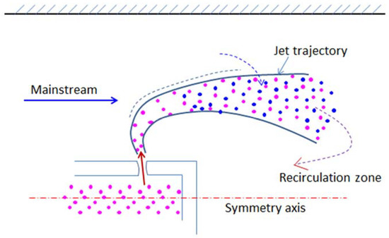
Figure 1.
Schematic of a circular transverse jet in crossflow.
In this paper, numerical simulation is used to study the flow field and aerodynamic characteristics of the circular transverse jet. In order to ensure that the calculation results with high accuracy are obtained, this paper first uses different turbulence models to perform numerical calculations based on the experimental data in reference [18], and compares the calculated results with the experimental results to select the most suitable turbulence model for calculation of circular transverse jet. Then, the model is used to study the flow field structure and aerodynamic characteristics of the circular transverse jet in crossflow.
2. Turbulence Model Selection and Analysis
In order to save the research cost and speed up the research, most scholars currently use numerical simulation to study the flow field of the transverse jet: Qiu used the k-ε standard model for numerical simulation of flowing residence characteristics of the transverse jet [19]; Song and Zhang conducted numerical simulation research on turbulent drag reduction characteristics of transverse jets, using the turbulence model SST k-ω [20]; Demena used the RSM turbulence model to analyze the flow field of the transverse jet in crossflow [21]. However, from the open literature, there is no report on the selection of a suitable turbulence model used for the numerical simulation of the transverse jet, and no unified conclusion has been formed.
Since the turbulence model has a great influence on the simulation results, especially for complicated shear flow and vortex. It is necessary to fundamentally analyze and compare the turbulence models, and select the most suitable turbulence model for the numerical simulation of the circular transverse jet to ensure the accuracy and effectiveness of the research.
This paper theoretically analyzes four turbulence models, k-ε standard, k-ε Realizable, SST k-ω, and RSM (linear pressure–strain), which are used to solve the N–S equation (RANS) by the Reynolds average method. Then, the four turbulence models are used to numerically simulate the cold flow field of the circular transverse jet in crossflow, and the obtained jet trajectory is compared with the test results to select the most suitable turbulence model.
2.1. Theoretical Analysis of Turbulence Models
For the numerical calculation method to study the characteristics of flow, the Reynolds average method is mainly used to solve the time-averaged N–S equation (RANS), and all the turbulent scales are simulated to obtain the average flow field characteristics. In order to make the N–S equation closed, there are two kinds of the RANS model that can be used: the eddy viscosity model based on the Boussinesq hypothesis and the Reynolds stress model (RSM) based on the Reynolds stress transport equation. Among them, the eddy viscosity model connects the Reynolds stress and the average velocity gradient through Boussinesq hypothesis to make the equations closed. The advantage of this hypothesis is that it only needs a very low calculation cost to calculate the turbulent viscosity [22]. Under this assumption, the k-ε model based on the turbulent kinetic energy k, the turbulent dissipation rate ε, and the k-ω model based on the turbulent kinetic energy k, the specific dissipation rate ω were developed. The RSM model uses the transport equation directly to solve the Reynolds stress, which avoids the viscosity assumption like in other models, but takes up more CPU time and memory.
In this paper, four turbulence models, k-ε standard, k-ε Realizable, SST k-ω, and RSM, which are commonly used in complex flows and are most frequently used in various studies in the literature, are studied in the numerical simulation. The comparison of their transport equations and applicable ranges is shown in Table 1. In Table 1, t is time, x and y are coordinate axes, ρ is the fluid density, μ is the fluid viscosity, μt is the turbulent viscosity, ν is the dynamic viscosity, ui is the velocity component in the i direction, and Gk represents the generation of turbulence kinetic energy due to the mean velocity gradients, Gb is the generation of turbulence kinetic energy due to buoyancy, Gω represents the generation of ω, YM represents the contribution of the fluctuating dilatation in compressible turbulence to the overall dissipation rate, Yk and Yω represent the dissipation of k and ω due to turbulence, σk and σε are the turbulent Prandtl numbers for k and ω, respectively, Γk and Γω represent the effective diffusivity of k and ω, Dω represents the cross-diffusion term, C1ε, C2, C2ε, and C3ε are constants, Rε is an additional term in the ε equation, and Sk and Sε are user-defined source terms.

Table 1.
Comparison of four different turbulence models.
2.2. Modeling and Grid Generation
The combustor model is simplified as a cylindrical tube with a length of 500 mm and a diameter of 200 mm. A nozzle pipe with a gap jet is coaxially arranged in the center of the tube. The tube and the nozzle pipe are shown in Figure 2. A small circular gap is designed on the circular wall of the nozzle pipe head. Through the nozzle jet, air, oil, and gas mixture or gaseous fuel can be injected into the mainstream. The diameter of the nozzle pipe is 20 mm, the length is 200 mm, and the gap width is 1.12 mm.
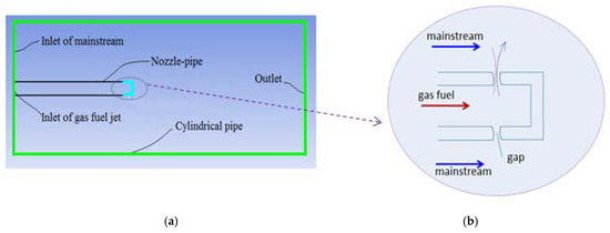
Figure 2.
Schematic of the calculation model. (a) The whole schematic of the calculation model; (b) Enlarged view of the nozzle pipe jet.
Since the gap that the fuel jet goes through is small, the influence of the near-wall boundary layer needs to be well resolved in meshing. In some turbulence models, the near-wall function must be used. The enhanced wall treatment is used to calculate the gap flow, and the thickness of the first layer near-wall grid is 0.0014 mm to make sure y+ ≈ 1. For the purpose of an optimal time consumption while ensuring simulation accuracy, the entire flow area is divided into several parts while meshing the model. The grid is refined in the vicinity of the jet injection area and the recirculation area, while in other areas the grid can be thicker. The solver fluent is used, and axisymmetric two-dimensional numerical simulations were carried out. In order to evaluate the mesh independence, the grids with numbers of 59,600, 119,200, and 171,000 were independently verified. When the grid number exceeded 119,200, the calculated results of the backflow recirculation boundary agreed with each other. Therefore, a grid with a cell number of 119,200 is selected in current simulations.
According to the results of experiments, Kosterin [18] found that the aerodynamic parameter-momentum ratio q = (ρjυj2)/(ρ0υ02) is a similar parameter for the flow of the circular transverse jet in crossflow, where , are the density and velocity of jet gas, respectively, represent the density and velocity of the mainstream. When q = const, the sizes and parameters of the recirculation zone, the circulation zone, and the jet trajectory do not change with the parameters of the mainstream and the jet. In the numerical simulation, the momentum ratio q = (ρjυj2)/(ρ0υ02) = 30, which is consistent with the experimental data (in order to ensure the similarity between the numerical simulation and the test, the same momentum ratio shall be taken for comparison).
In order to avoid the introduction of different combustion models to produce multiple variable factors, this paper only studies the nonreactive flow characteristics behind the aerodynamic flame stabilizer so as to select the appropriate turbulence model. Therefore, only air is used in the mainstream and jet components. When q = 30, the mainstream inlet flow rate is 1.39 kg/s, the total temperature is 488 K, the pressure is 1 atm, and its component is air; the gap jet inlet flow rate is 0.019 kg/s, the total temperature and the pressure are the same as mainstream, and its component is also air.
When the number of iterations reaches 10,000, the residuals of continuity, k, ε are smaller than 1 × 10⁻⁵, the residuals of x-velocity, y-velocity, and swirl are close to 1 × 10⁻⁶, the residual of energy is smaller than 1 × 10⁻⁷, and all these residuals approximately stay constants, as shown in Figure 3, it can be thought that the calculation is converged.
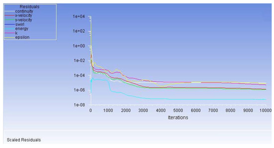
Figure 3.
Scaled residuals of iterations.
2.3. Numerical Simulation Results and Comparison with Experimental Data
2.3.1. Comparison of Velocity Field Distribution under Four Turbulence Models
According to the numerical simulation results, velocity contours under different turbulence models can be obtained as shown in Figure 4.
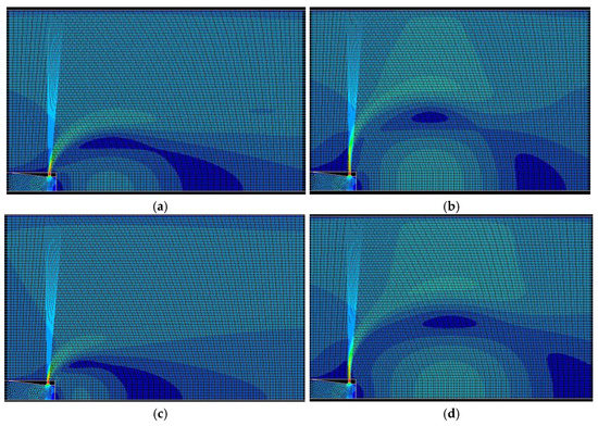
Figure 4.
Velocity contours calculated under different turbulence models. (a) k-ε standard; (b) k-ε Realizable; (c) SST k-ω; (d) RSM—linear pressure–strain.
Taking the jet nozzle pipe size as a reference, it is obvious that there are differences in the velocity field distribution under each turbulence model, and from the velocity field distribution, it can be qualitatively determined that k-ε Realizable and RSM turbulence models calculate the largest recirculation zone, but under the k-ε standard turbulence model, the recirculation zone is the smallest.
A section 40 mm downstream from the center point of the nozzle pipe end is selected, and the velocity profiles on the section under four different turbulence models are obtained as shown in Figure 5.
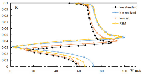
Figure 5.
Velocity profiles of the section 40 mm from the center point of the pipe nozzle end under different turbulence models.
It can be seen from Figure 5 that the velocity profiles calculated by the four turbulence models are different: the points with maximum velocity obtained by the k-ε Realizable and RSM models are farthest from the central symmetric axis, while the points with maximum velocity obtained by the k-ε standard are closest to the central symmetric axis; the backflow velocity calculated by the k-ε standard model on the central symmetric axis is the smallest, and the result calculated by the k-ε Realizable model is the largest.
2.3.2. Jet Trajectories under Four Turbulence Models and Comparison with Experimental Results
In order to accurately and quantitatively compare with the test results, it is necessary to obtain the jet trajectory, which is a curved surface formed by the maximum velocity point on each cross-section after the interaction of the jet with the mainstream. In the numerical simulation, selecting several sections and getting the coordinates of the maximum velocity points on each section, the connection of the coordinates of the maximum velocity points constitutes the jet trajectory. In order to make the calculation results dimensionless, the coordinates of each point are transformed into x/(b0d0)0.5 and y/(b0d0)0.5 coordinate systems (b0—the gap width, d0—the nozzle pipe diameter), and the jet trajectory in this coordinate system is obtained. The jet trajectory under each turbulence model and test data [18] are shown in Figure 6.
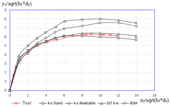
Figure 6.
Jet trajectory calculated under different turbulence models and the results of the experiment ().
It can be seen from Figure 6 that the overall shape of the jet trajectory under the four turbulence models is similar to a part of the ellipse, and the jet trajectory width increases gradually along the main flow direction, but reaches the maximum value to a certain extent, and then the jet trajectory begins to shift downward to the direction of the axis under the influence of the reverse flow in the recirculation zone. However, from the dimension of jet trajectory, the calculation results of the four turbulence models are different. The calculation results of the turbulence model k-ε Realizable and RSM greatly deviate from the experimental results, and the calculation results of the k-ε standard and SST k-ω turbulence models are relatively close to the experimental results.
The maximum width xmax and the corresponding axial position ymax at the maximum width of the jet trajectory under each turbulence model and the corresponding experimental results [18] in the x/(b0d0)0.5 and y/(b0d0)0.5 coordinate systems are shown in Table 2.
Table 2.
The maximum width of jet trajectory and the corresponding position in the coordinate system x/(b0d0)0.5 and y/(b0d0)0.5 under different turbulence models ().
As can be seen from Table 2:
- For xmax, the result of calculation by the k-ε Realizable model is the largest, by RSM model is the second, and by the k-ε standard model is the smallest; for ymax, the results of calculation by RSM model is the largest, by the k-ε Realizable model is the second, and by the k-ε standard model is the smallest.
- The results of calculation by the k-ε Realizable and RSM are both larger than the experimental values. The calculation results of the SST k-ω turbulence model are closest to the experimental values. The results of the k-ε standard model are smaller than the experimental values. The deviations of xmax and ymax under the k-ε standard model are 4% and 11.1%, respectively. The results of the SST k-ω turbulence model are close to the experimental values. The relative deviations of and ymax calculated by the SST k-ω turbulence model are 1.3% and 0% to the experimental values, respectively. While the relative deviations of xmax and ymax calculated by the k-ε Realizable model are 27.0% and 11.1%, the relative deviations of xmax and ymax calculated by the RSM linear pressure–strain model are 20.6% and 33.3%. It can be seen that when q = 30, the calculation results of the turbulence model SST k-ω are in the best agreement with the experimental results.
From the simulations above, the following conclusion can be obtained.
The jet trajectory size obtained by the k-ε Realizable or RSM turbulence models is larger than the experimental value and the deviation value is big. The jet trajectory size obtained by the k-ε standard turbulence model is smaller than the experimental value, and the calculation results under SST k-ω turbulence model best agree with the experimental results.
3. Flow Structure and Aerodynamic Characteristics
3.1. Research on Flow Field Structure
Using the turbulence model SST k-ω obtained in Section 2, the flow field structure and flow characteristics of the circular transverse jet in crossflow are studied in detail. The velocity contours are shown in Figure 7. From Figure 7, it can be seen that the jet bends downstream in the crossflow, and forms an obvious dome-shaped aerodynamic barrier composed of high-speed jet trajectory. Behind this aerodynamic barrier, several low-velocity zones are formed, as shown by the dark blue area in Figure 7. From the two-dimensional figure, there are three low-speed zones behind the aerodynamic barrier, but reflected in the actual three-dimensional structure, the symmetrical low-speed zones directly under the jet trajectory are a continuous circular low-speed zone, and near the axis of symmetry behind the circular low-speed zone there is a tail low-velocity zone with a large projection area.
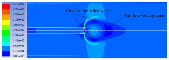
Figure 7.
Velocity contours of the flow field at .
The static pressure distribution in the flow field is shown in Figure 8. It can be seen from Figure 8 that there is an axial symmetric negative pressure area behind the jet trajectory, and the lowest negative pressure value relative to the crossflow, in this case, is −7460 Pa.
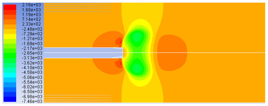
Figure 8.
Static pressure contours of the flow field at q = 30.
The velocity vector diagram of the flow field is shown in Figure 9. It can be seen from Figure 9 that an obvious recirculation zone is formed behind the jet trajectory, and the recirculation zone is composed of a pair of the axial symmetric vortex on the two-dimensional projection. The pair of the axial symmetric vortex is a vortex ring in the three-dimensional actual structure. According to the velocity vector diagram in Figure 9, the flow mechanism under the interaction of the jet with crossflow can be analyzed as follows: under the barrier effect of the high-speed jet, an axial symmetric negative pressure zone is formed behind the jet. Because of the pressure gradient, the surrounding fluid is sucked into the negative pressure zone, and forms a reverse flow axial velocity of which is opposite to the crossflow. The reverse flow flows until contact and mixes with the newly ejected jet flows downstream. Zone A in Figure 9 represents the center area of the vortex, which corresponds to the circular low-velocity zone in Figure 8, and Zone B borders the reverse flow and the forward flow, and corresponds to the tail low-velocity zone in Figure 7. Region C is the region with the fastest reverse flow velocity after the reverse flow is accelerated by the negative pressure zone, and then the reverse flow velocity decreases due to the blocking effect of the jet.
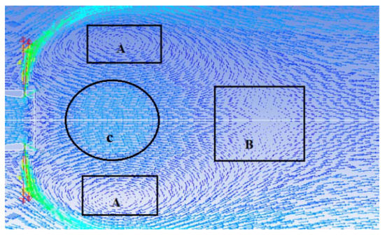
Figure 9.
Velocity vectors colored by velocity magnitude of the flow field at .
The enlarged view of the vortex center in Zone A in Figure 9 is shown in Figure 10. It can be seen that the vortex center is a recirculation flow, and the velocity of the center part is smaller than that of the periphery part.
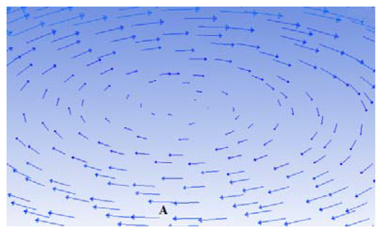
Figure 10.
Velocity vectors colored by velocity magnitude in Zone A.
Obtain the pathlines diagram of the flow field, as shown in Figure 11. The figure shows the fluid flow process in the recirculation zone very visually. In addition to the obvious symmetrical vortex structure and the structure of the recirculation zone, it can also be seen from Figure 11 that in front of the jet, there is a pair of ear-shaped small-sized axial symmetric vortex structures along the wall of the jet device. The vortex is formed under the blocking of crossflow by the high-speed jet and the interaction with the boundary layer of the wall.
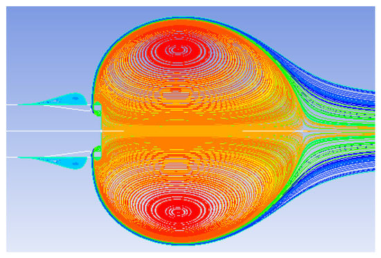
Figure 11.
Pathlines around the recirculation zone of the flow field at .
3.2. Research on Flow Field Characteristics
According to the definition of the recirculation zone, the boundary of the recirculation zone can be obtained by the isosurface of the axial flow velocity equal 0, as shown in Figure 12.
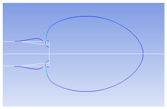
Figure 12.
Boundary of recirculation zone at .
It can be seen from Figure 12 that the boundary of the recirculation zone is similar to an ellipse in shape. Taking several points on the boundary of the recirculation zone to measure the size of the recirculation zone, taking the center point of the jet exit from the jet device as the coordinate origin and converting them to the dimensionless coordinate system x/(b0d0)0.5 and y/(b0d0)0.5, the recirculation zone size can be obtained as shown in Figure 13. Due to axial symmetry, the boundary of the recirculation zone is only half drawn.
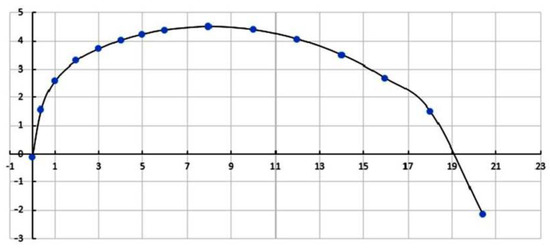
Figure 13.
Size of recirculation zone at q = 30.
Considering the length/width ratio can describe the shape of the ellipsoid. According to Figure 13, the length/width ratio of the recirculation zone, in this case, can be calculated as 1.52.
In order to study the length/width ratio of the recirculation zone under different working conditions, several cases were calculated at different momentum ratios (ρjυj2)/(ρ0υ02), which is considered to be the similarity parameter of jet flow. By regulating the flow rates of the circular transverse jet, the sizes of the recirculation zone were obtained and presented in Table 3.
Table 3.
Dimensions of recirculation zone under different boundary conditions.
The relationship between the length/width ratio and momentum ratio is shown in Figure 14.
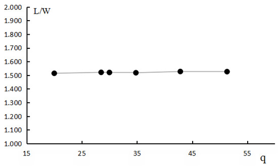
Figure 14.
Length/width ratio with different momentum ratio q.
It can be seen from Figure 14 that the length to width ratio L/W is basically constant, independent of the momentum ratios (ρjυj2)/(ρ0υ02). It means that the shape of the recirculation zone does not change with the parameters of crossflow and circular transverse jet when the geometry parameters of the jet device do not change.
4. Conclusions
After the above numerical calculations, the following conclusions can be obtained:
- For the circular transverse jet, the numerical results calculated by the SST k-ω model is best consistent with the experimental results. Turbulence model SST k-ω is the best suitable model for the numerical simulation of the circular transverse jet among these four calculated turbulence models (k-ε standard, k-ε Realizable, SST k-ω, and RSM).
- In the flow field, under the interaction of the circular transverse jet with the crossflow, an axial symmetric negative pressure zone is formed behind the jet trajectory, and there exists an axial symmetric vortex structure due to the sucking effect of the negative pressure zone. This structure causes the reverse flow of the fluid behind the jet trajectory, forming a typical recirculation zone. Since the existence of the recirculation zone playing an important role in flame stabilization, the circular transverse jet would be a potential method for the stable combustion system.
- Through the comparison of multiple groups of numerical results, it is found that the recirculation zone formed by the interaction of the circular transverse jet with crossflow has a constant length/width ratio. It means that the shape of the recirculation zone is not affected by the crossflow and jet parameters under the condition of unchanging geometric sizes of jet devices.
The work in this paper would be a fundamental reference for the study of fuel/air mixing characteristics and combustion efficiency in the flow field formed by circular transverse jet in crossflow in future.
Author Contributions
Investigation and writing, Z.L. and Y.Y., review and editing, V.L.V., B.G., and J.Y. All authors have read and agreed to the published version of the manuscript.
Funding
This research was supported by National Key Research and Development Program of China (No. 2016YFC0802704), National Natural Science Foundation of China (No.50876104), and Chinese-Russian cooperation and exchange project of the Chinese Academy of Sciences (Y9290382W1).
Acknowledgments
The present work is an extension of the paper FMIA811 of the 4th International Conference on Fluid Mechanics and Industrial Applications. The authors are grateful to the National Natural Science Foundation of China, National Key Research and Development Program of China, and the Chinese-Russian cooperation and exchange project of the Chinese Academy of Sciences.
Conflicts of Interest
We declare that there are no conflict of interest.
References
- Nair, V.; Wilde, B.; Emerson, B.; Lieuwen, T. Shear Layer Dynamics in a Reacting Jet in Crossflow. Proc. Combust. Inst. 2019, 37, 5173–5180. [Google Scholar] [CrossRef]
- Panda, P.P.; Busari, O.; Roa, M.; Lucht, R.P. Flame stabilization mechanism in reacting jets in swirling vitiated crossflow. Combust. Flame 2019, 207, 302–313. [Google Scholar] [CrossRef]
- Huang, R.F.; Kimilu, R.K.; Hsu, C.M. Effects of jet pulsation intensity on a wake-stabilized non-premixed jet flame in crossflow. Exp. Therm. Fluid Sci. 2016, 78, 153–166. [Google Scholar] [CrossRef]
- Smith, S.H.; Mungal, M.G. Mixing, structure and scaling of the jet in crossflow. J. Fluid Mech. 1998, 357, 83–122. [Google Scholar] [CrossRef]
- Moussa, Z.M.; Trischka, J.W.; Eskinazi, S. The nearfield in the mixing of a round jet with a cross-stream. J. Fluid Mech. 1977, 80, 49–80. [Google Scholar] [CrossRef]
- Karagozian, A.R. Transverse jets and their control. Prog. Energy Combust. Sci. 2010, 36, 531–553. [Google Scholar] [CrossRef]
- Wagner, J.A.; Grib, S.W.; Renfro, M.W.; Cetegen, B.M. Flowfield measurements and flame stabilization of a premixed reacting jet in vitiated crossflow. Combust. Flame 2015, 162, 3711–3727. [Google Scholar] [CrossRef]
- Rugger, R.; Callaghan, E.; Bowden, D. Penetration of air jets issuing from circular, square and elliptic orifices directly perpendicularly to an air stream. NACA TN. 2019. Available online: http://naca.central.cranfield.ac.uk/report.php?NID=4008 (accessed on 9 June 2020).
- Keffer, J.; Baines, W.D. The round turbulent jet in a cross-wind. J. Fluid Mech. 1962, 15, 481–496. [Google Scholar] [CrossRef]
- Kamotani, Y.; Greber, I. Experiments on a turbulent jet in a cross flow. AIAA J. 1972, 10, 1425–1429. [Google Scholar] [CrossRef]
- Fric, T.F.; Roshko, A. Vortical structure in the wake of a transverse jet. J. Fluid Mech. 1994, 279, 1–47. [Google Scholar] [CrossRef]
- Kelso, R.M.; Lim, T.T.; Perry, A.E. An experimental study of round jets in cross-flow. J. Fluid Mech. 1996, 306, 111–144. [Google Scholar] [CrossRef]
- Yuan, L.L.; Street, R.L. Trajectory and entrainment of a round jet in crossflow. Phys. Fluids 1998, 10, 2323–2335. [Google Scholar] [CrossRef]
- Cortelezzi, L.; Karagozian, A.R. On the formation of the counter-rotating vortex pair in transverse jets. J. Fluid Mech. 2001, 446, 347–373. [Google Scholar] [CrossRef]
- Muppidi, S.; Mahesh, K. Direct numerical simulation of round turbulent jets in crossflow. J. Fluid Mech. 2007, 574, 59–84. [Google Scholar] [CrossRef]
- Huang, R.F.; Hsieh, R.H. Sectional flow structures in near wake of elevated jets in crossflow. AIAA J. 2003, 41, 1490–1499. [Google Scholar] [CrossRef]
- Kosterin, V.A.; Rogozhin, B.A.; Dudkin, V.T. Calculation of a combustion chamber with flame stabilizers. Burn. Stream 1970, 141–159. [Google Scholar]
- Lebedev, B.P.; Kosterin, V.A.; Gordon, M.S.; Zikeev, V.S.; Nosov, L.A. Aerodynamic Stabilization of Flame in Afterburners; Proceedings of CIAM: Moscow, Russia, 1977. [Google Scholar]
- Qiu, H.; Zhang, J.; Sun, X.; Chang, J.; Bao, W.; Zhang, S. Flowing residence characteristics in a dual-mode scramjet combustor equipped with strut flame holder. Aerosp. Sci. Technol. 2020, 99, 105718. [Google Scholar] [CrossRef]
- Song, X.; Zhang, M. Turbulent Drag Reduction Characteristics of Bionic Nonsmooth Surfaces with Jets. Appl. Sci. 2019, 9, 5070. [Google Scholar] [CrossRef]
- Demena, A.M. Development of Methodological Foundations of Gas-Dynamic Flame Stabilization for Combustion Chambers on Swirling High-Enthalpy Jets. 2008. Available online: https://www.dissercat.com/content/razrabotka-metodicheskikh-osnov-gazodinamicheskoi-stabilizatsii-fronta-plameni-potochnykh-ka (accessed on 9 June 2020).
- Zhao, F.; Zhang, Y.; Zhu, R.; Wang, H. Turbulence model in supersonic jet flow field. J. Univ. Sci. Technol. Beijing 2014, 36, 366–371. [Google Scholar]


© 2020 by the authors. Licensee MDPI, Basel, Switzerland. This article is an open access article distributed under the terms and conditions of the Creative Commons Attribution (CC BY) license (http://creativecommons.org/licenses/by/4.0/).