All articles published by MDPI are made immediately available worldwide under an open access license. No special
permission is required to reuse all or part of the article published by MDPI, including figures and tables. For
articles published under an open access Creative Common CC BY license, any part of the article may be reused without
permission provided that the original article is clearly cited. For more information, please refer to
https://www.mdpi.com/openaccess.
Feature papers represent the most advanced research with significant potential for high impact in the field. A Feature
Paper should be a substantial original Article that involves several techniques or approaches, provides an outlook for
future research directions and describes possible research applications.
Feature papers are submitted upon individual invitation or recommendation by the scientific editors and must receive
positive feedback from the reviewers.
Editor’s Choice articles are based on recommendations by the scientific editors of MDPI journals from around the world.
Editors select a small number of articles recently published in the journal that they believe will be particularly
interesting to readers, or important in the respective research area. The aim is to provide a snapshot of some of the
most exciting work published in the various research areas of the journal.
The energy interaction among a load service entity and community energy systems in neighboring communities leads to a complex energy generation, storage, and transaction problem. A load service entity is formed by a local electricity generation system, storage system, and renewable energy resources, which can provide ancillary services to customers and the utility grid. This paper proposes two coordination schemes for the interaction of community-based energy systems and load service entities based on game-theoretic frameworks. The first one is a centralized coordination scheme with full cooperation, in which the load service entity and community energy systems jointly activate the local resources. The second one is set as a decentralized coordination scheme to obtain a relative balance of interests among the market participants in a Stackelberg framework. Two mathematical models are developed for the day-ahead decision-making of the above energy management schemes. The Shapley value method, Karush-Kuhn-Tucker conditions, and strong dual theory are applied to solve the complex coordination problems. Numerical study shows the effectiveness of the coordination strategies that all stakeholders benefit from the proposed coordination schemes and create a win–win situation. In addition, sensitivity analysis is conducted to study the effects of system configuration, energy demand, and energy prices on the economic performance of all stakeholders. The results can serve as references for business managers of the load service entity.
The energy crisis has attracted significant attention in recent years. As the basic social unit, communities may significantly affect the energy utilization of humans. In local communities, the energy system is undergoing a revolution towards a more environmentally sustainable and renewable, energy-based system [1]. Community energy systems (CES) are attracting more and more attention while facing a paradigm shift in the energy sector [2]. The CES is an efficient system to coordinate the distributed energy resources and reorganize the local energy systems [3]. The advantages of energy utilization improvement, carbon emission reduction, and reliability enhancement can be achieved by the CES, which is not only to satisfy the energy demand of communities but also to implement energy exchange with other subjects [4]. The CES can couple electricity, heating, and cooling sectors with generation and storage devices like photovoltaic (PV) wind turbines, gas-fired combined heat and power systems (CHP), heat pumps, boilers, chillers, energy storage, etc. It has been proven that the CES can offer multiple benefits and will play an important part in future energy systems, providing energy with lower annual cost and lower carbon emissions compared with the conventional energy systems. A load service entity (LSE) is formed by local electricity generation systems, storage systems, and renewable energy resources to increase the elasticity of demand management and offer a certain degree of flexibility in its energy exchange [5]. A LSE can provide ancillary services to customers and the utility grid, such as provide an incentive price to customers with a set of schedulable assets to encourage them participating in the local market, and provide upward/downward power to compensate the imbalances in the regulated power market [5,6]. Therefore, the LSE is a key component in the energy system as it is a medium that connects the retail market and wholesale market. Moreover, the LSE can exchange electricity bilaterally with the local CESs. The LSE may possess distributed energy resources and can also trade electricity with privately-owned energy systems (e.g., third party companies, households) [7]. If the LSE buys electricity from privately owned energy systems, it should pay these entities for the electricity. The goal of a LSE is to maximize its profits, which contains the operation cost and the electricity transaction cost/profit with the utility grid and CESs. Hence, it is necessary to explore how to facilitate energy interaction effectively between selfish individual CESs in a local area, and how to coordinate the LSE and CES operation strategies for obtaining a relative balance of interests among the market participants. Therefore, the coordinated energy management scheme should be developed.
Several studies have been conducted on the energy management of CESs according to game theory approach. On one hand, in order to maximize the utilization of local resources, the cooperation of stakeholders is an effective way for maximizing social welfare [8]. In Reference [9], the operation management of multiple energy systems has been explored based on the maximum of overall economic benefits. The profit allocation strategy among the distributed energy network participants is formed based on the core method of cooperative game theory. In Reference [10], a cooperative game-theoretic analysis is applied for the microgrids cooperation in regulated electricity markets. How the microgrid affects costs and benefits for all parties is quantified. In Reference [11], cooperative game theory is applied to construct an energy grand coalition for minimizing the coalitional energy cost. It is demonstrated that energy coalitions are effective to reduce the variability of a local network load profile. In Reference [12], a group of individual multi-microgrids coordinating problem is solved by a cooperative game approach considering the network losses. A cost allocation method based on the concept of core is implemented. In summary, the cooperative game theory, which could guarantee a global operation economy efficiently, has proved its success to address the conflict of interests in the local energy system. However, the coordination and profit/cost allocation between load service entity and community energy systems with electricity and heat under a cooperative game framework is paid little attention. Thus, the coordination strategy between the LSE and CESs is explored based on a cooperative game framework in this paper.
On the other hand, the hierarchical framework is utilized to address the coordination problem among stakeholders using a decentralized model. Such a hierarchical structure can be backward in leader-follower type (Stackelberg game) models, under the assumption that the leaders can anticipate the rational reaction of followers [13]. In Reference [14], an electricity control strategy for the coordinated operation of a distribution network operator and microgrids is proposed. The distribution network operator is at the upper level and the microgrids are at the lower level, and they are considered as entities with individual objectives to minimize their operation costs. In Reference [15], a multi-follower bi-level programming is built to optimize the interaction between the distribution networks and autonomous microgrids considering the demand response. Reference [16] forms a hierarchical decision-making framework to decide the electricity trading price between a distribution company and microgrids. Another price decision approach in a hierarchical energy system is assumed as a linear relationship between the electricity price and aggregated demand [17]. These recent studies mainly focused on the electricity interactions between the distribution networks and microgrids in a hierarchical framework, and few studies have concentrated on the distributed interaction between load service entities and multiple multi-energy-community energy systems using a game theory approach. If multiple energy demands are covered in community energy systems, the optimal scheduling of the community energy system is more complex than full electric microgrids. Reference [5] presents a price decision method for load service entities and microgrids. A genetic algorithm is applied to search the best trading price for each microgrid and the load service entity. The fitness function of the genetic algorithm is the total cost of the load service entity and microgrids. Due to the characteristic of the genetic algorithm, a local best solution may emerge, and the interest of each stakeholder cannot be guaranteed. In this paper, the coordination strategy between the LSE and CESs is optimized using a bilevel approach under a Stackelberg framework, based on a proposed pricing strategy, to make the CESs have enough motivation to cooperate with the scheduling of LSE and balance the operational cost of each participant.
Decision models in a hierarchical structure are frequently modeled as bilevel problems [18]. All the participators pursue their own maximum profits. In this case, the leads in the upper level problem incorporate their optimization problems with the rational reaction functions of the followers. The closed form expression of the latter is obtained by solving the followers’ optimization problems of the Stackelberg game first, considering as fixed the variables of the leaders. Then, the leaders incorporate the followers’ reaction functions in their optimization problems, therefore proceeding backward. For solving the bilevel problems, Karush-Kuhn-Tucker (KKT) conditions can be introduced and the problem is reformed into a single-level problem with equilibrium constraints. The conversion strategy is usually used in strategic decision making [19], contract price optimization [20], and other problems.
Based on the above-mentioned literature review, there are some gaps that need to be fulfilled. The coordination and profit allocation between the load service entity and community energy systems with flexible electricity and heat demand under a cooperative game framework is paid little attention. Besides, under a Stackelberg framework, little literature focused on the coordination between the LSE and CESs based on a pricing strategy, which can make the CESs having enough motivation to cooperate with the scheduling of LSE and balance the operational cost of each participant. Therefore, to coordinate the operation strategies of LSE and CESs for obtaining a relative balance of interests among the market participants, and to facilitate energy interaction effectively in a local area, the coordinated energy management schemes should be explored while facing a significant increase in CESs. In this paper, two coordination schemes based on the Cooperative game and Stackelberg game theory are proposed to optimize the interactive strategies of LSE and CESs. The centralized coordination scheme is focused on the maximum social welfare of the whole area, while considering individual and group incentives, as well as various fairness properties. The decentralized coordination scheme is developed to minimize selfish individual costs of all local market participators, and to obtain a relative balance of interests among the market participants in a regulated environment. Then, the two schemes are thoroughly compared and analyzed.
The contributions are as follows:
A centralized coordination scheme for the interaction among the LSE and CESs is proposed. A local energy coalition among entities under a centralized control is formed to minimize the joint coalitional energy cost based on cooperative game theory. A cost-sharing scheme is developed according to the Shapley value method, which ensures that all stakeholders are financially rewarded, and discourages stakeholders deviating from the expected cooperation.
A decentralized coordination scheme is developed to coordinate the LSE and CESs sequentially. A bilevel programming model is proposed to optimize the day-ahead interactive strategies between the LSE and CESs that providing insight on LSE-CESs coordination under a Stackelberg framework. A win-win situation is established in a decision-making process in which the interests of LSE and each CES are considered simultaneously according to a pricing strategy of electricity.
Sensitivity analysis is conducted to investigate the effects of system configuration, energy demand, and energy market prices on the economic performance of all stakeholders under the centralized coordination scheme and decentralized coordination scheme.
2. Problem Description
In an area, a LSE and several independent CESs exist. The relationship between the LSE and CESs is shown in Figure 1. Blue and red lines indicate electricity and heat flow. The CESs dispose of a set of generation assets that are comprised of natural gas fired equipment, generation equipment of renewable energy, energy storage, and so on. Electricity can be bought and sold among utility grid, LSE, and CESs. The LSE can provide ancillary services to the utility grid and an incentive price to consumers [6]. It is assumed that minimizing the cost or maximizing self-interest is the first priority for all actors. To increase the social welfare of the area and support the LSE operation strategy in considering the interactions with CESs, the decision-making process needs to be thoroughly analyzed.
2.1. Load Service Entity
The LSE contains PVs and an electrical storage. The model of LSE can be described as follows:
subject to
Equation (1) is the objective function of the LSE. Equations (2)–(3) represent the electricity flow constraints. The cost of the LSE in Equation (1) contains the costs of the electricity interaction between the LSE and CESs, electricity trading between the LSE and utility grid, and the O&M (Operation and Maintenance) costs of the PVs and electrical storage. Equation (2) shows the electricity balance during each period. To avoid buying and selling power from and to the utility grid simultaneously, Equation (3) is considered. The constraints for PV and electric storage equipped by the LSE are Equations (4)–(9). In this paper, the limits of power networks are assumed to be adequately large for distributing power without causing congestion. This assumption is also made in the References [21,22,23].
If the LSE has the authority to decide the internal trading prices while coordinating with the CESs, Equations (10)–(12) are listed to represent the LSE operation constraints in a regulated environment.
To avoid CESs against high-energy prices, Equation (10) is set for limiting the market power of LSE and constraining total expenditure of CES transacted with LSE, which should be no more than that of CES traded with the energy market directly [24]. Factor is slightly smaller than one and can be used to change the costs of the LSE and CESs to form a win-win situation. To avoid “response fatigue” due to price variation, the hourly price variations are limited in Equation (11) [25]. The upper and lower bounds of hourly interaction prices are set in Equation (12) to keep the interaction stable.
2.2. Community Energy System
Each CES may contain various equipment. The electrical demand can be met by a combined heat and power system, photovoltaic, etc. A CHP system, gas fired boiler, thermal storage etc. can supply heat to satisfy the thermal demand. In addition, the CES operators could not only manage the generation and storage equipment, but also manage their elastic loads based on the framework of demand response. The model of CES q is built as follows.
subject to
Equation (13) is the objective function of the CES. Equations (14)–(15) represent the energy flow constraints, and Equations (16)–(20) capture the CES operation constraints. The objective of the CES problem is to minimize the overall cost in Equation (13), which contains the interaction costs with the LSE and utility grid, operation cost of the CES and cost of electricity demand response. From the point of view of applicability and economy in the city area, four types of equipment are considered in the CES: CHP, boiler, PV, and heat storage, which represent the gas fired equipment, renewable energy devices, and storage. For gas-fired equipment in the CES, the operations cost includes the natural gas cost and O&M cost. Equations (14) and (15) show that the supply of electricity and heat must be no less than the energy demand in each CES. and represent the natural gas consumption by microturbine and boiler, and and are the heat efficiencies of the power generation unit and gas fired boiler [26]. Equation (16) limits the load curtailment for CESs during each period according to the demand response contract signed by consumers. represents the amount of electrical load curtailment. It is assumed that the load demand of consumers under each CES includes two parts: inelastic load and elastic load. The inelastic load should be met exactly, and the elastic load can be curtailed [16]. Equation (17) is the upper and lower generation or storage bounds for microturbines, boilers, photovoltaics, and thermal storage. The input and output of energy storage are constrained in Equations (18)–(20) [27]. Due to the fast response speed of microturbines, the ramp rate in hourly scheduling is not considered.
3. Coordination Schemes
In this paper, two coordination schemes for the interaction between LSE and CESs, which contain a Cooperative game and a Stackelberg game, are analyzed. It is assumed that the LSE can share energy with multiple CESs, whereas two CESs do not share energy directly, because there is no overlapping between the interface nodes of two CESs. The two schemes are the centralized coordination scheme and decentralized coordination scheme, which focus on collective rationality and individual rationality.
3.1. Centralized Coordination Scheme
The centralized coordination scheme is a non-pricing-based approach, which is proposed for maximizing social welfare in an area. The participators from different interest groups coordinate together in a centralized optimization problem. To solve this problem, the following assumptions are taken into account: (1) An optimistic assumption is made that all the CESs will reveal real information to the LSE, thus, the LSE has the complete information on the energy consumption and generation preferences of each stakeholder; (2) It is assumed that if there is no LSE, each CES can only trade with the utility grid and cannot interact with other CESs. The objective function is defined as the sum of all stakeholders’ willingness-to-pay. Combining the power flow constraints of the LSE and all constraints of the CES, the Mixed-integer linear programming (MILP) model is developed as follows:
After calculating, the optimal cost of the whole energy system is achieved. The fair profit allocation plan makes stable and sustained cooperation among actors. Therefore, the cooperative game is used to explore the interaction structure within the district. In a cooperative game, the concept of core is a set of stable imputations, under which no player takes the initiative to break the coalition and no coalition can improve by changing the player’s actions [28]. Let denote the set of participators, and let coalition denote a subset of N. A payoff vector, , is related to the profit allocation strategy under a cooperative coalition. To be a coalition, the individual rationality, group rationality, and subgroup rationality must be satisfied simultaneously [9]. Thus, the following constraints are strict:
V indicates a function representing the total cost or profit. Equation (22) represents that the actor will obtain more profit in a coalition than when acting alone. In Equation (23), the sum of profits for each player should be equal to the maximum possible profit of the whole system. In addition, the overall profit earned by any formed coalitions should be no more than the allocated profit of each player, which is in Equation (24). If Equations (22)–(24) cannot be simultaneously satisfied, it can be deduced that no core is under the current imputation. The above Equations narrow down a possible range of costs or profits from the cooperation for each player.
The Core conditions described above are necessary conditions in a profit allocation scheme. Although the profit allocation plans are included in the Core, some players may view these solutions as unfair. Thus, the fairness and stability of different allocations are necessary to measure. According to References [29,30], the Fairness Index, , can be expressed as follows:
where is the Power Index, represents the standard variance, and is the average value. The lower fairness of the allocation plan is accompanied with the greater value of , and vice versa.
In addition, the concept of Propensity to Disrupt (DP) value is employed to measure the stability of a coalition based on the allocation scheme [31,32]. The DP value of player i expresses the loss of the members in coalition N except i, compared to the loss of i that refused to cooperate. The DP value, , is defined as follows:
where is the total profit of the each player except i, and is the benefit deduced by reducing player i. A player will disrupt the coalition for a high DP value. If the DP value is more than 1, the cooperation is easy to be disrupted because the loss of the members except i is larger than the loss of i if i refuses to cooperate. On the contrary, the coalition will be relatively stable if the value is less than 1, even if it becomes negative.
In this paper, the Shapley value method is used to allocate the profit gained from cooperation [33]. The marginal contribution of a player dependent on the player joining the coalition is introduced to evaluate the cost of each player. The Shapley value for player j in an n-person cooperative game, , is expressed as follows:
where is the cost or profit of coalition S, and is the value of the coalition S except player j.
3.2. Decentralized Coordination Scheme
The decentralized coordination scheme is a pricing-based approach, which is proposed for maximizing the individual profit under a hierarchical framework. In a decentralized market, the LSE is a price maker under some regulated conditions (Equations (10)–(12)), and CESs are price takers. The LSE and CESs interact in a sequential manner. The solution process can be implemented while considering the following assumptions: (1) Each stakeholder is rational and makes decisions independently to pursue its minimum cost or maximum profit; (2) to address the hierarchical structure using a Stackelberg game, it is assumed that the CESs always provide the best response to the signals of LSE, and the LSE can anticipate the rational reaction of the CES; (3) the LSE is assumed to propose prices by first anticipating the reaction of the CESs, which reacts to the signals sent by the LSE second following its reaction function. Interactive relationships among players are according to a Stackelberg game process:
The LSE proposes the day-ahead electricity trading tariffs for internal trading with the CESs. The electricity tariffs will be changed according to the decision of CESs until the LSE obtains the minimal cost.
After receiving the internal electricity trading prices, the CES decides the electricity trade amount with LSE, and its operations strategies. The CES then reports the power purchasing or selling quantity to the LSE.
The LSE adjusts its decision variables and the CESs repeatedly update their trading strategies and send feedback to the LSE.
When the Stackelberg equilibrium is obtained, any strategy changes of the players will not lead to an increase in their profits.
Herein, the LSE model contains Equations (1)–(12) and the CES model contains Equations (13)–(20). The LSE-CESs are coordinated via internal interactive tariffs. The strategic decision of each actor depends on the decisions of others, which in turn affects the decisions of others. A trade-off is formed while optimizing each objective function of the LSE and CESs. Minimizing the cost of the LSE problem requires that the LSE provide a lower selling price and a higher purchasing price for CESs, which in turn increases the trading cost of CESs and causes a decrease in the amount of interactive energy.
To address the conflicting hierarchical problem, the Karush-Kuhn-Tucker (KKT) conditions are used for the relaxation of the followers [34]. The decision-making variables in the LSE problem are considered as parameters in the CESs’ problem. The complementary constraints are nonlinear and can be linearized by the Fortuny-Amat and McCarl method [35]. Since there are too many constraints in the lower level, the KKT conditions are stated in Appendix A. The non-linear expression in Equation (1) can be replaced as a linear expression based on the strong dual theory, which is described in Appendix B. In conclusion, the bilevel problem is transformed into the mixed-integer linear problem.
Among the Equations, Equation (3) and Equations (A26)–(A42) can be linearized using Equation (A43). Then, the bilevel problem transforms into a single-level MILP.
4. Numerical Study
Three cases are designed to provide insights into how the coordination strategy affects economic performance. Case 1 is the baseline case that all stakeholders act alone with the utility grid. Case 2 considers that the LSE and CESs are in a full cooperation. The LSE and CESs under the centralized coordination scheme can exchange electricity freely. The Shapley value method is applied to allocate the profits. In Case 3, the LSE and CESs interact in a sequential manner under a Stackelberg framework. Under the decentralized coordination scheme, the internal trading price is the medium among participators. The real-time pricing scheme (RTP) is introduced.
The decision problems are solved using MATLAB & Gurobi. It is assumed that there are three CESs and one LSE in an area. Electricity trading is considered in the day-ahead problem, which is formulated within 24 h. System configurations of the LSE and CESs are shown in Table 1. The CHP unit is introduced in the CES2 and CES3. The PV and boilers are installed in all CESs. The electric storage and thermal storage are installed in LSE and CES3, respectively.
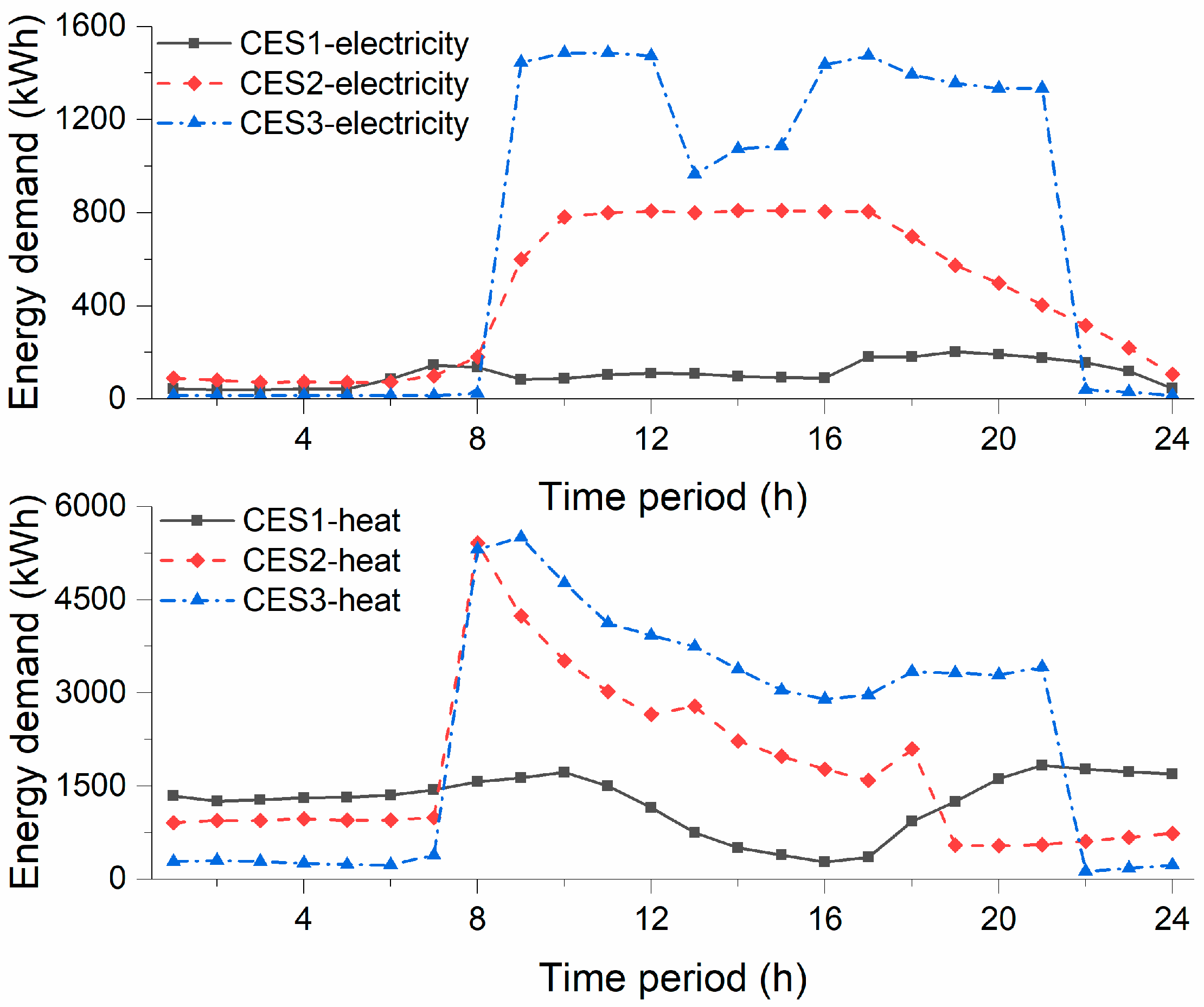
The natural gas price is $0.03/kWh. The electricity purchasing prices from the utility grid are set as time-of-use electricity prices. During periods 1–4 h and 22–24 h, the buying price was $0.06/kWh; for periods 5–7 h and 11–16 h, the price was $0.12/kWh; during periods 8–10 h and 17–21 h, the price was $0.18/kWh. The selling price to the utility grid was set at $0.05/kWh, which is the provincial benchmarking price for selling electricity to the main utility grid. The lower and upper bounds of the electricity prices between the LSE and CESs in the day-ahead trading market are set as and , respectively, which can limit the profits of the LSE. In addition, it is assumed that the demand side of CES1 can reduce the electrical load while considering the demand response program. The coefficient in Equation (10) is set to be 0.98. The distribution of energy demand in each CES is displayed in Figure 2.
5. Results and Discussion
5.1. Results
(1) Centralized coordination scheme
Four players, including one LSE and three CESs, are in the cooperative game. The set of players is N = {LSE, CES1, CES2, CES3}. The costs of 15 non-empty collections are optimized and described in Table 2.
The cost allocation strategy of the LSE and CESs are determined using the Shapley value method, as shown in Table 3.
The cost of each player should be inside the Core for any reasonable allocation scheme. According to Equations (22)–(24), it can be found that the costs after allocation satisfy the Core requirements. Therefore, the Shapley value method is feasible. Moreover, the Fairness Index and DP value in Equations (25) and (27) are calculated to measure the fairness and stability of allocation schemes. As mentioned above, the allocation scheme is in a reasonable range (0–1) of the Fairness Index. In addition, all the DP values are less than 1. It can be deduced that the current allocation scheme is feasible, fair, and stable.
(2) Decentralized coordination scheme
The Stackelberg game theory is introduced in the decentralized coordination scheme. The LSE act first to set the internal trading prices of electricity, and the CESs act as price takers following the LSE. The bilevel model is transformed into a single level MILP. The costs of the four players are in Table 4.
The optimal electricity prices are determined to activate the internal interaction among all stakeholders. In this case, purchasing and selling electricity among the LSE and CESs are allowed. The day-ahead electricity rates for CESs are evaluated over one day in Figure 3.
All the prices are relatively stable, which reduces the CESs’ risks of exposure to market volatility. The pricing strategies are strictly in accordance to the principle in Equations (10)–(12). Among the three cases, with the relative trading prices of electricity, the CES1 has the highest price. The main reason is that the CES1 is only installed with PV and most of its electricity is purchased from other CESs and LSE.
5.2. Discussion
(1) Economic assessment of the centralized and decentralized coordination schemes
The daily costs of LSE and CESs in three cases are presented in Figure 4. Negative costs can be seen as a profit. Case 1 is the basic case that all players act alone with the utility grid. Most CES programs maintain the state as this case in China. This case has the highest cost of each actor and the total cost of all actors. It can be found that the total expenditures of all stakeholders in Cases 2 and 3 decrease by 3.15% and 3.06%, respectively, when compared to the basic case. Both in Case 2 and Case 3, the cost of each stakeholder is less than the cost in the corresponding basic case. That is to say, the centralized and decentralized coordination schemes can enhance the social welfare of all stakeholders.
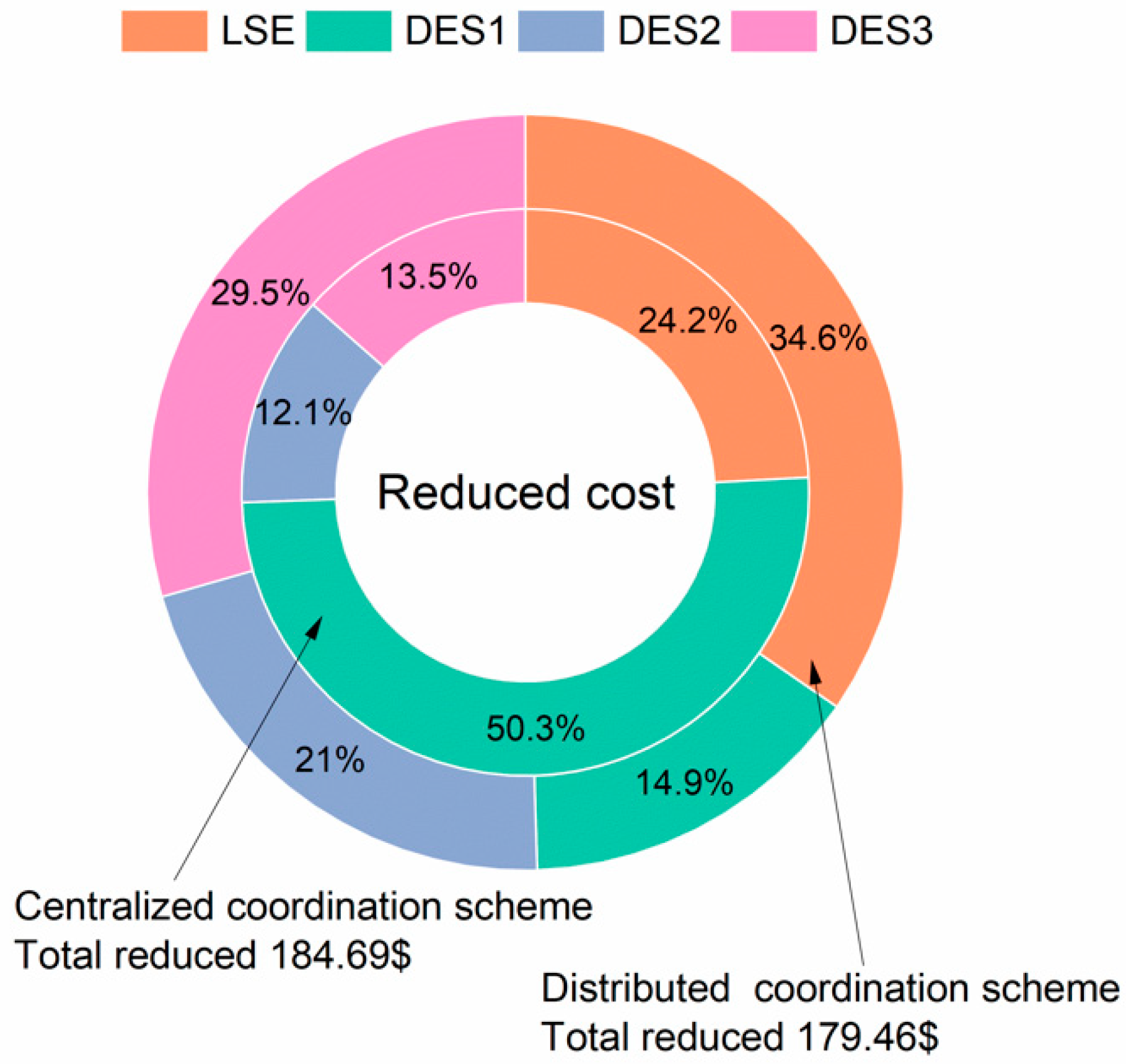
The allocation of reduced cost in Case 2 and Case 3 compared to Case 1 is shown in Figure 5. The internal circle represents the Case 2, and the external circle describes the Case 3. The total cost of all stakeholders is reduced by $184.69 and $179.46 in Case 2 and Case 3 while comparing with that in Case 1. The percentage of each actor means that the reduced cost accounts for the total reduced cost of all actors. Because of the increasing market power of LSE, it can be found that the proportion of LSE increases in the decentralized coordination case than the centralized scenario. The cost of CES1 increases along with the decrease of others’ costs. The reason is that CES1 has the lowest power generation quantity in a decentralized market and purchases lots of electricity generated by CES2 and CES3.
Obviously, compared with the decentralized coordination scheme, the centralized coordination scheme performed well from an economic point of view. The internal resources are coordinated from a total perspective, due to full cooperation. As to large-scale problems with multiple stakeholders, the solution speed is fast undoubtedly because of the single-level problem. However, the reasonable allocation scheme may be difficult to form to satisfy the Core conditions, fair and stable constraints. The total cost of all stakeholders in the decentralized coordination scheme increased by 0.1% compared with that in the centralized coordination scheme. Therefore, to avoid the unreasonable allocation scheme and the unformed grand coalition in large-scale problem, the decentralized coordination scheme with the hierarchical structure is a good choice to implement in a real-life setting.
(2) Energy dispatch strategies
The optimal energy dispatch planning of CESs is demonstrated. Several observations can be made for the electricity and heat dispatch (Figure 6) for CES2 under the decentralized coordination scheme, which contains a CHP, PVs, and a boiler. On the left side, (a) is optimal results for electricity dispatch. The subfigure on the right side, (b), is dispatch strategies for thermal load. The black solid lines with symbols in the Figure 6 represent the electricity and heat demand of the CES. The internal electricity trading prices (red dotted line) were relatively stable, which are constrained by Equations (10)–(12). The CHP was at full load during 8:00–18:00, which was mainly used to meet the heat demand. The insufficient heat was supplied by the boiler. It can be found that the community energy system was operated following the thermal load. The economic performance was better than the following electrical load mode.
(3) Sensitivity analysis
To investigate the effects of the associated parameter on the performances of the stakeholders, sensitivity analysis of key factors was performed. In the following analyses, the effects of the system configuration of LSE, energy demand in CESs, and energy market prices on the economic performance of all stakeholders under two different coordination schemes are discussed.
To compare the effects of different system configurations in the LSE, the ratio between the storage capacity and PV capacity was changed. For simplicity, the PV capacity was fixed and the storage capacity was changed. Figure 7 shows the effect of storage capacity variation on the economic benefit of LSE and the total cost of all stakeholders in two different coordination schemes. In Figure 7, −100% means no storage in the LSE. The upper variation ratio was set as 25% because the larger ratios don’t affect the operation and cost of the whole system. It can be found that the profits of LSE show an increasing trend and the total costs of all stakeholders show a decreasing trend, when the storage capacity increases. The energy storage capacity is a more important factor for the LSE in the decentralized scheme than that in the centralized one.
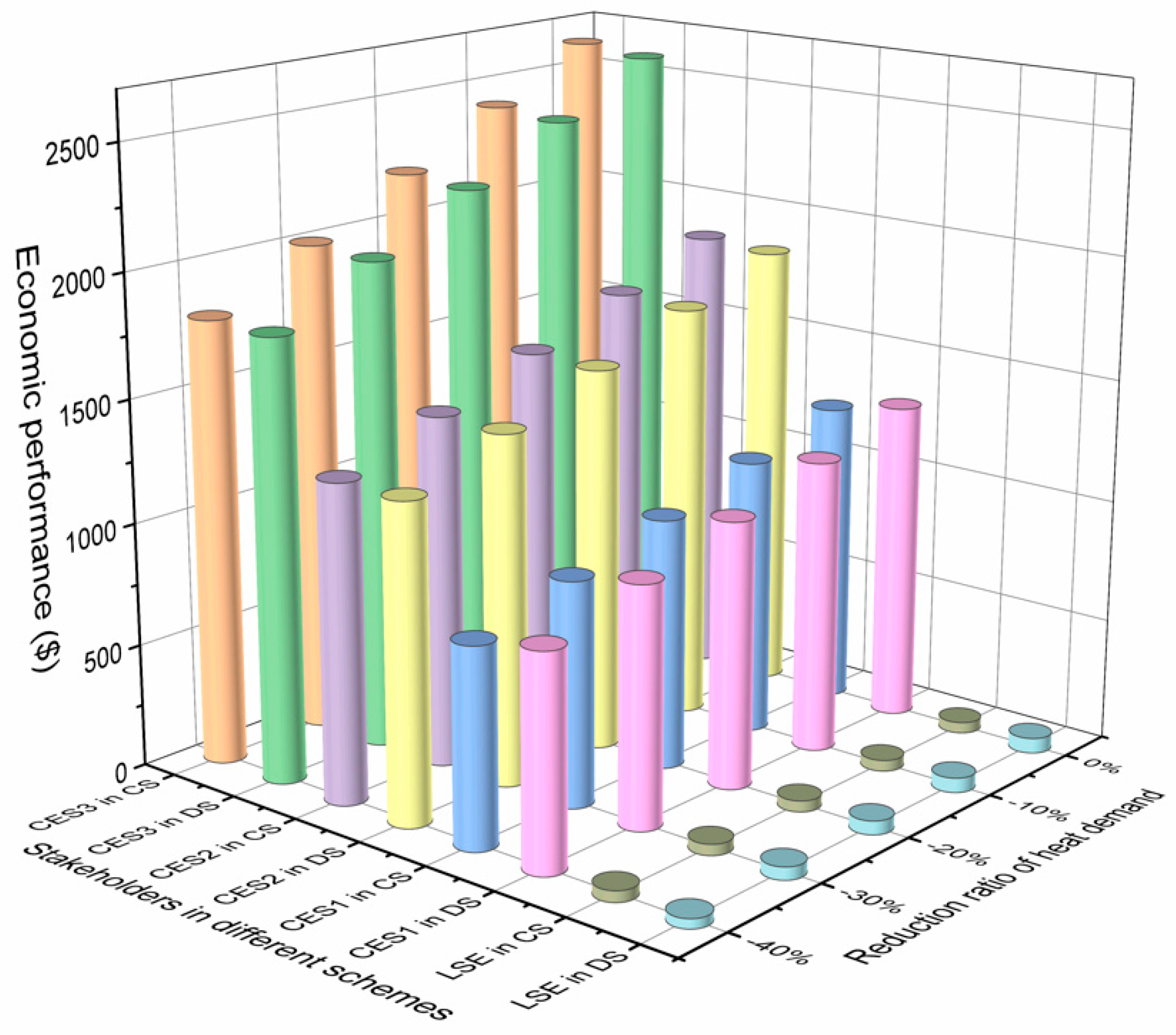
Figure 8 displays the profit allocation affected by dynamic energy load profiles in two coordination schemes. Because the electricity and heat load are both considered, the electricity load was fixed and the heat demand was changed like the above case. Due to the limitation of equipment capacity, the heat demand cannot increase. Therefore, the changing ratio was set from −40% to 0% as shown in Figure 8. When the heat demand decreases, it can be seen that the costs of all CESs decrease. All the costs are lower than those in the act alone scenario. It is interesting to note that the profit of LSE in the centralized scheme changes little, and that in the decentralized scheme the profit increases by 56.55% when the heat demand increases by 40%. This is mainly because the CHP systems generated more electricity and heat to meet the increase of heat demand. Then, the surplus electricity was traded among the CESs in the decentralized scheme according to the prices defined by the LSE. This situation can bring the LSE more profit compared with the low heat demand scenario.
Natural gas is the main fuel of energy systems consumed by the CHP systems and boilers. The cost of natural gas accounts for a large proportion of the total cost. Therefore, Figure 9 shows the costs and profit changed along with the variation of the natural gas price. Generally, it can be found that the costs of CESs illustrate an increasing trend and the profits of LSE illustrate a decreasing trend in both two coordination schemes, when the gas price increases. The profit decline of LSE was mainly due to a reduction in the energy interaction of CESs. The profit of LSE in the decentralized scheme reduced faster than that in the centralized scheme. It can be deduced that the LSE in the decentralized scheme was more sensitive to the gas prices. The performance of the LSE in the centralized scheme is robust accompanied by the variation of gas price.
6. Conclusions
In this paper, the energy interaction strategies among a load service entity and community energy systems are optimized, which is focused on a day-ahead trading scenario. Two coordination schemes are formulated. The first one is a centralized coordination scheme that the load service entity and community energy systems are fully cooperative to maximize social welfare. The other scheme is a decentralized coordination one formed as a Stackelberg game that the actors sequentially activate the resources based on other actors’ decisions. The mathematical models and solution methods are determined for each scheme. The Shapley value method, fair index, and DP value are applied for the profit allocation and stability test in a centralized coordination scheme. For the decentralized coordination scheme, a bilevel model is formulated based on the design process of each stakeholder. The internal electricity price is the medium for the coordination of the load service entity and community energy systems. Thus, the comprehensive assessment and sensitivity analysis are conducted to discuss the coordination in the centralized and decentralized coordination schemes.
Three cases are defined to study the effect of different coordination schemes on the dispatch strategies and economic performance of each stakeholder. The results indicate that the centralized and decentralized coordination schemes lead to a meaningful increase in social welfare. A win-win situation is formed in that both the load service entity and community energy systems benefit from the proposed two coordination schemes simultaneously. For the decentralized coordination scheme, the load service entity decides internal trading prices under a regulated environment. Adopting these interaction strategies under a decentralized framework, greater benefit obtained for one actor incurs no losses for other actors. From an economic perspective, the centralized coordination is slightly more advantageous in terms of cost minimization than the decentralized one. However, the reasonable allocation scheme may be difficult to form to satisfy the Core conditions, fair and stable constraints. Too many selfish individuals may create difficulties for implementing the centralized coordination scheme and forming a grand coalition, especially to establish a feasible, stable, and fair allocation scheme. Based on the consideration of economic performance and problem scale, a decentralized coordination scheme with a hierarchical structure is a good choice to implement in a real-life setting, which can avoid the unreasonable allocation scheme under a regulated environment. In this paper, the KKT condition and strong dual theory are used to address the optimization problem in the decentralized coordination scheme. In future work, the distributed approach can be considered to solve the bilevel problem.
Funding
This work was supported by the National Natural Science Foundation of China (71904179), Natural Science Foundation of Hubei province (2019CFB209), Fundamental Research Funds for the Central Universities, China University of Geosciences (Wuhan) (CUG170691).
Conflicts of Interest
The authors declare no conflict of interest.
Nomenclature
Abbreviations:
CHP
combined heat and power system
CES
community energy system
DP
propensity to disrupt
FI
fairness index
KKT
Karush-Kuhn-Tucker
LSE
load service entity
O&M
operation and maintenance
PV
photovoltaics
RTP
real-time pricing
WT
wind turbine
Index:
I
set of equipment in community energy systems
J
set of purchasing and selling electricity
Q
set of community energy systems
set of time periods
Parameters:
a given depth of discharge in storage
Initial stored energy in the storage in CES q in period t
,
locational marginal prices of electricity
natural gas purchasing price of the energy market during period t
,
electricity and heat demand in CES q during period t
maximum load curtailment limit
total cost of each CES that energy market prices are sent to the CES directly
,
upper and lower generation or storage capacity of equipment in CES q during period t
,
upper PV generation and electrical storage capacity in LSE during period t
,
maximum charging and discharging rate during period t
factor for adjusting the costs of the LSE and CESs
upper bound of hourly price changes in CES q
,
upper and lower bound of the hourly interaction prices in CES q
,,,,
O&M cost of CHP, PV, heat storage, electrical storage, and boiler in CES q during period t
load curtailment cost during period t
,
electricity and thermal efficiency of CHP in CES q during period t
,
charging and discharging efficiency of electrical storage in LSE.
,
upper and lower bounds of inputs and outputs of energy storage in CES q
loss percentage of storage in CES q
Variables:
internal electricity trading price during period t
the amount of electrical load curtailment
,
cost of LSE and CES q
,
electricity generated by CHP and PV in CES q during period t
,
heat generated by CHP and boiler in CES q during period t
,
heat stored in the storage, and heat input to/output from the thermal storage in CES q during period t
,
LSE purchasing and selling electricity from or to the utility grid during period t
,,
electricity generated by PV, and electricity charging and discharging quantity in LSE during period t
,
CES purchasing and selling electricity from or to the LSE during period t
Appendix A. KKT Condition
To transform the bilevel problem into a single level problem, the KKT condition is used as the CES’s problem and is linear and convex. By applying the KKT method, the decision variables in the LSE’s problem are considered as the parameters in the CES’s problem. In the following Equations is substituted in Equations (15) and (17) by in Equations (18) and (19). It is assumed that the energy stored in storage is zero at the initial period ().
Stationarity:
Complementary slackness conditions:
The dual variables are equal to or greater than zero, . In the above constraints, Equations (A26)–(A42) are nonlinear and can be replaced by Equation (A43). is the binary variable, and M is a sufficiently large positive coefficient.
Appendix B. Strong Dual Theory
In Equation (1), is nonlinear. Since the CES’s problem is convex, as acts as a parameter, the nonlinear expression can be substituted by a strong duality equation. The dual problem of the CES’s problem is constructed to linearize the nonlinear expression:
References
Manfren, M.; Caputo, P.; Costa, G. Paradigm shift in urban energy systems through distributed generation: Methods and models. Appl. Energy2011, 88, 1032–1048. [Google Scholar] [CrossRef]
Mendes, G.; Ioakimidis, C.; Ferrão, P. On the planning and analysis of Integrated Community Energy Systems: A review and survey of available tools. Renew. Sustain. Energy Rev.2011, 15, 4836–4854. [Google Scholar] [CrossRef]
Koirala, B.P.; Koliou, E.; Friege, J.; Hakvoort, R.A.; Herder, P.M. Energetic communities for community energy: A review of key issues and trends shaping integrated community energy systems. Renew. Sustain. Energy Rev.2016, 56, 722–744. [Google Scholar] [CrossRef]
Zhou, Y.; Wei, Z.; Sun, G.; Cheung, K.W.; Zang, H.; Chen, S. A robust optimization approach for integrated community energy system in energy and ancillary service markets. Energy2018, 148, 1–15. [Google Scholar] [CrossRef]
Li, B.; Roche, R.; Paire, D.; Miraoui, A. A price decision approach for multiple multi-energy-supply microgrids considering demand response. Energy2019, 167, 117–135. [Google Scholar] [CrossRef]
Hansen, T.M.; Roche, R.; Suryanarayanan, S.; Maciejewski, A.A.; Siegel, H.J. Heuristic optimization for an aggregator-based resource allocation in the smart grid. IEEE Trans. Smart Grid2015, 6, 1785–1794. [Google Scholar] [CrossRef]
Nguyen, D.T.; Nguyen, H.T.; Le, L.B. Dynamic pricing design for demand response integration in power distribution networks. IEEE Trans. Power Syst.2016, 31, 3457–3472. [Google Scholar] [CrossRef]
Nisan, N.; Roughgarden, T.; Tardos, E.; Vazirani, V.V. Algorithmic Game Theory; Cambridge University Press: Cambridge, UK, 2007. [Google Scholar]
Wu, Q.; Ren, H.; Gao, W.; Ren, J.; Lao, C. Profit allocation analysis among the distributed energy network participants based on Game-theory. Energy2017, 118, 783–794. [Google Scholar] [CrossRef]
Prete, C.L.; Hobbs, B.F. A cooperative game theoretic analysis of incentives for microgrids in regulated electricity markets. Appl. Energy2016, 169, 524–541. [Google Scholar] [CrossRef]
Han, L.; Morstyn, T.; McCulloch, M. Incentivizing Prosumer Coalitions With Energy Management Using Cooperative Game Theory. IEEE Trans. Power Syst.2019, 34, 303–313. [Google Scholar] [CrossRef]
Du, Y.; Wang, Z.; Liu, G.; Chen, X.; Yuan, H.; Wei, Y.; Li, F. A cooperative game approach for coordinating multi-microgrid operation within distribution systems. Appl. Energy2018, 222, 383–395. [Google Scholar] [CrossRef]
Dempe, S.; Dutta, J. Is bilevel programming a special case of a mathematical program with complementarity constraints? Math. Program.2012, 131, 37–48. [Google Scholar] [CrossRef]
Wang, Z.; Chen, B.; Wang, J.; Begovicn, M.M.; Chen, C. Coordinated Energy Management of Networked Microgrids in Distribution Systems. IEEE Trans. Smart Grid2015, 6, 45–53. [Google Scholar] [CrossRef]
Jalali, M.; Zare, K.; Seyedi, H. Strategic decision-making of distribution network operator with multi-microgrids considering demand response program. Energy2017, 141, 1059–1071. [Google Scholar] [CrossRef]
Bahramara, S.; Moghaddam, M.P.; Haghifam, M.R. A bi-level optimization model for operation of distribution networks with micro-grids. Int. J. Electr. Power Energy Syst.2016, 82, 169–178. [Google Scholar] [CrossRef]
Le Cadre, H.; Mezghani, I.; Papavasiliou, A. A game-theoretic analysis of transmission-distribution system operator coordination. Eur. J. Oper. Res.2019, 274, 317–339. [Google Scholar] [CrossRef]
Bard J, F. Practical Bilevel Optimization: Algorithms and Applications; Springer Science & Business Media Press: Berlin, Germany, 2013. [Google Scholar]
von Appen, J.; Braun, M. Strategic decision making of distribution network operators and investors in residential photovoltaic battery storage systems. Appl. Energy2018, 230, 540–550. [Google Scholar] [CrossRef]
Sadeghi Mobarakeh, A.; Rajabi-Ghahnavieh, A.; Haghighat, H. A bi-level approach for optimal contract pricing of independent dispatchable DG units in distribution networks. Int. Trans. Electr. Energy Syst.2016, 26, 1685–1704. [Google Scholar] [CrossRef]
Yazdani-Damavandi, M.; Neyestani, N.; Chicco, G.; Shafie-Khah, M.; Catalao, J.P. Aggregation of distributed energy resources under the concept of multienergy players in local energy systems. IEEE Trans. Sustain. Energy2017, 8, 1679–1693. [Google Scholar] [CrossRef]
Zhen, L.; Zhang, X.; Lieu, J. Design of the incentive mechanism in electricity auction market based on the signaling game theory. Energy2010, 35, 1813–1819. [Google Scholar]
Jin, M.; Feng, W.; Marnay, C.; Spanos, C. Microgrid to enable optimal distributed energy retail and end-user demand response. Appl. Energy2018, 210, 1321–1335. [Google Scholar] [CrossRef]
Barbose, G.; Goldman, C.; Neenan, B. A Survey of Utility Experience with Real Time Pricing; Lawrence Berkeley National Laboratory: Berkeley, CA, USA, 2004. [Google Scholar]
Kang, L.; Yang, J.; An, Q.; Deng, S.; Zhao, J.; Wang, H.; Li, Z. Effects of load following operational strategy on CCHP system with an auxiliary ground source heat pump considering carbon tax and electricity feed in tariff. Appl. Energy2017, 194, 454–466. [Google Scholar] [CrossRef]
Li, L.; Mu, H.; Li, N.; Li, M. Economic and environmental optimization for distributed energy resource systems coupled with district energy networks. Energy2016, 109, 947–960. [Google Scholar] [CrossRef]
Shapley, L.S.; Shubik, M. Game Theory in Economics: Chapter 6, Characteristic Function, Core, and Stable Set. 1973. Available online: https://www.rand.org/pubs/reports/R0904z6.html (accessed on 19 June 2020).
Dinar, A.; Howitt, R.E. Mechanisms for allocation of environmental control cost: Empirical tests of acceptability and stability. J. Environ. Manag.1997, 49, 183–203. [Google Scholar] [CrossRef]
Shapley, L.S.; Shubik, M. A method for evaluating the distribution of power in a committee system. Am. Political Sci. Rev.1954, 48, 787–792. [Google Scholar] [CrossRef]
Littlechild, S.C.; Vaidya, K. The propensity to disrupt and the disruption nucleolus of a characteristic function game. Int. J. Game Theory1976, 5, 151–161. [Google Scholar] [CrossRef]
Gately, D. Sharing the gains from regional cooperation: A game theoretic application to planning investment in electric power. Int. Econ. Rev.1974, 15, 195–208. [Google Scholar] [CrossRef]
Sharma, S.; Abhyankar, A.R. Loss allocation of radial distribution system using Shapley value: A sequential approach. Int. J. Electr. Power Energy Syst.2017, 88, 33–41. [Google Scholar] [CrossRef]
Sinha, S.; Sinha, S.B. KKT transformation approach for multi-objective multi-level linear programming problems. Eur. J. Oper. Res.2002, 143, 19–31. [Google Scholar] [CrossRef]
Dempe, S.; Kalashnikov, V.; Prez-Valds, G.A.; Kalashnykova, N. Bilevel Programming Problems: Theory, Algorithms and Applications to Energy Networks; Springer Publishing Company: Berlin, Germany, 2015. [Google Scholar]
Figure 1.
The underlying structure of the load service entity (LSE) and community energy systems (CESs).
Figure 1.
The underlying structure of the load service entity (LSE) and community energy systems (CESs).
Figure 2.
Load profiles in each CES.
Figure 2.
Load profiles in each CES.
Figure 3.
Electricity trading prices for each CES.
Figure 3.
Electricity trading prices for each CES.
Figure 4.
The economic performance of LSE and CES in each case. (Case 1: Act alone scenario; Case 2: Centralized coordination scheme; Case 3: Decentralized coordination scheme. The numbers on the column are the cost of each actor.).
Figure 4.
The economic performance of LSE and CES in each case. (Case 1: Act alone scenario; Case 2: Centralized coordination scheme; Case 3: Decentralized coordination scheme. The numbers on the column are the cost of each actor.).
Figure 5.
Optimal reduced cost allocation strategy in two schemes.
Figure 5.
Optimal reduced cost allocation strategy in two schemes.
Figure 6.
Energy dispatch strategies of CES2 under the decentralized coordination scheme: (a) electricity dispatch strategies; (b) heat dispatch strategies.
Figure 6.
Energy dispatch strategies of CES2 under the decentralized coordination scheme: (a) electricity dispatch strategies; (b) heat dispatch strategies.
Figure 7.
Effect of storage capacity variation on the economic benefit of stakeholders (CS: centralized coordination scheme; DS: decentralized coordination scheme).
Figure 7.
Effect of storage capacity variation on the economic benefit of stakeholders (CS: centralized coordination scheme; DS: decentralized coordination scheme).
Figure 8.
Effect of energy demand on the economic benefit of stakeholders (CS: centralized coordination scheme; DS: decentralized coordination scheme).
Figure 8.
Effect of energy demand on the economic benefit of stakeholders (CS: centralized coordination scheme; DS: decentralized coordination scheme).
Figure 9.
Influence of the natural gas price on the economic performance of the LSE and CESs: (a) centralized coordination scheme; (b) decentralized coordination scheme.
Figure 9.
Influence of the natural gas price on the economic performance of the LSE and CESs: (a) centralized coordination scheme; (b) decentralized coordination scheme.
Table 1.
Main operation parameters of LSE and CESs.
Table 1.
Main operation parameters of LSE and CESs.
Entity
(kW)
(kW)
(kW)
(kWh)
(kWh)
LSE
-
-
400
-
600
-
CES1
-
-
560
1850
-
-
CES2
800
0.3573
1260
5500
-
-
CES3
1460
0.3634
1960
5600
-
900
Table 2.
Costs of various coalitions.
Table 2.
Costs of various coalitions.
Coalitions
Cost ($)
Coalitions
Cost ($)
{LSE}
0.00
{CES1}
1336.06
{CES2}
1887.69
{CES3}
2643.95
{LSE, CES1}
1222.05
{LSE, CES2}
1843.52
{LSE, CES3}
2608.84
{CES1, CES2}
3122.99
{CES1, CES3}
3880.88
{CES2, CES3}
4523.02
{LSE, CES1, CES2}
3059.46
{LSE, CES1, CES3}
3802.76
{LSE, CES2, CES3}
4485.73
{CES1, CES2, CES3}
5737.36
{LSE, CES1, CES2, CES3}
5683.01
Table 3.
The cost allocation scheme based on cooperation.
Table 3.
The cost allocation scheme based on cooperation.
Centralized Coordination Scenario
LSE
CES1
CES2
CES3
Total
Cost Allocation ($)
−44.61
1243.21
1865.35
2619.06
5683.01
Fairness Index
0.61
DP value
0.22
−0.04
0.01
0.00
-
Table 4.
The cost allocation scheme based on non-cooperation.
Table 4.
The cost allocation scheme based on non-cooperation.
Li, L.
Optimal Coordination Strategies for Load Service Entity and Community Energy Systems Based on Centralized and Decentralized Approaches. Energies2020, 13, 3202.
https://doi.org/10.3390/en13123202
AMA Style
Li L.
Optimal Coordination Strategies for Load Service Entity and Community Energy Systems Based on Centralized and Decentralized Approaches. Energies. 2020; 13(12):3202.
https://doi.org/10.3390/en13123202
Chicago/Turabian Style
Li, Longxi.
2020. "Optimal Coordination Strategies for Load Service Entity and Community Energy Systems Based on Centralized and Decentralized Approaches" Energies 13, no. 12: 3202.
https://doi.org/10.3390/en13123202
APA Style
Li, L.
(2020). Optimal Coordination Strategies for Load Service Entity and Community Energy Systems Based on Centralized and Decentralized Approaches. Energies, 13(12), 3202.
https://doi.org/10.3390/en13123202
Note that from the first issue of 2016, this journal uses article numbers instead of page numbers. See further details here.
Article Metrics
No
No
Article Access Statistics
For more information on the journal statistics, click here.
Multiple requests from the same IP address are counted as one view.
Li, L.
Optimal Coordination Strategies for Load Service Entity and Community Energy Systems Based on Centralized and Decentralized Approaches. Energies2020, 13, 3202.
https://doi.org/10.3390/en13123202
AMA Style
Li L.
Optimal Coordination Strategies for Load Service Entity and Community Energy Systems Based on Centralized and Decentralized Approaches. Energies. 2020; 13(12):3202.
https://doi.org/10.3390/en13123202
Chicago/Turabian Style
Li, Longxi.
2020. "Optimal Coordination Strategies for Load Service Entity and Community Energy Systems Based on Centralized and Decentralized Approaches" Energies 13, no. 12: 3202.
https://doi.org/10.3390/en13123202
APA Style
Li, L.
(2020). Optimal Coordination Strategies for Load Service Entity and Community Energy Systems Based on Centralized and Decentralized Approaches. Energies, 13(12), 3202.
https://doi.org/10.3390/en13123202
Note that from the first issue of 2016, this journal uses article numbers instead of page numbers. See further details here.


