Selection of a Suitable Rheological Model for Drilling Fluid Using Applied Numerical Methods

Abstract

The accuracy of fitting the rheological model to the properties of actual drilling fluid minimises the errors of the calculated technological parameters applied while drilling oil wells. This article presents the methodology of selecting the optimum drilling fluid rheological model. Apart from classical rheological models, i.e., the Newtonian, Bingham Plastic, Casson, Ostwald de Waele and Herschel–Bulkley models, it has been proposed to consider the Vom Berg and Hahn-Eyring models, which have not been applied to describe drilling fluids so far. In the process of determining rheological parameters for the Bingham Plastic, Casson, Ostwald de Waele and Newtonian models, it is proposed to use a linear regression method. In the case of the Herschel–Bulkley, Vom Berg and Hahn-Eyring models, it is suggested to use a non-linear regression method. Based on theoretical considerations and mathematical relations developed in the Department of Drilling and Geoengineering, Drilling, Oil and Gas Faculty, at AGH University of Science and Technology, an original computer program called Rheosolution was developed, which enables automation of the process of determining the optimum drilling fluid rheological model. Some examples show the practical application of the method of selecting the optimum drilling fluid rheological model. Taking into account data from actual measurements of drilling fluid properties, it has been proven that the Vom Berg and Hahn-Eyring rheological models are best fitted to the description of drilling fluid rheological parameters.

1. Introduction

For over 150 years, different drilling fluids such as drilling muds, drill-in fluids, spacers and washers, cement slurries and fracturing fluids have been used in the drilling practice. Each of them has to fulfil strictly specified functions so that the borehole making process is safe both for the natural environment and people working on a drilling rig. For instance, drilling mud is aimed at cleaning the borehole bottom off drill cuttings, removing cuttings up to the area surface, ensuring the stability of borehole walls both during drilling and circulation breaks, protecting against eruption (by exerting hydrostatic pressure), maintaining cuttings in a state of suspension during breaks in circulation, cleaning teeth of a drilling tool, lubricating drill bearings, cooling down a drill, and at supplying energy to the borehole bottom in order to support the drilling process. In addition, during directional drilling, horizontal drilling and multilateral drilling, drilling mud provides drive to mud motors (PDM motors, turbine drilling motors, RSS systems) and enables control of the trajectory course (Measurement-While-Drilling systems).

Together with the development of new drilling technologies such as high pressure and high temperature (HPHT technology), underbalance drilling (UBD drilling), managed pressure drilling (MPD technology), it becomes more and more important to determine precisely drilling mud and drilling fluid parameters and properties. Technological properties of the applied fluids depend, inter alia, on their rheological parameters. In order to describe cause and effect relations occurring between rheological parameters of a fluid and the technology of its use, rheological models are developed. The knowledge of a fluid rheological model is crucial since the accuracy of fitting a rheological model to the actual property of fluid minimises errors of values being calculated, including the nature of the fluid flow, fluid flow resistance in the circulatory system, diameters of drilling or extending tool nozzles, mechanical and hydraulic parameters of the drilling technology, particle sedimentation and the effectiveness of cuttings removal, injection radius and the technology of its application (stream of flow volume, pressure and time of injection performance), power consumption during mixing, mixing efficiency and issues relating to thermal conductivity during flow and mixing.

A number of rheological models have been developed in the drilling practice, however, none of them is universal enough to describe precisely the behaviour of drilling fluids in a wide range of shear rates. Rheological models form a mathematical description of the behaviour of Newtonian fluids. Those models may be divided into two groups:

−

relations between the shear rate and shear stress,

−

relations between the shear rate or shear stress and apparent viscosity.

Models in both groups are different with respect to the applied function and parameters approximating actual fluid behaviour. Models from the first group are applied for the analysis of drilling fluids.

2. Rheological Models of Drilling Fluids

The following rheological models are most frequently applied for drilling technologies [1,2]:

$$\mathrm{Newtonian}: \tau =\eta \left(-\frac{dv}{dr}\right)$$

(1)

$$\mathrm{Bingham}: \tau ={\tau }_y+{\eta }_{pl}\left(-\frac{dv}{dr}\right)$$

(2)

$$\mathrm{Ostwald} \mathrm{de} \mathrm{Waele}: (\mathrm{Power} \mathrm{Law}): \tau =k{\left(-\frac{dv}{dr}\right)}^n$$

(3)

$$\mathrm{Casson}: {\tau }^{\frac{1}{2}}={\tau }_y^{\frac{1}{2}}+{\eta }_{cas}^{\frac{1}{2}}{\left(-\frac{dv}{dr}\right)}^{\frac{1}{2}}$$

(4)

$$\mathrm{Herschel}\text{-}\mathrm{Bulkley}: (\mathrm{Yield}\text{-}\mathrm{Power} \mathrm{Law}): \tau ={\tau }_y+k{\left(-\frac{dv}{dr}\right)}^n.$$

(5)

The Bingham Plastic model has been applied most frequently due to its relative simplicity and ease in calculating flow resistances [1]. Yet, at high shear rates and more complex drilling fluid formulas, particularly those using polymers, this model does not describe the nature of drilling fluids in a precise way.

When computers started to be used more commonly, it became possible to support computational processes commonly and numerically, which helped to popularise the power model and the Herschel—Bulkley model (YPL), which describes drilling fluids the best among those currently used in the drilling practice [3,4]. Presently, computers are commonly available, and their computational power enables the performance of quite complex and extended numerical calculations in a short time. Therefore, it seems reasonable to analyse other models, which could prove to be better than those applied so far, and the use of which could have been impractical so far, due to calculations complexity.

The Vom Berg model and the Hahn-Eyring model have been selected for the analysis [5,6]. The main selection criterion was another nature of the curve describing the dependency of shear stresses on the shear rate. Contrary to the Ostwald—de Waele (Powel Law) model and the Herschel—Bulkley (Yeld-Power Law) model, and also similar models, such as the Sisko model or the Robertson–Stiff model [6], the curve in the analysed models is described by an inverse hyperbolic function instead of a power function. The second criterion was very good results of applying those models in other industries, which would justify considering them in the context of describing drilling fluids by means of them. Both the Vom Berg model and the Hahn-Eyring model have successfully been applied to the description of cement slurries used in the construction industry, which is confirmed in the literature [6]. The last condition was potentially high flexibility and possibility to fit into measurement data. In this case (similarly to the YPL model), it is ensured by three parameters, which can be adapted to the fluid under analysis.

New Vom Berg and Hahn-Eyring models, proposed to be applied in the drilling sector, are described as follows [5,6,7]:

$$\mathrm{Vom} \mathrm{Berg}: \tau ={\tau }_y+D{\sinh }^{-1}\left(\frac{-\frac{dv}{dr}}{C}\right)$$

(6)

$$\mathrm{Hahn}\text{-}\mathrm{Eyring}: \tau =E\left(-\frac{dv}{dr}\right)+D{\sinh }^{-1}\left(\frac{-\frac{dv}{dr}}{C}\right).$$

(7)

The authors make an attempt to demonstrate the usefulness of the Vom Berg and Hahn-Eyring models (not used in calculations for drilling fluids yet) in minimising errors in the calculation of rheological parameters and, in consequence, more accurate determination of flow resistance of drilling fluids.

3. Methodology

Laboratory tests of real drilling fluids were performed by means of rotational viscometers. The result of those tests was a set of measurement points, in which values of shear stresses ($\tau$) occurring in the fluid under the influence of different shear rates ($\dot{\gamma }=\left(-\frac{dv}{dr}\right)$) were determined.

In order to determine the optimum rheological model, it has been suggested to conduct a regression analysis, since it specifies the most probable function linking average values of both variables. The procedure of determining a regression function is called the least-squares method. This principle boils down to the statement that among all functions illustrating dispersion of measurement results the best one is the one for which the sum of squares of measurement points deviations from that function is the lowest [8].

In the case of the Bingham Plastic, Casson, Ostwald de Waele and Newtonian models, the authors propose to apply a linear regression method. In case of the Herschel–Bulkley, Vom Berg and Hahn-Eyring models, they suggest applying a non-linear regression method.

3.1. Linear Regression

In the case of linear regression, the optimum function is expected to take the form of a linear Equation [8]:

$$\widehat{y}=ax+b.$$

(8)

The least squares estimation is presented in the following form:

$$U={\displaystyle \sum _{i=1}^m{\left(y_i-\widehat{y}\right)}^2\to \min }.$$

(9)

Taking into account Equation (8), a sum of squared residuals is obtained:

$$U={\displaystyle \sum _{i=1}^m\left(y_i^2-2a{x}_i{y}_i-2b{y}_i+a^2{x}_i^2+2ab{x}_i+b^2\right)\to \min }.$$

(10)

Equation (10) is a function of coefficients a and b. The condition of function U minimisation can be thus expressed in the form of the following equations:

$$\{\begin{array}{l}\frac{\partial U}{\partial a}=-2{\displaystyle \sum _{i=1}^m{x}_i{y}_i+2a{\displaystyle \sum _{i=1}^m{x}_i^2+2b{\displaystyle \sum _{i=1}^m{x}_i}=0}}\\ \frac{\partial U}{\partial b}=-2{\displaystyle \sum _{i=1}^m{y}_i+2a{\displaystyle \sum _{i=1}^m{x}_i+2bm=0}}\end{array}.$$

(11)

By solving a system of Equation (11), one can acquire formulas for linear regression coefficients, known from the literature:

$$a=\frac{{{\displaystyle \sum }}_{i=1}^m{x}_i{y}_i-{{\displaystyle \sum }}_{i=1}^m{x}_i{{\displaystyle \sum }}_{i=1}^m{y}_i}{{{\displaystyle \sum }}_{i=1}^m{x}_i{}^2-{\left({{\displaystyle \sum }}_{i=1}^m{x}_i\right)}^2}$$

(12)

$$b=\frac{{{\displaystyle \sum }}_{i=1}^m{y}_i-a{{\displaystyle \sum }}_{i=1}^m{x}_i}{m}$$

(13)

For the Bingham Plastic model, Equations (12) and (13) can be used directly, by applying substitutions: η = a, τ_y = b, $\dot{\gamma }$ = x and τ= y. Rheological parameters are determined from the following relation:

$$\eta =\frac{m{\displaystyle \sum _{i=1}^m{x}_i{y}_i-{\displaystyle \sum _{i=1}^m{x}_i{\displaystyle \sum _{i=1}^m{y}_i}}}}{m{\displaystyle \sum _{i=1}^m{x}_i^2-{\left({\displaystyle \sum _{i=1}^m{x}_i}\right)}^2}}$$

(14)

$${\tau }_y=\frac{{\displaystyle \sum _{i=1}^m{y}_i-\eta {\displaystyle \sum _{i=1}^m{x}_i}}}{m}.$$

(15)

For the Ostwald—de Waele (Power Law) model and the Casson model, their linearisation is necessary. Linearisation of the Ostwald—de Waele (Power Law) model is acquired by logarithmic Equation (3) on both sides as follows:

$$\ln \tau =\ln k+n\ln \dot{\gamma }$$

(16)

and using substitutions n = a, lnk = b, ln$\dot{\gamma }$ = x, lnτ = y.

Rheological parameters are determined from the following relation:

$$n=\frac{m{\displaystyle \sum _{i=1}^m{x}_i{y}_i-{\displaystyle \sum _{i=1}^m{x}_i{\displaystyle \sum _{i=1}^m{y}_i}}}}{m{\displaystyle \sum _{i=1}^m{x}_i^2-{\left({\displaystyle \sum _{i=1}^m{x}_i}\right)}^2}}$$

(17)

$$k=e^{\left(\frac{{\displaystyle \sum _{i=1}^m{y}_i-\eta {\displaystyle \sum _{i=1}^m{x}_i}}}{m}\right)}.$$

(18)

Linearisations of the Casson model are performed by applying substitutions: $\sqrt{{\eta }_{cas}}=a$, $\sqrt{{\tau }_y}=b$, $\sqrt{\dot{\gamma }}=x$ and $\sqrt{\tau }=y$. Rheological parameters are determined from the following relation:

$${\eta }_{cas}={\left(\frac{m{\displaystyle \sum _{i=1}^m{x}_i{y}_i-{\displaystyle \sum _{i=1}^m{x}_i{\displaystyle \sum _{i=1}^m{y}_i}}}}{m{\displaystyle \sum _{i=1}^m{x}_i^2-{\left({\displaystyle \sum _{i=1}^m{x}_i}\right)}^2}}\right)}^2$$

(19)

$${\tau }_y={\left(\frac{{\displaystyle \sum _{i=1}^m{y}_i-\sqrt{{\eta }_{cas}}{\displaystyle \sum _{i=1}^m{x}_i}}}{m}\right)}^2.$$

(20)

For the Newtonian model, when applying the least squares method, a regression function in the following form is assumed:

$$\widehat{y}=ax.$$

(21)

The least-squares condition given with Equation (9), taking into account Equation (21) is described with the formula:

$$U={\displaystyle \sum _{i=1}^m\left(y_i^2-2a{x}_i{y}_i+a^2{x}_i^2\right)\to \min }.$$

(22)

By differentiating Equation (22) against coefficient a, the following formula is obtained:

$$\frac{\partial U}{\partial a}=-2{\displaystyle \sum _{i=1}^m{x}_i{y}_i+2a{\displaystyle \sum _{i=1}^m{x}_i^2}}$$

(23)

from which, after comparing to zero, one can designate the value of coefficient a

$$a=\frac{{\displaystyle \sum _{i=1}^m{x}_i{y}_i}}{{\displaystyle \sum _{i=1}^m{x}_i^2}}.$$

(24)

A rheological parameter of the Newtonian model (dynamic viscosity η) is thus determined from the following relationship:

$$\eta =\frac{{\displaystyle \sum _{i=1}^m\left({\dot{\gamma }}_i{\tau }_i\right)}}{{\displaystyle \sum _{i=1}^m{\dot{\gamma }}_i^2}}.$$

(25)

3.2. Non-Linear Regression

The Herschel–Bulkley model cannot be linearised since while determining parameter equations an implicit equation with one variable occurs. The condition of function U minimisation can thus be expressed in the form of equations:

$$\{\begin{array}{l}\frac{\partial U}{\partial {\tau }_y}=-2{\displaystyle \sum _{i=1}^m{\tau }_i+2k{\displaystyle \sum _{i=1}^m{\dot{\gamma }}_i^n+2m{\tau }_y=0}}\\ \frac{\partial U}{\partial k}=-2{\displaystyle \sum _{i=1}^m{\tau }_i{\dot{\gamma }}_i^n+2{\tau }_y{\displaystyle \sum _{i=1}^m{\dot{\gamma }}_i^n+2k{\displaystyle \sum _{i=1}^m{\dot{\gamma }}_i^{2n}}}=0}\\ \frac{\partial U}{\partial n}=-2k{\displaystyle \sum _{i=1}^m({\tau }_i{\dot{\gamma }}_i^n\ln {\dot{\gamma }}_i)+2{\tau }_{y}k{\displaystyle \sum _{i=1}^m\left({\dot{\gamma }}_i^n\ln {\dot{\gamma }}_i\right)+2k^2{\displaystyle \sum _{i=1}^m\left({\dot{\gamma }}_i^{2n}\ln {\dot{\gamma }}_i\right)}}=0}\end{array}.$$

(26)

A system of Equation (26) after ordering variables boils down to the following form: [4]

$$\begin{array}{c}m {\displaystyle {\displaystyle \sum }_{i=1}^m}({\tau }_i{\dot{\gamma }}_i^n\ln {\dot{\gamma }}_i)-{\displaystyle {\displaystyle \sum }_{i=1}^m}{\tau }_i{\displaystyle {\displaystyle \sum }_{i=1}^m}({\dot{\gamma }}_i^n\ln {\dot{\gamma }}_i)+\\ \frac{m{\displaystyle \sum _{i=1}^m{\tau }_i{\dot{\gamma }}_i^n-{\displaystyle \sum _{i=1}^m{\tau }_i{\displaystyle \sum _{i=1}^m{\dot{\gamma }}_i^n}}}}{m{\displaystyle \sum _{i=1}^m{\dot{\gamma }}_i^{2n}-{\displaystyle \sum _{i=1}^m{\dot{\gamma }}_i^n{\displaystyle \sum _{i=1}^m{\dot{\gamma }}_i^n}}}}\left[{\displaystyle \sum _{i=1}^m{\dot{\gamma }}_i^n}{\displaystyle \sum _{i=1}^m\left({\dot{\gamma }}_i^n\ln {\dot{\gamma }}_i\right)}-m{\displaystyle \sum _{i=1}^m\left({\dot{\gamma }}_i^{2n}\ln {\dot{\gamma }}_i\right)}\right]=0.\end{array}$$

(27)

Equation (27) is an implicit equation with one variable n. In order to solve it, it is suggested to apply one of the numerical methods, e.g., the bisection method [9].

In this method, a function is constructed in the following form: [4]

$$\begin{array}{c}g(n)=m{\displaystyle \sum _{i=1}^m({\tau }_i{\dot{\gamma }}_i^n\ln {\dot{\gamma }}_i)-{\displaystyle \sum _{i=1}^m{\tau }_i}{\displaystyle \sum _{i=1}^m\left({\dot{\gamma }}_i^n\ln {\dot{\gamma }}_i\right)}}+\\ \frac{m{\displaystyle \sum _{i=1}^m{\tau }_i{\dot{\gamma }}_i^n-{\displaystyle \sum _{i=1}^m{\tau }_i{\displaystyle \sum _{i=1}^m{\dot{\gamma }}_i^n}}}}{m{\displaystyle \sum _{i=1}^m{\dot{\gamma }}_i^{2n}-{\displaystyle \sum _{i=1}^m{\dot{\gamma }}_i^n{\displaystyle \sum _{i=1}^m{\dot{\gamma }}_i^n}}}}\left[{\displaystyle \sum _{i=1}^m{\dot{\gamma }}_i^n}{\displaystyle \sum _{i=1}^m\left({\dot{\gamma }}_i^n\ln {\dot{\gamma }}_i\right)}-m{\displaystyle \sum _{i=1}^m\left({\dot{\gamma }}_i^{2n}\ln {\dot{\gamma }}_i\right)}\right]\end{array}$$

(28)

and next zero is designated.

To this end, at the beginning, the range [A, B] is established, within which the existence of the root being searched for is predicted. Considering the physical sense of the parameter n being searched for, one can assume n ∈ [0, 100]. The principle of designating the zero of the g(n) function in the range [A, B] by means of the bisection method is as follows (Figure 1):

The starting range [A, B] is divided into two in order to determine the value of the coordinate of the interval centre: $n_{sr}=\frac{A+B}{2}$. Next, the value of the g(n_sr) function is determined and compared to the g(A) value. If the function changes the sign, it means that the root of the g(n) function is in the range [A, n_śr]; otherwise, the root is in the range [n_śr, B]. Calculations are made until the range width is smaller or equal to accuracy ε assumed at the beginning. The root of the function is then determined based on the formula: $n_{sr}=\frac{A+B}{2}$, whereas the error of its estimation is calculated from the dependency: $\mathrm{blad}=\frac{B-A}{2}$.

The algorithm of Equation (28), with the use of the bisection method, has been provided in Figure 2.

Given the designated value of the parameter n, the other rheological parameters in the Herschel-Bulkley model can be specified from Equations (29) and (30):

$$k=\frac{m{\displaystyle \sum _{i=1}^m{\tau }_i{\dot{\gamma }}_i^n-{\displaystyle \sum _{i=1}^m{\tau }_i{\displaystyle \sum _{i=1}^m{\dot{\gamma }}_i^n}}}}{m{\displaystyle \sum _{i=1}^m{\dot{\gamma }}_i^{2n}-{\displaystyle \sum _{i=1}^m{\dot{\gamma }}_i^n{\displaystyle \sum _{i=1}^m{\dot{\gamma }}_i^n}}}}$$

(29)

$${\tau }_y=\frac{{\displaystyle \sum _{i=1}^m{\tau }_i-k{\displaystyle \sum _{i=1}^m{\dot{\gamma }}_i^n}}}{m}.$$

(30)

Similarly, to the Herschel-Bulkley (YPL) model, also in the case of the Vom Berg and Hahn-Eyring models, linearisation of their rheological equations is not possible:

The condition of the function U minimisation for the Vom Berg model, using substitutions

$$a={\tau }_y, b=D, c=C, y_i={\tau }_i, x_i=-{\left(\frac{dv}{dr}\right)}_i$$

can be expressed in the form of a system of equations:

$$\{\begin{array}{c}\frac{\partial U}{\partial a}=2{{\displaystyle \sum }}_{i=1}^m\left(b{\sinh }^{-1}\left(\frac{x_i}{c}\right)\right)-2{{\displaystyle \sum }}_{i=1}^m{y}_i+2am=0\\ \frac{\partial U}{\partial b}={{\displaystyle \sum }}_{i=1}^m\left(-2{\sinh }^{-1}\left(\frac{x_i}{c}\right)\left(-a-b{\sinh }^{-1}\left(\frac{x_i}{c}\right)+y_i\right)\right)=0\\ \frac{\partial U}{\partial c}={{\displaystyle \sum }}_{i=1}^m\frac{2b{x}_i\left(-a-b{\sinh }^{-1}\left(\frac{x_i}{c}\right)+y_i\right)}{c^2\sqrt{1+\frac{x_i^2}{c^2}}}=0\end{array}.$$

(31)

The condition of the function U minimisation for the Hahn-Eyring model, by applying substitutions

$$a=E, b=D, c=C, y_i={\tau }_i, x_i=-{\left(\frac{dv}{dr}\right)}_i$$

can be expressed in the form of a system of equations:

$$\{\begin{array}{c}\frac{\partial U}{\partial a}={{\displaystyle \sum }}_{i=1}^m(-2x_i\left(-a{x}_i-b{\sinh }^{-1}\left(\frac{x_i}{c}\right)+y_i)\right)=0\\ \frac{\partial U}{\partial b}={{\displaystyle \sum }}_{i=1}^m\left(-2{\sinh }^{-1}\left(\frac{x_i}{c}\right)\left(-a{x}_i-b{\sinh }^{-1}\left(\frac{x_i}{c}\right)+y_i\right)\right)=0\\ \frac{\partial U}{\partial c}={{\displaystyle \sum }}_{i=1}^m\frac{2b{x}_i\left(-a{x}_i-b{\sinh }^{-1}\left(\frac{x_i}{c}\right)+y_i\right)}{c^2\sqrt{1+\frac{x_i^2}{c^2}}}=0\end{array}.$$

(32)

There are a number of available non-linear regression methods [10,11]. With regard to the Vom Berg and Hahn-Eyring models, it is proposed to apply gradient descent [12]. This algorithm enables us to find local minima of a function and to determine the global minimum from among them. It consists of selecting a starting point to be found in the domain of the analysed function. This function is a function which specifies fitting of the analysed model equation (the sum of squared residuals) and designates a vector in it with the direction of a given function gradient and the sense opposite to it. The length of a step (vector) is equal to one multiplied by the vector length coefficient. This coefficient can be freely adapted to optimise the algorithm:

$$U\left(a,b,c\right)={\displaystyle \sum }_{i=1}^n{\left(f\left(a,b,c\right)-y_i\right)}^2\to \min$$

(33)

$$\widehat{v}=\frac{-\overrightarrow{\nabla }U\left(a,b,c\right)}{\left|-\overrightarrow{\nabla }U\left(a,b,c\right)\right|}·{\alpha }_k.$$

(34)

After the computational sequence has been performed, the model parameters are modified with the vector value and the algorithm selects a given point as a new starting point. The process is repeated until a local minimum is achieved, with the assumed precision. Then, the starting point changes and another local minimum is searched for. After repeating calculations, the assumed number of times, the smallest of the local minima being found is selected and considered the global minimum.

The flow chart of calculations is presented in Figure 3 and Figure 4.

To simplify the equation, particular rheological model parameters are ascribed to variables $a, b, c$, whereas constant $y_i$ and $x_i$ are data from subsequent measurement points. With every step, only the variables are modified. Assignment of model equations to the diagram:

$$\mathrm{the} \mathrm{Vom} \mathrm{Berg} \mathrm{model}: \tau ={\tau }_y+D{\sinh }^{-1}\left(\frac{-\frac{dv}{dr}}{C}\right)$$

$$a={\tau }_y, b=D, c=C, y_i={\tau }_i, x_i=-{\left(\frac{dv}{dr}\right)}_i$$

$$U\left(a,b,c\right)={\displaystyle \sum }_{i=1}^m{\left(f\left(a,b,c\right)-y_i\right)}^2={\displaystyle \sum }_{i=1}^m{\left(a+b{\sinh }^{-1}\left(\frac{x_i}{c}\right)-y_i\right)}^2\to \min$$

(35)

$$\mathrm{the} \mathrm{Hahn}\text{-}\mathrm{Eyring} \mathrm{model}: \tau =E\left(-\frac{dv}{dr}\right)+D{\sinh }^{-1}\left(\frac{-\frac{dv}{dr}}{C}\right)$$

$$a=E, b=D, c=C, y_i={\tau }_i, x_i=-{\left(\frac{dv}{dr}\right)}_i$$

$$U\left(a,b,c\right)={\displaystyle \sum }_{i=1}^m{\left(f\left(a,b,c\right)-y_i\right)}^2={\displaystyle \sum }_{i=1}^m{\left(a{x}_i+b{\sinh }^{-1}\left(\frac{x_i}{c}\right)-y_i\right)}^2\to \min$$

(36)

Partial derivatives are calculated according to Equation (31) or Equation (32). The gradient descent can be also applied when designating rheological parameters under the Herschel-Bulkley model.

3.3. Numerical Support of the Process of Selecting a Drilling Fluid Rheological Model

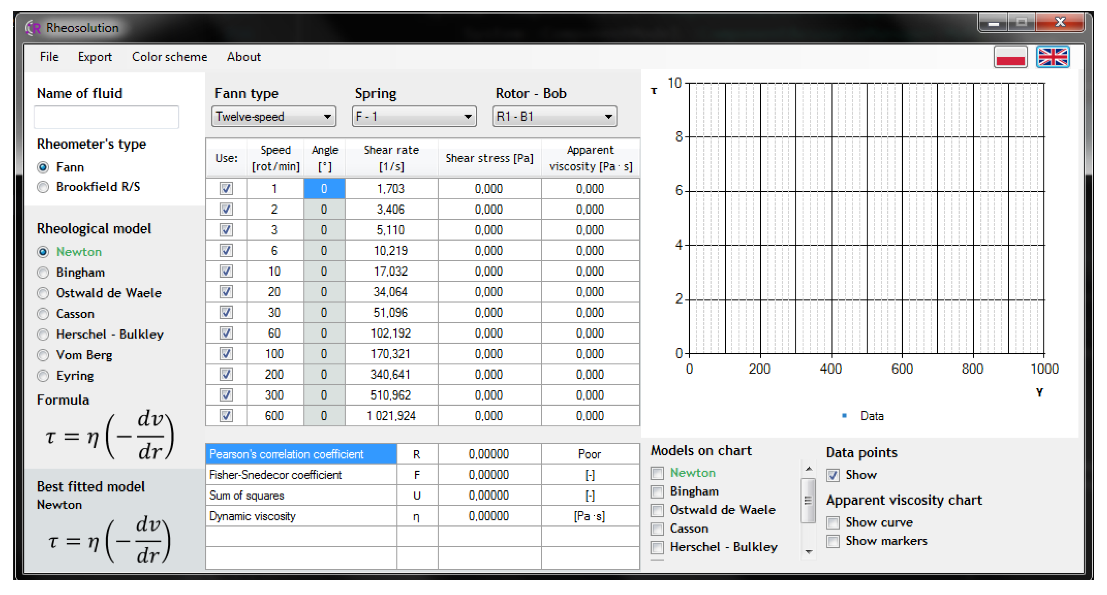
Development of the methodology of fitting rheological parameters in research data has enabled us to create a numerical tool making it possible to select the optimum drilling fluid rheological model. A new version of the Rheosolution program, version 4.0, has been developed, in which apart from the Newtonian, Bingham Plastic, Ostwald–de Waele, Casson and Herschel–Bulkley models, handling of the Vom Berg model and the Hahn-Eyring model was introduced. A number of other changes were made, including, inter alia, modernisation and reconstruction, together with rewriting the program from the Pascal language into C++/CLI and also adding the English version.

Rheosolution in the new version 4.0 adapts the parameters of seven rheological models to the measurement data being introduced. The program calculates rheological parameters for each of the analysed models and indicates the model with the highest degree of fitting. Data and diagrams are exported to files, images and spreadsheets.

The way of fitting rheological parameters depends on a model. In case of the Newtonian and Bingham Plastic models, linear regression is applied, which enables designation of linear equation parameters. Ostwald–de Waele and Casson equations are linearised, and next, linear regression is applied. The last three models are designated by means of gradient descent.

The user interface has been provided in Figure 5. The method of program operation is shown in Figure 6.

4. Results and Discussion

In order to exemplify the relations presented in this article, laboratory tests of different drilling fluids were made [1]. The measurements were made in the Drilling Fluids Laboratory in the Department of Drilling and Geoengineering, Faculty of Drilling, Oil and Gas on a Fann viscometer. The tested fluids were the following:

• Cement slurry o w/c = 0.5, without any additives,
• Cement slurry o w/c = 0.5 with addition of 0.3% PSP 042 superplasticizer,
• 3% bentonite drilling mud without any additives.
• 3% bentonite drilling mud with an addition of 2% XCD polymer.

Table 1. Data from laboratory tests made on a Fann viscometer (R1-B1, F1).

Cement w/c 0.5		With Addition of PSP 042		3% Drilling Mud		With Addition of 2% XCD
Rotations	Angle	Rotations	Angle	Rotations	Angle	Rotations	Angle
rot/min	°	rot/min	°	rot/min	°	rot/min	°
1	12	1	2	1	3	1	23
2	15	2	2	2	4	2	24
3	18	3	3	3	5	3	26
6	25	6	4	6	6	6	28
10	32	10	6	10	6	10	31
20	47	20	10	20	6	20	35
30	54	30	14	30	6	30	38
60	67	60	28	60	8	60	45
100	80	100	48	100	10	100	51
200	108	200	91	200	14	200	65
300	132	300	141	300	18	300	76
600	183	600	237	600	28	600	98

shows the results of rheological measurements of four drilling fluid formulas performed on a Fann viscometer, with the arrangement of Rotor-Bob cylinders (R1-B1) and an applied spring (F1) [1].

Table 2. Relations between shear stresses and shear rates obtained from laboratory tests on a Fann viscometer (R1-B1, F1).

Cement w/c 0.5		With Addition of PSP 042		3% Drilling Mud		With Addition of 2% XCD
Shear Rate	Tension	Shear Rate	Tension	Shear Rate	Tension	Shear Rate	Tension
1/s	Pa	1/s	Pa	1/s	Pa	1/s	Pa
1.7034	6.132	1.7034	1.022	1.7034	1.533	1.7034	11.753
3.4068	7.665	3.4068	1.022	3.4068	2.044	3.4068	12.264
5.1102	9.198	5.1102	1.533	5.1102	2.555	5.1102	13.286
10.2204	12.775	10.2204	2.044	10.2204	3.066	10.2204	14.308
17.034	16.352	17.034	3.066	17.034	3.066	17.034	15.841
34.068	24.017	34.068	5.11	34.068	3.066	34.068	17.885
51.102	27.594	51.102	7.154	51.102	3.066	51.102	19.418
102.204	34.237	102.204	14.308	102.204	4.088	102.204	22.995
170.34	40.88	170.34	24.528	170.34	5.11	170.34	26.061
340.68	55.188	340.68	46.501	340.68	7.154	340.68	33.215
511.02	67.452	511.02	72.051	511.02	9.198	511.02	38.836
1022.04	93.513	1022.04	121.107	1022.04	14.308	1022.04	50.078

shows relations between shear stresses and the shear rate obtained from laboratory tests on a Fann viscometer, with the arrangement of Rotor-Bob cylinders (R1-B1) and an applied spring (F1) [1].

Table 3. Fluid rheological parameters obtained from Rheosolution 4.0 for cement slurry samples (with and without adding superplasticizer).

		Cement w/c 0.5		With Addition of PSP 042
Newtonian	η = 0.1105	-	-	η = 0.1246	-	-
Bingham	ηpl = 0.0842	τy = 16.9723	-	ηpl = 0.1215	τy = 1.9507	-
Ostwald—de Waele	k = 4.7932	n = 0.4265	-	k = 0.3931	n = 0.8012	-
Casson	ηcas = 0.0532	τy = 8.7314	-	ηcas = 0.1159	τy = 0.1668	-
Herschel- Bulkley	k = 2.2527	n = 0.5420	τy = 1.2854	k = 0.2925	n = 0.8718	τy = 0.1440
Vom Berg	τy = 9.8527	D = 26.5833	C = 105.2867	τy = 0.0165	D = 96.9329	C = 643.4336
Hahn-Eyring	E = 0.0922	D = 1.6225	C = 0.7939	E = 0.1146	D = 0.9401	C = 1.0184

and

Table 4. Fluid rheological parameters obtained from Rheosolution 4.0 for drilling mud samples (with and without adding polymer).

		3% Drilling Mud		With Addition of 2% XCD
Newtonian	η = 0.0159	-	-	η = 0.0622	-	-
Bingham	ηpl = 0.0119	τy = 2.5903	-	ηpl = 0.0377	τy = 15.8508	-
Ostwald—de Waele	k = 1.3046	n = 0.2959	-	k = 8.9200	n = 0.2241	-
Casson	ηcas = 0.0057	τy = 1.7405	-	ηcas = 0.0145	τy = 11.8160	-
Herschel-Bulkley	k = 0.1682	n = 0.6217	τy = 1.3479	k = 4.6678	n = 0.3285	τy = 2.8143
Vom Berg	τy = 0.4649	D = 1.8184	C = 9.2868	τy = 12.6203	D = 11.5721	C = 98.7531
Hahn-Eyring	E = 0.0086	D = 0.6916	C = 1.0548	E = 0.0244	D = 2.4781	C = 0.0507

present the calculated values of rheological parameters pertaining to fluids under analysis, approximated with particular rheological models.

Table 5. Results of the rheological model selection obtained from Rheosolution 4.0 for drilling fluid samples (with and without adding polymer).

	3% Drilling Mud			With Addition of 2% XCD
Model/Coefficient	R	F	U	R	F	U
Newtonian	0.77745	15.27968	59.73121	0	0	2256.306
Bingham	0.99074	532.5236	2.78326	0.96043	118.8995	123.9423
Ostwald—de Waele	0.92387	58.27622	22.11583	0.97087	164.1754	91.72426
Casson	0.99554	1113.56	1.34393	0.99417	849.8189	18.58076
Herschel-Bulkley	0.98992	488.5667	3.02866	0.98816	414.6451	37.62234
Vom Berg	0.88438	35.90033	32.89705	0.99375	792.1389	19.91689
Hahn-Eyring	0.98781	402.6485	3.65926	0.99679	1547.903	10.25482

and

Table 6. Results of the rheological model selection obtained from Rheosolution 4.0 for cement slurry samples (with and without adding superplasticizer).

	Cement w/c 0.5			With addition of PSP 042
Model/Coefficient	R	F	U	R	F	U
Newtonian	0.77729	15.26429	3214.332	0.99534	1066.001	143.4055
Bingham	0.95144	95.52491	769.5607	0.99639	1378.773	111.1078
Ostwald—de Waele	0.99855	3449.434	23.47425	0.98011	243.846	607.8673
Casson	0.97705	210.3658	368.5144	0.99716	1750.87	87.62985
Herschel- Bulkley	0.98691	374.3877	211.2646	0.99874	3975.655	38.71535
Vom Berg	0.99009	496.8507	160.2201	0.99956	11232.52	13.7246
Hahn-Eyring	0.90418	44.80884	1481.655	0.99692	1616.03	94.89674

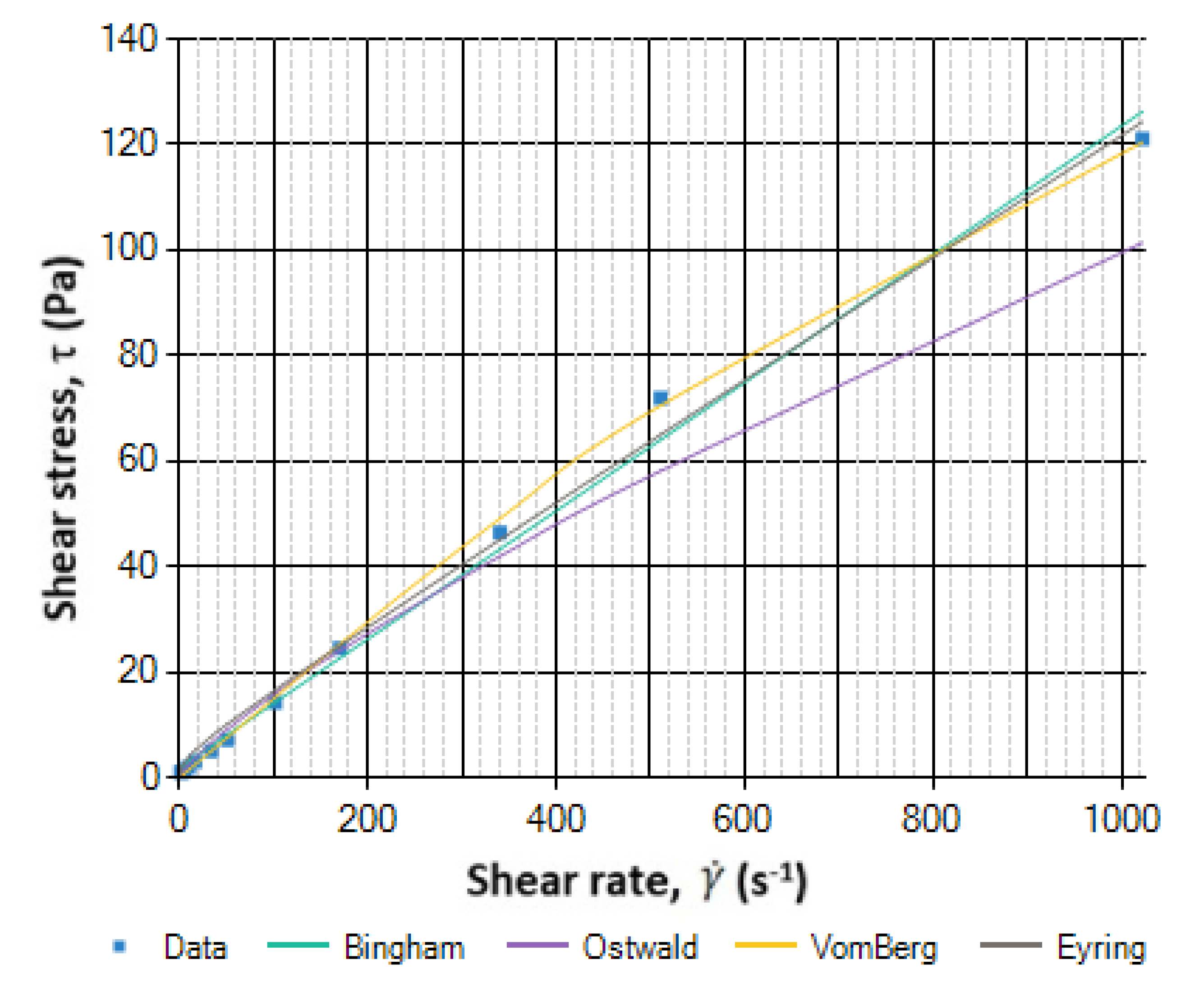
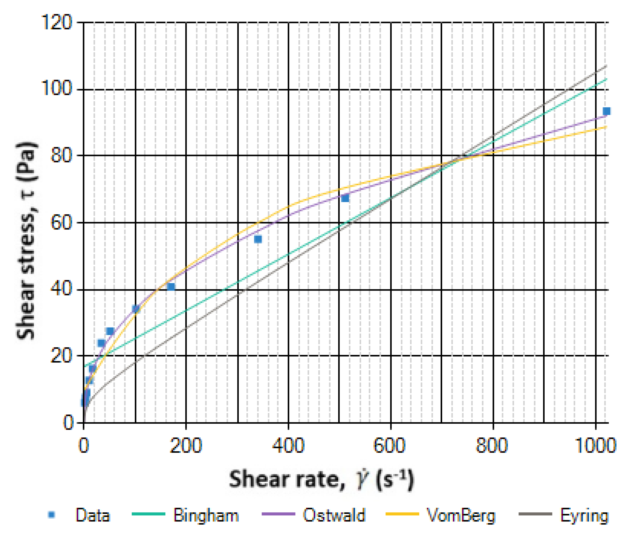
present rheological model selection results, pertaining to the analysed fluids, obtained from Rheosolution. Figure 7, Figure 8, Figure 9 and Figure 10 present drawings to show a comparison of the selected rheological models for the tested drilling mud and cement slurry. To maintain the clarity of the drawing, models recommended by the American Petroleum Institute (Bingham Plastic and Ostwald de Waele models) were selected for comparison.

The tests were successful. In the case of pure slurry, the Ostwald–de Waele model turned out to be the best-fitted model. For slurry with addition of PSP 042 superplasticizer, the Vom Berg model was the best fitted model. Pure bentonite drilling mud was best described by means of the Casson model, and polymer inhibited mud, by means of the Hahn-Eyring model. For drilling muds and cement slurries without additives, differences between the correlation coefficient are not that significant among some models and linear models have a good correlation in these cases.

Preliminary studies on sample drilling mud and cement slurries encourage more accurate analysis; the results indicate that the multi-parameter models of Vom Berg and Hahn-Eyring have a high correlation for drilling fluids with an addition of polymers or superplasticizers. This is due to the fact that such additions most often cause non-linear increases in the value of rheological parameters, therefore, models based on exponential functions better illustrate these changes. The use of computational methodology, Rheosolution 4.0 and viscometers such as Brookfield R/S (multi shear rate measurement points) can improve the adjustment of a rheological model to the behaviour of the actual drilling fluid during its flow.

Recently, progress has been made in the use of nanoparticles as an addition to drilling fluids in order to adjust their rheological parameters. Authors [13,14] emphasise in their works that the Power Law model or the Herschel Bulkley model can be used to predict drilling fluids behaviour during flow, whereas the application of the Bingham Plastic model can sometimes only capture the trend. This is a group of new drilling fluids which might require further studies to optimise the best mathematical model. The issue seems to be interesting and worth analysing since these drilling fluids, as indicated in some papers [15,16], describe exponential models well and such rheological models include also the Vom Berg and Hahn-Eyring models.

5. Conclusions

For many years, different drilling fluids such as drilling muds, drill-in fluids, spacers and washes, cement slurries and fracturing fluids have been applied in the drilling practice. Each kind of drilling fluid should be described with the best fitted rheological model. The accuracy of fitting a rheological model to the properties of actual fluid minimises errors in values being calculated, such as the nature of fluid flow, fluid flow resistances in the circulatory system, diameters of drilling or extending tool nozzles, mechanical and hydraulic parameters of the drilling technology, particle sedimentation and the effectiveness of cuttings removal, injection radius and the technology of its application (stream of flow volume, pressure and time of injection performance), power consumption during mixing, mixing efficiency and issues relating to thermal conductivity during flow and mixing.

The methodology developed and presented in this article enables us to select the optimum rheological model of any drilling fluid. In the process of designating rheological parameters for the Bingham Plastic, Casson, Ostwald de Waele and Newtonian models, it is proposed to apply a linear regression method. In the case of the Herschel–Bulkley, Vom Berg and Hahn-Eyring models, it is suggested to apply a non-linear regression method.

An interesting issue seems to be the use of the Vom Berg and the Hahn-Eyring rheological models to describe the flow of drilling fluids with an addition of nanoparticles [13,14,15,16] and this will be one of the later stages in the work of the authors of this article. We draw such conclusions on the basis of observations that multi-parameter models better describe the flow of liquids modified with chemical additives (superplasticizers, polymers).

The original Rheosolution computer program, developed in the Department of Drilling and Geoengineering, Drilling, Oil and Gas Faculty, at AGH University of Science and Technology, enables automation of the process of designating the optimum drilling fluid rheological model. Owing to the mathematical analysis conducted in this study and numerical calculations, taking into account data from actual measurements of drilling fluid properties, it has been proven that the Vom Berg and Hahn-Eyring rheological models fit best to describe drilling fluid rheological parameters. It is worthwhile to take subsequent steps in order to further test those models in terms of their usefulness in the drilling industry.

References

- API RP 13D. Rheology and Hydraulics of Oil-well Drilling Fluids; Norm of American Petroleum Institute: Washington, DC, USA, 2006. [Google Scholar]
- Bourgoyne, A.T.; Milheim, K.K.; Chenevert, M.E.; Young, F.S. Applied Drilling Engineering. In SPE Textbook; SPE: Houston, TX, USA, 1986; 4.8. [Google Scholar]
- Klotz, J.A.; Brigham, W.E. To Determine Herschel-Bulkley Coefficients. J. Pet. Technol. 1998, 50, 80–81. [Google Scholar] [CrossRef]
- Wiśniowski, R. Zastosowanie modelu Herschela-Bulkleya w hydraulice płuczek wiertniczych. Nowoczesne Techniki i Technologie Bezwykopowe. Zeszyt nr 2/2000 Kraków 2000, 20–28. [Google Scholar]
- Bair, S. Actual Eyring Models for Thixotropy and Shear-Thinning: Experimental Validation and Application to EHD. J. Tribol. 2004, 126, 728–732. [Google Scholar] [CrossRef]
- Pellegrino, C.; Faleshini, F. Sustainability Improvements in the Concrete Industry: Use of Recycled Materials for Structure Concrete Production; 2016 Technology & Engineering; Springer International Publishing: Cham, Switzerland, 2016; pp. 37–43. [Google Scholar]
- Vom Berg, W. Influence of specific surface and concentration of solids upon the fow behaviour of cement pastes. Mag. Concr. Res. 1979, 31, 211–216. [Google Scholar] [CrossRef]
- Rawlings, J.O.; Pentula, S.G.; Dickey, D.A. Applied Regression Analysis: A Research Tool, 2nd ed.; Springer: New York, NY, USA, 1998. [Google Scholar]
- Azure, I.; Aloliga, G.; Doabil, L. Comparative Study of Numerical Methods for Solving Non-linear Equations Using Manual Computation. Math. Lett. 2019, 5, 41–46. [Google Scholar] [CrossRef]
- Bazaraa, M.S.; Sherali, H.S.; Shetty, C.M. Nonlinear Programing—Theory and Algorithms, 3rd ed.; John Wiley & Sons, Inc.: Hoboken, NJ, USA, 2006. [Google Scholar]
- Luenberger, D.G.; Yinyu, Y. Linear and Nonlinear Programming, 4th ed.; Springer Science+Business Media, LLC: New York, NY, USA, 2008; pp. 14–19. [Google Scholar]
- Boyd, S.; Vandenberghe, L. Convex Optimization; United States of America by Cambridge University Press: New York, NY, USA, 2004. [Google Scholar]
- Boyou, N.V.; Ismail, I.; Sulaiman, W.R.W.; Sharifi Haddad, A.; Husein, N.; Hui, H.T.; Nadaraja, K. Experimental investigation of hole cleaning in directional drilling by using nano-enhanced water-based drilling fluids. J. Pet. Sci. Eng. 2019, 176, 220–231. [Google Scholar] [CrossRef]
- Sharma, M.M.; Zhang, R.; Chenevert, M.E. A new family of nanoparticle-based drilling fluids. In Proceedings of the SPE Annual Technical Conference and Exhibition, San Antonio, TX, USA, 8–10 October 2012; pp. 1–13. [Google Scholar]
- Smith, S.R.; Rafati, R.; Sharifi Haddad, A.; Cooper, A.; Hamidi, H. Application of aluminium oxide nanoparticles to enhance rheological and filtration properties of water-based muds at HPHT conditions Colloids Surfaces A Physicochem. Eng. Asp. 2018, 537, 361–371. [Google Scholar] [CrossRef]
- Rafati, R.; Smith, S.R.; Sharifi Haddad, A.S.; Novara, R.; Hamidi, H. Effect of nanoparticles on the modifications of drilling fluids properties: A review of recent advances Colloids Surfaces A Physicochem. Eng. Asp. 2018, 161, 61–76. [Google Scholar]
Figure 1.
Determination of the root of the g(n) function by means of the bisection method.
Figure 2.
Flow chart for the calculation of the root of the g(n) function within the interval [A, B] by means of the bisection method.
Figure 3.
Flow chart determining the function minimum.
Figure 4.
Schematic diagram of the non-linear programming method.
Figure 5.
Rheosolution 4.0 interface.
Figure 6.
Rheosolution 4.0 block diagram.
Figure 7.
Comparison of the selected rheological models, cement w/c 0.5.
Figure 8.
Comparison of the selected rheological models, cement w/c 0.5 with an addition of PSP 042.
Figure 9.
Comparison of the selected rheological models, 3% drilling mud.
Figure 10.
Comparison of the selected rheological models, 3% drilling mud with an addition of 2% XCD.