Abstract
State estimation of distribution systems typically relies on measurement sets with very low redundancy levels. In this paper, this fact is exploited by first solving a conventional load flow, using exclusively a critical set of measurements, and then compensating the solution to account for the few redundant measurements available. This leads to a suboptimal but sufficiently accurate estimate. It is shown how the sparse triangular factorization of the load flow Jacobian matrix can be fully exploited throughout the compensation-based procedure, preventing in this way the ill-conditioning associated with the gain matrix arising in the conventional least-squares formulation. Simulation results are provided for measurement configurations customarily found in distribution systems, showing the potential advantages of the proposed methodology.
1. Introduction
Advanced distribution management systems (ADMS) are expected to host very sophisticated operational tools, capable of tackling the numerous challenges posed by upcoming active distribution networks. It is well known that the State Estimator (SE) is the cornerstone on which any other ADMS application is based [1]. Using topological information, network parameters, and the available measurements and pseudo-measurements sets for each loading/generating scenarios, the SE determines the most likely state of the system [2].
Recent studies have carried out a careful revision of the state of the art on Distribution System State Estimation (DSSE) [3,4,5]. Those works analyze the most relevant challenges that utilities have to overcome in order to obtain all the benefits provided by SEs. The most troublesome lies in the need to increase the level of available measurements, most times confined to High Voltage (HV)/ Medium Voltage (MV) substations and a few more measurements scattered along the feeders (usually at MV/MV regulating/switching substations) [6,7] and secondary distribution transformers [8]. This lack of redundancy still continues today, due to the large extension of distribution networks and the huge cost that fully telemetering such large networks would imply. This limitation has been usually circumvented by resorting to so-called load allocation schemes, aimed at inferring critical pseudo-measurements at secondary substations (power flows injections) [9,10]. The load allocation problem has been substantially enriched by the advent of Advanced Measurement Infrastructure (AMI), including smart meters, as this equipment provides an indirect measurement of the complex powers demanded downstream secondary substations, possibly including an estimation of Low Voltage (LV) power losses. References [11,12,13], along with several others reviewed in [4], make use of these new information sources for the sake of improving the observability of distribution systems. Despite this fruitful line of research, mainly focused on improving the quality of pseudo measurements, and, despite the trend to increase the deployment of system monitoring devices, DSSE will continue to commonly face low redundancy measurement systems in the short term, and will remain so in the medium term [5,14].
Another relevant challenge is that associated with the capability of DSSEs to cope with several sources of ill-conditioning, usually linked to distribution systems, such as [2]: a large proportion of injection measurements, very short and long lines simultaneously ending at the same bus, and very large weighting factors used to enforce virtual measurements. This is in addition to the well-known natural ill-conditioning of the gain matrix arising in Weighted Least-Squares (WLS) estimators. The ill-conditioning of the gain matrix may cause both convergence problems and inaccurate estimates, as thoroughly discussed in [15,16,17]. Furthermore, many of the available measurements at these levels are currents rather than powers [18], leading to additional numerical issues typically deteriorating the performance of DSSEs (see chapter 9 of [2] for more details).
Mainly for those reasons, notable research efforts have been directed towards the design of alternative, WLS-based DSSE formulations, specifically tailored to distribution power networks with radial topology, some of them based on branch current state variables instead of the traditional bus voltages [19,20,21,22,23,24,25,26].
The current trend towards fully automated distribution systems, based on robust, yet low redundancy monitoring systems, encourages the search for ad hoc SE solutions, better suited to those boundary constraints. This paper is focused on developing a new procedure for DSSE characterized by its simplicity, while at the same time retaining the capability to cope with all factors encountered at these voltage levels: low redundancy of measurements, handling of current measurements and risk of ill-conditioning. The goal is to reach a good compromise between accuracy and numerical robustness. The basic idea after the proposed solution method, which is also the main contribution of this work, consists of using a simpler and robust power flow tool as a first step, and then compensating the preliminary load flow solution to account for the remaining redundant measurements, not yet used by the load flow solver. This leads to a suboptimal yet accurate enough solution, which can be easily implemented on any type of distribution network, balanced or unbalanced, radially operated or meshed, as long as the measurement redundancy remains relatively low.
The paper is organized as follows: the next section discusses the context in which DSSEs are typically applied, which motivates the proposed methodology. Section 3 and Section 4 present the mathematical framework on which the compensation method is based and the resulting algorithm, respectively. Next, Section 5 presents simulation results obtained with several benchmark systems, followed by the concluding remarks.
2. Motivation
This paper focuses on, but is not restricted to European MV networks, which are typically three-phase balanced systems. Figure 1 illustrates the topology, main components, and most commonly available measurements for these distribution systems.
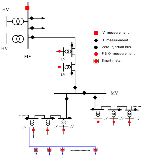
Figure 1.
One-line diagram of a typical European MV network.
Three types of substations can be found at this level [27]: the HV/MV primary substation, switching substations, which can include MV/MV regulating transformers in some cases, and MV/LV secondary substations. MV feeders leave HV/MV substations to reach consumers and distributed generators connected to secondary substations through typically shorter LV feeders. Most times, MV systems are planned with a ring or network topology, but they are radially operated for simplicity of protections, even though a meshed operational topology is also possible [28,29].
Regarding the monitored electrical quantities, all readings from smart meters downstream of LV feeders are collected by data concentrators located at secondary substations, constituting a good set of pseudomeasurements for the power delivered on the LV side of transformers. In addition, some utilities are investing in monitoring strategically selected secondary substations, where the power flows at the LV side of transformers are directly measured, rather than being the sum of downstream smart meters [30]. It is most important also to duly consider the exact zero-injection measurements at those nodes where neither consumers nor distributed generators are connected to, which are typically the MV sides of secondary transformers. All these injections (directly or indirectly measured), along with the voltage measurement at the MV bus of the primary substation, constitute a critical set of measurements that are the common input data to run the load flow tool.
State estimators are of interest when redundant measurements are added to the former critical set. These extra measurements are mainly concentrated at primary substations, specifically at the head of feeders where current magnitudes are traditionally recorded. A few additional current measurements, scattered downstream along the feeders (at certain MV/MV substations, voltage regulators locations, intermediate reclosers, etc.) [18] can also be available and used by the SE. Anyway, unlike in transmission systems, enjoying redundancy levels easily exceeding 4, current distribution systems barely exceed 1.15 (i.e., only 15% redundant measurements).
Note that all the previously commented pseudo-measurements, exact null injections, and real-time measurements have very different weighting factors associated, which causes ill-conditioning problems in conventional WLS-based SEs. Other relevant sources of problems, as discussed above, are the co-existence of long feeders and very short sections incident at the same bus (for example, some underground/overhead line segments can be a few meters long in urban networks), or the high proportion of power injections in the set of available measurements.
3. Proposed Method: Theoretical Background
As discussed above, for the low redundancy levels typically arising in distribution systems, it makes sense to divide the entire set of measurements into two disjoint subsets, namely: , representing a critical subset of n measurements allowing the n components of the state vector to be computed unambiguously; , representing the remaining subset of r measurements, redundant by nature, where typically (unlike in transmission systems). Both sets of measurements are related to the unknown state vector through nonlinear measurement functions, as follows:
where and are the vectors of measurement errors, assumed Gaussian and independent, characterized by the diagonal covariance matrices and , respectively.
Let us assume initially that the redundant measurements are missing. Then, we could resort to a load flow solver to obtain the state vector, , exactly satisfying the set of critical measurements, , i.e.,
By applying the Newton’s method, this involves the repeated solution of the following linear system, until is sufficiently small:
where k represents the iteration counter, is the Jacobian of , and
is the mismatch or residual vector, which becomes null at the solution.
When both types of measurements (critical and redundant) are simultaneously considered, the optimal estimate is obtained by repeatedly solving the well-known Normal Equations (NE) arising from the Gauss–Newton iterative method:
where
is the residual vector of the redundant measurements, and , represent the customary weighting matrices, accounting for the respective measurement uncertainties. Note that the dependence of the Jacobian matrices on the current state, , has been dropped for simplicity of notation.
Let the NE be rearranged as follows:
If we replace in Equation (7) by the fully converged load flow solution (), then , yielding:
where is the residual vector of the redundant measurements, computed at the load flow solution, , provided by the critical measurements. For convenience, we introduce at this point the following elements:
- An auxiliary vector:
- An auxiliary matrix:
Based on the above definitions, the system Equation (8) can be more compactly written as follows:
Note that matrix K can be very efficiently obtained by rows (i.e., columns of ) through repeated forward/backward solutions with the sparse triangular (or ) factors of (the load flow Jacobian available from the last iteration), namely by successively solving:
for every row i of .
Substituting from Equation (9) into the definition of y leads to the following reduced system:
and, rearranging:
The above system involves a dense coefficient matrix, but its size is small (), in accordance with the low redundancy levels available in distribution systems. Given a load flow solution, and the resulting , y can be obtained from Equation (12), which in turn allows computing from Equation (9). This constitutes the main contribution of the paper.
Solving Equation (9) can be interpreted as performing an additional load flow iteration, in which the mismatch vector is non null as a consequence of the redundant measurements. Obviously, owing to nonlinearities and measurement noise, the updated (compensated) state vector
will not correspond exactly to the optimal solution , obtained by successively iterating with Equation (5), but its accuracy may be sufficient for practical purposes, and in any case much better than that obtained when the redundant measurements are fully ignored. Note that, in the ideal or theoretical case in which all measurements were exact, both and y would be null, and there would be no need to compensate the load flow solution.
A major advantage of performing load flow compensated solutions is that they involve factorizing only the Jacobian matrix , which is several orders of magnitude better conditioned than the WLS gain matrix (). See [2] for a description of the main sources affecting the ill-conditioning of the NE.
4. Practical Implementation: Post-Compensating the Load Flow Solution
The following approximate procedure may provide sufficiently good solutions for practical purposes, particularly when the whole set of measurements can be rearranged so that contains the more accurate subset:
Figure 2 shows a flow diagram to help the reader visualize the major steps of the proposed method, including the iterative process of the load flow problem Equation (4). It is worth noting that, unlike in a regular load flow problem, where practical solution adjustments should be duly considered, such as enforcement of reactive power limits, in this case, such subtleties are not needed.
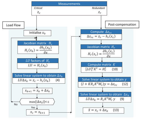
Figure 2.
Flow diagram of the proposed methodology.
In order to be able to run the load flow, which is the basic and most important hypothesis on which the proposed method is based, we need at least a pair of independent measurements for each bus. For the feeder head bus, we assume a voltage (V) measurement and take the angle as phase reference (). For the remaining buses, we assume that both P and Q measurements are available (possibly in the form of null-injection constraints), but in the presence of a distributed generator we could alternatively have P and V measurements, much like in transmission systems. If any V measurement is missing, we can simply use V = 1 as a pseudo-measurement, or the V measurement of a nearby bus, if available. If a P measurement is rather missing, we can replace it by a forecasted value, as the loads typically follow a repetitive daily pattern (this fact is very well known and widely exploited in power systems, for security analysis, etc.). Finally, if a Q measurement is missing, we can use the typical power factor of loads (e.g., ), depending on whether they are residential, industrial, etc., to generate a reasonable pseudo-measurement.
5. Results
Experiments comparing the proposed method with the conventional WLS SE are presented and discussed in this section. Both algorithms have been programmed in Matlab R2017a (MathWorks, Natick, MA, USA) and run on a 64-bit Intel Core i7 processor (2.8 GHz, 8 GB of RAM) (Intel, Santa Clara, CA, USA).
For the different scenarios, the corresponding sets of measurements have been generated from a load flow solution (considered as the exact network state for comparison purposes), to which Gaussian noise compatible with the standard deviation of each measurement is added.
The scenarios are built by considering the types of measurements usually deployed at the distribution levels: voltage magnitude at the head busbar, plus injections of active and reactive powers at the remaining load nodes. These critical sets have been completed with a variable number of current flow measurements randomly distributed throughout the network branches. For a given number of redundant current measurements, 100 different simulations are carried out, each differing in the branches where those measurements are located.
The standard deviations associated with the measurement errors are 0.0025 pu for the voltage magnitudes and power injections, and 0.01 pu for the current measurements. Virtual measurements (at zero-injection buses), unless otherwise indicated, are modeled as very exact measurements with a standard deviation of .
The convergence threshold is for all iterative processes (load flow and conventional SE).
Four networks ranging in size from 85 to over 3000 buses are tested in the sequel. The reader is referred to elsewhere regarding the detailed information fully characterizing those networks [31,32,33]. Table 1 summarizes the relevant parameters which can be helpful to understand the difficulties encountered when running the DSSE, namely: rated voltage, base power, total current flow at the head bus and branch impedances with maximum and minimum absolute magnitudes.

Table 1.
Parameters of the tested networks.
5.1. Convergence and Condition Number
The condition number evaluates the numerical ill-conditioning of a linear system of equations. In the poorly conditioned systems (i.e., those with a very large condition number), the numerical errors can impact the solution to the extent that the convergence rate is severely impaired. In extreme cases, the coefficient matrix cannot simply be factored, preventing a solution to be reached.
First, a large 3239-bus network [31], with 200 current flow measurements included (redundancy 1.03), is tested. This network is a structurally poorly-conditioned system, which means that its parameters are the source of ill-conditioning. This happens when very short branches (low impedances) coexist with long branches (large impedances). Table 2 shows the condition numbers arising for the different algorithms.
Table 2.
Condition number for the tested networks.
When running a conventional state estimator with this network, ill-conditioning problems appear in the factorization of equation system (5): the condition number reaches a very large value 1.4 × , which prevents from an estimated state to be computed in any of the scenarios tested.
However, when running the proposed compensated load flow solution, the condition number is drastically reduced, and the convergence is reached in all tested cases. A total of four iterations are needed by the load flow to converge, with a condition number of . In the additional iteration, at the compensation stage Equation (12), the condition number is × .
Another factor that significantly affects the condition number is the weights assigned to the zero-injection virtual measurements. Since those measurements are ‘exact’ (null injections), they are incorporated with a very low standard deviation, leading to a much larger weight than those assigned to the conventional measurements. This increases the numerical ill-conditioning of Equation (5).
Next, a real radial distribution network of 690 buses is tested. This network contains of zero-injection buses [33]. The critical set of load flow measurements has been supplemented with 30 current flow measurements (redundancy 1.02). Three different standard deviations for the virtual (exact) measurements are simulated, namely , and .
When running the conventional state estimator with the lowest weight (), all simulated scenarios converge, requiring an average of 3.9 iterations, with a condition number of . However, when the weights of virtual measurements are increased (), convergence and ill-conditioning problems appear when solving Equation (5). In this case, when the algorithm converges, the average number of iterations increases to 8.7, and the condition number rises up to . In of the simulations, the WLS problem cannot be solved. If the standard deviation of the virtual measurements is further reduced to , the ill-conditioning generalizes and none of the scenarios can be solved.
As opposed to the conventional WLS state estimator, the proposed compensated load flow converges for all the simulated scenarios, regardless of the weights associated with the virtual measurements. The load flow stage converges in four iterations, plus the final extra iteration of the compensation stage. Once again, the condition number of the equation systems gets significantly reduced. For the load flow stage, the condition number is 6 × ; for the small equation system Equation (12) of the final stage, the condition number is just 81.
In addition to the networks tested in this section, Table 2 gathers the condition numbers of two smaller systems (85 and 117 buses) that will be tested in the following sections. For the latter networks, 10 current flow measurements have been considered when computing the condition number. As can be seen, in all cases, the proposed methodology gives rise to condition numbers significantly lower than those obtained with a conventional state estimator.
5.2. Accuracy Analysis
This section compares the accuracy of the compensated load flow solution with that of the conventional state estimator.
For this purpose, two MV distribution feeders are analyzed, namely an 85-bus network [32], and a 117-bus system [31]. In the 85-bus network, the number of current flow (redundant) measurements included in the different scenarios is increased from 1 to 30, whereas, in the 117-bus system, the redundant measurements are increased in 10 steps, each comprising 10 current measurements, up to 100 measurements. For each redundancy level, 1000 different tests (with random current measurement location) are carried out.
Figure 3 shows the average absolute differences of the estimated voltage magnitudes and phase angles (in radians), with respect to the exact simulated values, for the 85-bus network scenarios. Figure 4 presents similar results for the 117-bus system. In order to show the improvement achieved by the correcting stage of the proposed algorithm, the average absolute errors arising after the first stage (just load flow computations based on critical sets) are shown with the red line.
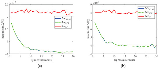
Figure 3.
85-bus system: (a) accuracy of voltage magnitudes; (b) accuracy of voltage phase angles (rad).
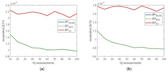
Figure 4.
117-bus system: (a) accuracy of voltage magnitudes; (b) accuracy of voltage phase angles (rad).
The results clearly show the increased accuracy attained when more and more redundant current measurements are added, which somehow saturates after a threshold is exceeded. They also confirm that the suboptimal estimate obtained with the compensated solution is almost indistinguishable from the one provided by the conventional state estimator.
5.3. Computational Cost
In this section, the computational effort of both the conventional state estimator and the compensated load flow is compared. Table 3 presents the execution time per iteration required by each algorithm, as well as the number of iterations (in brackets). As mentioned before, the conventional state estimator could not reach a solution for the 3239-bus network due to ill conditioning problems.
Table 3.
Execution time per iteration (s).
Further experiments have been performed for the 85-bus and the 117-bus systems. Regarding the convergence rate, Figure 5 shows the average number of iterations employed by a conventional state estimator, as the number of redundant current measurements increases. It can be observed that the higher the redundancy, the larger the number of iterations, reaching four iterations for the 85-bus network, and up to six iterations for the 117-bus system.
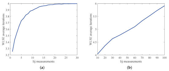
Figure 5.
Average iterations of the conventional state estimator: (a) 85-bus system; (b) 117-bus system.
On the other hand, the extended load flow involves only three iterations for the load flow stage, plus the additional iteration compensating the load flow solution, in all simulated cases. It is worth stressing that, in the proposed method, the current measurements are incorporated at this last stage and, therefore, the number of iterations of the preliminary load flow solution is not affected by the redundancy level.
Figure 6 shows the solution times required by both methodologies. As can be observed, there are no significant differences between both algorithms, regardless of the amount of current measurements considered. The compensated load flow method linearly increases the solution time with the number of redundant measurements. In any case, the total solution times are sufficiently small for this factor not to become the most relevant one in practice.
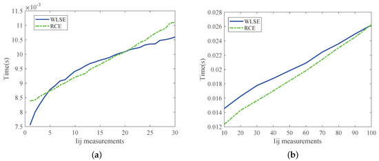
Figure 6.
Average computational cost: (a) 85-bus system; (b) 117-bus system.
5.4. Incorporation of Additional Measurements
In previous sections, the scenarios considered have been generated by adding a set of current flow measurements to the critical set of measurements used by the load flow. The proposed methodology is, however, not limited to the case in which the redundant set is composed of current measurements only. In this section, scenarios incorporating also extra voltage measurements are analyzed.
For the 85-bus network, in addition to the critical measurements associated with the load flow problem, 10 voltage magnitudes and 10 current flow measurements are incorporated, randomly distributed throughout the network. One hundred different scenarios, with different random locations, are performed.
The conventional estimator shows a condition number of × , while the condition number of the compensated load flow keeps at × at the first stage, and × at the second. Both methodologies employ a similar number of iterations: an average of 3.95 iterations for the conventional state estimator, and four iterations for the proposed method. The solution time is also similar: ms for the conventional state estimator versus 9 ms for the compensated load flow. The accuracy of both methodologies is also comparable, being the average absolute error × for the voltage magnitudes, and × radians for the phase angles.
6. Conclusions
This paper has examined the possibility of enhancing the results provided by a load flow solver, at minimum complexity and computational cost, with the information provided by a relatively small set of redundant measurements, a situation commonly arising in distribution systems. The goal is to attain estimates of similar accuracy as those provided by a conventional WLS estimator, while at the same time circumventing the severe ill-conditioning problems frequently found at those voltage levels. Simulation results have shown that the compensated load flow proposed in this work significantly reduces the condition number of the equation systems involved in the state estimation process. This way, the proposed methodology can successfully manage extremely ill-conditioned scenarios, where a conventional state estimator fails badly to obtain a solution. Moreover, the accuracy of the solution provided by the proposed algorithm has proved to be comparable to that of the conventional state estimator, while the computational cost is not an issue as long as the measurement redundancy remains low.
Author Contributions
Conceptualization and methodology, editing and supervision, A.G.-E.; software development and testing, C.G.-Q.; data curation and model validation, E.R.-R.; experimental design and analysis of results, A.d.l.V.-J.; all authors contributed to writing—original draft preparation. All authors have read and agreed to the published version of the manuscript.
Funding
This research was funded by the Spanish Ministerio de Ciencia e Innovacion (CDTI), under the CERVERA program for Outstanding Research Centers (CER-20191019) and by the 2020 PAIDI plan managed by the Consejeria de Economia y Conocimiento within the EU-FEDER Andalusia 2014-20 program (project S2V, US-1265887).
Conflicts of Interest
The authors declare no conflict of interest.
References
- Boardman, E. Advanced Applications in an Advanced Distribution Management System: Essentials for Implementation and Integration. IEEE Power Energy Mag. 2020, 18, 43–54. [Google Scholar] [CrossRef]
- Abur, A.; Gomez-Exposito, A. Power System State Estimation. Theory and Implementation; Marcel Dekker, Inc.: New York, NY, USA, 2004. [Google Scholar]
- Primadianto, A.; Lu, C. A Review on Distribution System State Estimation. IEEE Trans. Power Syst. 2017, 32, 3875–3883. [Google Scholar] [CrossRef]
- Dehghanpour, K.; Wang, Z.; Wang, J.; Yuan, Y.; Bu, F. A Survey on State Estimation Techniques and Challenges in Smart Distribution Systems. IEEE Trans. Smart Grid 2019, 10, 2312–2322. [Google Scholar] [CrossRef]
- New York State Energy Research and Development Authority (NYSERDA). Fundamental Research Challenges for Distribution State Estimation to Enable High-Performing Grids; NYSERDA Report Number 18-37; Smarter Grid Solutions: New York, NY, USA, 2018. Available online: https://www.nyserda.ny.gov/-/media/Files/Publications/Research/Electic-Power-Delivery/18-37-Fundamental-Research-Challenges.pdf (accessed on 14 June 2020).
- Xiang, Y. Operation of Future Medium Voltage Distribution Grids: Application of Statistical Methods for State Estimation and Fault Location. Ph.D. Thesis, Technische Universiteit Eindhoven, Eindhoven, The Netherlands, 2015. Available online: https://research.tue.nl/en/publications/operation-of-future-medium-voltage-distribution-grids-application (accessed on 14 June 2020).
- CIRED. Working Group on Smart Secondary Substations Technology Development and Distribution System Benefits; CIRED’s point of view Final Report; CIRED: Paris, France, 2017. [Google Scholar]
- Mauri, G.; Pilo, F.; Taylor, J.; Bruno, G.; Kampf, E.; Silvestro, F.; Pecas Lopez, C.; Bak-Jensen, B.; Pillai, J.R.; Sprongl, H. Control and Automation Systems for Electricity Distribution Networks (Edn) of the Future; CIGRE (International Council on Large Electric Systems): Paris, France, 2017. [Google Scholar]
- Carmona-Delgado, C.; Romero-Ramos, E.; Riquelme-Santos, J. Fast and Reliable Distribution Load and State Estimator. Electr. Power Syst. Res. 2013, 101, 110–124. [Google Scholar] [CrossRef]
- Arritt, R.; Dugan, R. Comparing Load Estimation Methods for Distribution System Analysis. In Proceedings of the International Conference on Electricity Distribution, Stockholm, Sweden, 10–13 June 2013. [Google Scholar]
- Lo, Y.; Huang, S.; Lu, C. Transformational Benefits of AMI Data in Transformer Load Modeling and Management. IEEE Trans. Power Deliv. 2014, 29, 742–750. [Google Scholar] [CrossRef]
- Alam, S.; Natarajan, B.; Pahwa, A. Distribution grid state estimation from compressed measurements. IEEE Trans. Smart Grid 2014, 5, 1631–1642. [Google Scholar] [CrossRef]
- Muscas, C.; Pau, M.; Pegoraro, P.; Sulis, S. Effects of measurements and pseudomeasurements correlation in distribution system state estimation. IEEE Trans. Instrum. Meas. 2014, 63, 2813–2823. [Google Scholar] [CrossRef]
- Dubey, A.; Bose, A.; Liu, M.; Ochoa, L.N. Paving the Way for Advanced Distribution Management Systems Applications: Making the Most of Models and Data. IEEE Power Energy Mag. 2020, 18, 63–75. [Google Scholar] [CrossRef]
- Lin, W.M.; Teng, J.H. State estimation for distribution systems with zero-injection constraints. IEEE Trans. Power Syst. 1996, 11, 518–524. [Google Scholar] [CrossRef]
- Muscas, C.; Pau, M.; Pegoraro, P.A.; Sulis, S. An efficient method to include equality constraints in branch current distribution system state estimation. Eurasip J. Adv. Signal Process. 2015, 2015, 1–11. [Google Scholar] [CrossRef]
- Nusrat, N. Development of Novel Electrical Power Distribution System State Estimation and Meter Placement Algorithms Suitable for Parallel Processing. Ph.D. Thesis, Brunel Institute of Power Systems (BIPS) Department of Electronic and Computer Engineering, London, UK, 2015. [Google Scholar]
- Roytelman, I. Real-time Distribution Power Flow—Lessons from practical implementations. In Proceedings of the 2006 IEEE PES Power Systems Conference and Exposition, Atlanta, GA, USA, 29 October–1 November 2006; pp. 505–509. [Google Scholar]
- Baran, M.E.; Kelley, A.W. A branch-current-based state estimation method for distribution systems. IEEE Trans. Power Syst. 1995, 10, 483–491. [Google Scholar] [CrossRef]
- Lin, W.-M.; Teng, J.-H.; Chen, S.-J. A highly efficient algorithm in treating current measurements for the branch-current-based distribution state estimation. IEEE Trans. Power Del. 2001, 16, 433–439. [Google Scholar] [CrossRef]
- Teng, J.-H. Using voltage measurements to improve the results of branch-current-based state estimators for distribution systems. IEE Proc. Gener. Transm. Distrib. 2002, 149, 667–672. [Google Scholar] [CrossRef]
- Deng, Y.; He, Y.; Zhang, B. A Branch-Estimation-Based State Estimation Method for Radial Distribution Systems. IEEE Trans. Power Syst. 2002, 17, 1057–1062. [Google Scholar] [CrossRef]
- Lightner, E.M.; McDermott, T.E.; Baran, M. Load Modeling and State Estimation Methods for Power Distribution Sytems: Final Report; EnerNex Corporation: Knoxville, TN, USA, 2010. Available online: https://www.osti.gov/servlets/purl/978615/ (accessed on 14 June 2020).
- Therrien, F.; Kocar, I.; Jatskevich, J. A Unified Distribution System State Estimator Using the Concept of Augmented Matrices. IEEE Trans. Power Syst. 2013, 28, 3390–3400. [Google Scholar] [CrossRef]
- Pau, M.; Pegoraro, P.A.; Sulis, S. Efficient branch-current-based distribution system state estimation including synchronized measurements. IEEE Trans. Instrum. Meas. 2013, 62, 2419–2429. [Google Scholar] [CrossRef]
- Pau, M.; Pegoraro, P.A.; Sulis, S. Performance of Three-Phase WLS Distribution System State Estimation Approaches. In Proceedings of the 2015 IEEE International Workshop on Applied Measurements for Power Systems, Aachen, Germany, 23–25 September 2015. [Google Scholar]
- Prettico, G.; Flammini, M.; Andreadou, N.; Vitiello, S.; Fulli, G.; Masera, M. Distribution System Operators Observatory 2018; EUR 29615 EN; Publications Office of the European Union: Luxembourg, 2019. [Google Scholar]
- Botton, S.; Calone, R.; D’Orazio, L. Advanced management of a closed ring operated MV network: Enel Distribuzione’s P4 project. In Proceedings of the 23rd International Conference on Electricity Distribution (CIRED), Lyon, France, 15–18 June 2015. [Google Scholar]
- Puret, C. MV Public Distribution Networks Throughout the World; Technical Report 155; Merlin Gerin: Grenoble, France, 1992. [Google Scholar]
- Gomez-Exposito, A.; Arcos-Vargas, A.; Maza-Ortega, J.M.; Rosendo-Macias, J.A.; Alvarez-Cordero, G.; Carillo-Aparicio, S.; Gonzalez-Lara, J.; Morales-Wagner, D.; Gonzalez-Garcia, T. City-Friendly Smart Network Technologies and Infrastructures: The Spanish Experience. Proc. IEEE 2018, 106, 626–660. [Google Scholar] [CrossRef]
- Prettico, G.; Gangale, F.; Mengolini, A.; Lucas, A.; Fulli, G. Distribution System Operators Observatory: From European Electricity Distribution Systems to Representative Distribution Networks; EUR 27927 EN, 10.2790/471701; European Union: Brussels, Belgium, 2016. [Google Scholar]
- Das, D.; Kothari, D.P.; Kalam, A. Simple and efficient method for load flow solution of radial distribution networks. Int. J. Electr. Power Energy Syst. 1995, 17, 335–346. [Google Scholar] [CrossRef]
- Gomez-Exposito, A.; Romero-Ramos, E. Augmented rectangular load flow model. IEEE Trans. Power Syst. 2002, 17, 271–276. [Google Scholar] [CrossRef]
© 2020 by the authors. Licensee MDPI, Basel, Switzerland. This article is an open access article distributed under the terms and conditions of the Creative Commons Attribution (CC BY) license (http://creativecommons.org/licenses/by/4.0/).