A Study of Interpolation Compensation Based Large Step Simulation of PWM Converters

Abstract

Real-time online simulation based on a real-time workshop (RTW) plays a vital role in the study and application of power electronics. However, restricted by the performance of equipment and hardware, the simulators so far available in the market mainly support simulation steps over 50 μs, while large step simulation may result in the action delay of pulse-width modulating (PWM), numerical oscillation and high-level non-characteristic harmonic distortion. In view of these problems, this paper puts forward a modeling method based on integral prediction and interpolation compensation. First of all, prediction is performed one step in advance by the implicit trapezoidal method to find out the accurate time when the triangle carrier wave intersects with the modulation wave. At the same time, a mathematic model is built for the insulated gate bipolar transistor (IGBT) to output equivalent voltage waveform according to the principle of area equivalent. Next, in MATLAB/Simulink, offline simulation is performed with the three-phase AC-DC-AC converter as the subject. By comparing the control accuracy, the content of harmonic wave and the simulation time, the simulation effects of the 50 μs fixed-step interpolation prediction model are the same as that for a 5 μs fixed-step standard model. Finally, the effectiveness and high efficiency of this algorithm are verified on a real-time simulator, marking the application of offline models on real-time simulators.

1. Introduction

Currently, power electronics have been extensively applied in high-voltage direct current (HVDC) transmission, flexible AC transmission and distributed renewable energy power generation systems, bringing an electronic development tendency into electrical systems [1,2,3]. The rapid and periodic action of a power electronics switch model makes the power system typically non-linear, putting forward new requirements and challenges for computer simulation, including system modeling and state equation solution [4,5,6]. Computer simulation has been an important tool that has been extensively applied in power system analysis, design and research due to advantages such as good repeatability, safety and economics [7,8]. According to the relationship between real-time response time and system simulation time, power system simulation can be non-real-time and real-time, of which real-time simulation is more frequently applied in pure digital real-time simulation and hardware in-loop simulation due to its high confidence level [9,10].

When a fixed step is adopted to simulate the transient electromagnetic state, the switch action is responded only at the time of integral steps and therefore delayed, leading to a large number of non-characteristic harmonic waves [11,12,13]. Besides, switch action may also result in non-original numerical oscillation, which can generally be solved by an appropriate numerical integral method. To eliminate delay in switch action, the fixed-step simulation shall accurately consider the time when a switch acts. One option is a small-step (e.g., 5 μs) simulation, which can reduce the switch action delay and increase the simulation accuracy. Another alternative is using a small-step integral or linear interpolation algorithm when the switch acts, so as to obtain its accurate action time. For example, references [14,15] have recommended different interpolation algorithms to ensure the switch acts at the exact time. However, both methods involve a large amount of calculation and therefore are not suggested for real-time simulation.

Real-time simulation has strict time boundaries and must use a fixed-step simulation mode. Subject to the restrictions from a real-time simulator’s computational ability and speed, most of the simulators so far only support simulation steps at or above 50 μs, resulting in many non-real-time detailed models unable to be applied on a real-time simulator [16,17]. Therefore, an equivalent model is generally employed for simulation on a real-time simulator. However, the equivalent model usually fails to reflect its switching characteristics and the content of harmonic wave [18,19]. Solving the incompatibility between non-real-time simulation and real-time simulation becomes important.

At present, the following solutions have been developed for pulse-width modulating (PWM)-based fixed-step real-time simulation:

(1)

dSPACE [20]: The dSPACE real-time simulation system is a development and testing platform of a control system developed by the German company dSPACE, which can seamlessly access MATLAB/Simulink. The software system and hardware cards adopted in this simulation platform are independently developed by dSPACE with a high computational capacity and processing speed. Besides, various I/O boards are offered so that users can make combinations based on their demands for semi-physical simulation in various fields. dSPACE is highly reliable and real-time, but relatively expensive due to the exclusive systems and hardware platforms.

(2)

RT-LAB [21]: RT-LAB is a real-time simulation platform developed by the Canadian company OPAL-RT. It can also seamlessly access MATLAB/Simulink. For real-time simulation of power electronics systems, the Artemis real-time solution algorithm and RT-EVENTS are developed. By in-event interpolation compensation, the fixed-step real-time simulation of a power electronics system is realized. The main features of RT-LAB real-time simulation system include openness, expandability and compatibility with PC microprocessors and standard I/O cards. As a result, the hardware cost is reduced, and practicability is enhanced. However, RT-LAB toolboxes are data encrypted. Users have to pay a high price for use.

(3)

PSCAD [22]: All switches and trigger modules in the electromagnetic transients including DC (EMTDC) toolbox of power systems computer aided design (PSCAD) support interpolation. By identifying and using the interpolation time based on input information, this function changes the state of switches and the parameters of other modules, such as voltage and current. However, most real-time simulators are based on the RTW of MATLAB/Simulink and poorly compatible with PSCAD. To replace the background program temporarily will result in unnecessary time and cost.

For problems such as non-real-time switch models’ failure of real-time simulation on a large-step simulator and the non-characteristic harmonic waves introduced when the switch acts delayed, the following solutions are proposed in this paper:

(1)

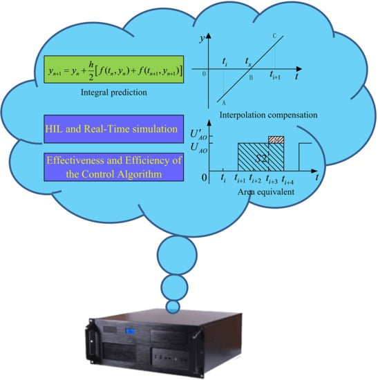
An integral prediction algorithm based on the implicit trapezoid method can accurately predict the value of the modulation wave of the next step and solve the switch delay in a fixed-step real-time simulation by a linear interpolation algorithm. Relying on the algorithm, the moment when the switch acts between the sampling points of simulation steps can be accurately determined to offer favorable conditions for the correction of output voltage from the converter.

(2)

In this paper, a S-function-based PWM generator modeling and Simulink-function-based insulated gate bipolar transistor (IGBT) modeling are proposed. The PWM generator mathematical model can output not only normal PWM signals but also time variables of pulse indication signals and switch action, while an IGBT mathematical model can correct the output signals if and when necessary.

(3)

In this paper, a control algorithm for the output voltage correction of converter based on the area equivalent principle is proposed. The algorithm ensures the correctness and accuracy of the output voltage and current of converter via the accurate equivalent pulse from IGBT in each switching cycle.

This paper consists of following parts: Section 2 gives an introduction to the integral prediction algorithm, linear interpolation algorithm and multiple switching; Section 3 provides the modeling method of the PWM generator and the IGBT, and the computing method of three-phase converter’s voltage at the AC side and current of the DC bus; Section 4 introduces and analyzes the output voltage correction algorithm proposed in this paper in details; Section 5 offers and discusses the simulation results of an AC-DC-AC converter at varying conditions; conclusions are given in Section 6.

2. Interpolation Prediction Algorithm

2.1. Integral Prediction

To ascertain the moment when the modulation wave and the carrier wave intersect, the correlations between the modulation wave and the carrier wave at the present moment and at the sampling point of the next step need to be understood. The integral prediction method is used in this paper to predict the next step of the modulation wave.

The numerical integral method has been extensively applied in the transient simulation of power electronics. To use this method, consideration shall be given to its convergence and stability, namely truncation error attenuation is guaranteed at any simulation step. The implicit trapezoid method is chosen to predict the modulation wave of the next step, and its integral equation is as follows [23]:

$$y_{n+1}=y_n+\frac{h}{2}\left[f(t_n,y_n)+f(t_{n+1},y_{n+1})\right]$$

(1)

where t_n = n∗h, h is the simulation step size, y_n is the sampled value at time t_n, y_n+1 is the sampled value at time t_n+1, and f(t_n,y_n) is a given function.

The implicit trapezoid method is used widely due to its simplicity, stability, high accuracy and adaptability to the stiff equation [23,24]. Equation (1) predicts the integral of modulation wave in a step (i.e., predicting the y_n+1 of the next step at t_n+1 by the y_n at t_n). The predicted value is compared to the one a step ahead. The prediction results are comparably ideal.

2.2. Interpolation Algorithm

Given the significant action delay of the PWM signal during large step simulation, to improve simulation accuracy it is required that the fixed-step simulation algorithm can accurately consider the moment when the switch acts. An effective method is the linear interpolation algorithm in Figure 1, which is simple, rapid and effective. In this algorithm, the system characteristics of two adjacent switch actions are assumed to fit by a linear relationship. The carrier frequency of power electronics devices is considered linear in a switch cycle as it is generally far higher than that of the modulation wave. Therefore, the linear interpolation algorithm is more appropriate [25,26,27].

To accurately predict the moment when the modulation wave and the carrier wave intersect, the difference between the two is studied. The intersection point of the modulation wave and the carrier wave corresponds to the zero-crossing point of their difference. Assuming that the modulation wave is greater than the carrier wave is logically true, and the modulation wave is smaller than the carrier wave is logically false, logical truth values as specified in

Table 1. The modulation wave and carrier logic relationship.

Correspondence	Logical Value
ur > uc	1 (True)
ur < uc	0 (False)

are obtained.

In Table 1: u_r is the modulated wave, u_c is the carrier wave.

If both are logically true or false, the relationships between the modulation wave and the carrier wave at the present sampling point and the sampling point of the next step can be defined as logical XNOR, otherwise logically XOR. In the case of logical XNOR, the modulation wave and the carrier wave do not intersect in the next step at the current moment. Otherwise, there is an intersection point in the next step, and the time of intersection shall be calculated.

As shown in Figure 1, the linear section ABC represents the difference curve of the modulation wave and the carrier wave, while t_i and t_i+1 are fixed-step sampling points. t_i = i∗T_s and t_i+1 = (i+1)∗T_s, where T_s is the simulation step and i = 1, 2, 3… A is the sampling point at the current moment, C is the sampling point at the next step moment, and B is the zero-crossing point of the linear section ABC, namely, the intersection point of the modulation wave and the carrier wave. Given the zero-crossing moment of point B is t_x, the following equation is obtained according to the principle of similar right triangles:

$$\frac{y_{i+1}-y_i}{t_{i+1}-t_i}=\frac{y_i}{t_x-t_i}$$

(2)

then:

$$t_x=t_i+\frac{y_i}{y_{i+1}-y_i}{T}_s$$

where y_i is the value at point A, y_i+1 is the value at point C, and T_s is the step. By Equation (2) the intersection time of the modulation wave and the carrier wave is obtained.

2.3. Solution of Multiple Switching

Multiple switching is defined as multiple switch actions in a simulation step at two or more moments. It is quite common in PWM converters and has a close connection with the switch frequency of power electronics devices, the system complication and the simulation step [28,29]. As the data in a simulation model can only be exchanged with other modules at the integral step, the generation process of PWM shall be done in the same submodule. In case of a group of 6-channel PWM, there may be 4 or more PWMs that take switch actions in a step. While 3/6 channels are negative to the other 3 channels, only the situation when two or three groups of switches act at the same time is studied.

At the time of the integral step, integral prediction is used to determine whether the switching action of each PWM occurs. If there are two switching actions at the same time, then the switching time of one group is delayed by 1 ns to prevent the switch from missing. Reordering is performed based on the moments when switches act to realize multiple switching.

3. Converter Modeling

3.1. PWM Generator Modeling

As noted before, the implicit trapezoid method can be used to obtain the sampling value of the modulation wave at the next step, and the moment when the modulation wave and the carrier wave intersect is known by logic judgment and the interpolation algorithm. In the following, an analysis will be conducted to understand how to use these variables in the mathematical modeling of a PWM generator. As shown in Figure 2, t_i, t_i+1, t_i+2, t_i+3 and t_i+4 represent the fixed-step sampling points. At each sampling point, in addition to sampling the modulation wave and carrier wave signal at the current moment, the PWM generator will judge the logic relationship between them at the present and the next moments. If the relationship is logical XOR, the logic level of pulse width indication signal will be changed; otherwise, it remains the same.

In Figure 2, Figure 2a indicates the waveforms of modulation wave (u_r) and carrier wave (u_c); the waveforms of PWM signals and PWM’ (pulse width indication signal) are shown in Figure 2b,c, respectively; Figure 2d shows the time when the modulation wave intersects with the carrier wave. In the following, the waveforms of sampling points in a cycle of carrier wave as shown in Figure 2 are analyzed:

(1)

Fixed-step sampling point t_i: sampling the logic relationship between the modulation wave and the carrier wave is known as false (u_r < u_c) at the current step and true (u_r > u_c) at the next step. Therefore, the modulation wave and the carrier wave are expected to intersect in a step from t_i to t_i+1, and the PWM signal at the intersection changes from low level to high level. Therefore, at the present moment, PWM’, the pulse indication signal, is changed from low level to high level, and the time corresponding to t_x is recorded as t_x(i).

(2)

Fixed-step sampling point t_i+1: the logic relationship between t_i+1 and t_i+2 is judged as XNOR by the method used in (1). Accordingly, the pulse indication signal remains at the high level as before. As the modulation wave intersects with the carrier wave in the previous step (between t_i and t_i+1), the PWM signal changes from low level to high level here.

(3)

Fixed-step sampling point t_i+2: the logic relationship between t_i+2 and t_i+3 is judged as XNOR. Accordingly, the pulse indication signal remains at the high level as before while the PWM signal does not change.

(4)

Fixed-step sampling point t_i+3: the logic relationship between t_i+2 and t_i+3 is judged as XOR. Accordingly, the pulse indication signal changes from high level to low level, and the time when the carrier wave intersects with the modulation wave is calculated and recorded as t_x(i+3). The PWM signal remains unchanged.

(5)

Fixed-step sampling point t_i+4: the logic relationship between t_i+3 and t_i+4 is judged as XOR. Accordingly, the pulse indication signal PWM’ changes from low level to high level again, and the time corresponding to t_x is recorded. As the modulation wave intersects with the carrier wave in the previous step (between t_i+3 and t_i+4), the PWM signal changes from high level to low level.

By analyzing the waveforms at each fixed-step sampling point in Figure 2, the following conclusions are drawn:

(a)

If at the present and the next-step sampling points, the logic relationship between the modulation wave and the carrier wave is XOR, the logic level of the pulse width indication signal shall change, and the time when they intersect shall be recorded. Otherwise, neither the logic level of the pulse width indication signal shall be changed, nor shall the time of intersection be recorded.

(b)

If the carrier wave intersects with the modulation wave between the present and the previous-step sampling points, the logic level of the PWM signals shall change; otherwise, it remains the same.

(c)

The pulse indication signal PWM’ is as wide as the PWM, but acts at 1 step in advance, creating conditions for correcting IGBT output voltage later.

(d)

The t_x at the rising/falling edge of the pulse indication signal PWM’ is recorded as the initial/final value, and their difference is expressed as $\mathsf{\Delta }\mathrm{t}=t_x(i+3)-t_x(i)$.

(e)

As the PWM signal changes only at the fixed-step sampling point, a delay is expected as compared to the actual time when the modulation wave and the carrier wave intersect. The time difference ∆t calculated based on the pulse indication signal PWM’ accurately represent the pulse width of the PWM signal in a switching cycle.

3.2. IGBT Mathematical Modeling

As a voltage-based power device extensively used in power electronics converters, IGBT controls the turn-on and turn-off through the gate voltage signal and is inversely parallel to fly-wheel diodes to prevent current breakdown due to sudden changes in inductive load current. Therefore, the combination of one-circuit IGBT, internal resistance, internal induction and fly-wheel diodes is equivalent to the series circuit in Figure 3 [30,31].

In Figure 3, the gate G, the collector C and the emitter E of IGBT are connected to the control signal, the positive and negative terminals of voltage respectively for mathematical modeling. By neglecting the conduction loss and switching loss of IGBT and its antiparallel diode, the equation to calculate the phase voltage of converter modeled based on IGBT/DIODES can be simplified as follows:

$$\{\begin{array}{l}{U}_{jO}={\displaystyle \sum _k{U}_{CEk}}\\ U_{CEk}=!G\times (U_F+U_L+U_R)\end{array}$$

(3)

where: U_jO is the voltage to the midpoint of the DC voltage (j = A, B, C); U_CEk is the voltage between the collector and the emitter of the IGBT, k = 1, 2; and 1 represents the upper arm and 2 represents the lower arm. !G is contrary to the gate control signal and values 1 or 0; U_L and U_R represent the voltages at both ends of the internal induction and internal resistance, respectively; while U_F is the simulated external voltage.

3.3. Calculation of Phase Voltage

The output voltage from the IGBT model is a numerical signal corresponding to the midpoint of DC bus. The phase voltage calculation equation can be expressed as:

$$U_{jN}=U_{jO}-\frac{1}{3}{\displaystyle \sum _j{U}_{jO}}$$

(4)

where: U_jN is the phase voltage (j = A, B, C), and U_jO is the voltage corresponding to the midpoint of DC. By Equation (4), the numerical signal of the three-phase voltage of the converter is calculated and transferred to an electrical signal through the controlled voltage source, realizing the connection with the electronics in the Simulink for joint simulation.

3.4. Calculation of DC Bus Current

Power loss is generally neglected in power electronics simulation. According to the principle of conservation of energy, the input/output power at the DC side is equal to the output/input power at the AC side of the converter, namely:

$$U_{dc}\times I_{dc}={\displaystyle \sum _j(U_{jN}\times I_{jN})}$$

(5)

where: U_dc and I_dc represent the voltage and current of the DC bus, respectively; U_jN and I_jN represent the phase voltage and phase current, respectively. According to Equation (5), the current of DC bus is calculated. As the signal is numerical, it shall be converted to an electrical signal by the controlled current source to connect with the power module in Simulink.

4. Correction Compensation Algorithm

When the PWM signal in Figure 2b is used to control the IGBT for turn-on and turn-off, the output voltage is inaccurate as it contains many non-characteristic harmonics, and therefore requires necessary correction. In the following, the area equivalence principle is introduced by taking the A-phase upper-tube IGBT of a three-phase converter as an example. The output voltage amplitude of IGBT is U_AO (U_AO = U_dc/2).

Figure 4a shows the waveforms of the modulation wave and the carrier wave. Ideally, it is expected to control the IGBT actions at the intersection to output the voltage waveform as shown in Figure 4b. However, IGBT only acts at the integral-step sampling point, and the actually output voltage waveform is shown in Figure 4c. Evidently, there is an error as the pulse area $S_1\ne S_2$.

In Figure 4d, the numerical model-based IGBT output voltage is corrected in the last step of the pulse width by the area equivalent principle. The area equivalent equation is as follows:

$$U_{AO}\cdot \mathsf{\Delta }t=U_{AO}\cdot (t_{i+3}-t_{i+1})+{U^{\prime }}_{AO}\cdot T_s$$

(6)

According to Equation (6):

$$\{\begin{array}{l}{U^{\prime }}_{AO}=\frac{U_{AO}\cdot \left[\mathsf{\Delta }t-(t_{i+3}-t_{i+1})\right]}{T_s}\\ \mathsf{\Delta }s=({U^{\prime }}_{AO}-U_{AO})\cdot T_s\end{array}$$

(7)

where: $\mathsf{\Delta }\mathrm{t}=t_x(i+3)-t_x(i)$ is the actual pulse width between two intersection points of the modulation wave and the carrier wave; $U_{AO}$ and ${U^{\prime }}_{AO}$ are the output voltage amplitudes when IGBT is normal and at the last step, respectively; $\mathsf{\Delta }s$ is the correction, which may be positive or negative.

At t_i+3, the actual pulse width $\mathsf{\Delta }\mathrm{t}$ is calculated according to the pulse indication signal in Figure 4c; when the IGBT is still outputting, the output voltage amplitude from the IGBT numerical model in the last step can be corrected necessarily to change it from $U_{AO}$ to ${U^{\prime }}_{AO}$, so that the area $S_1=S_2+\mathsf{\Delta }s$. Therefore, the equivalency between the output volume of the IGBT and the actual pulse in a switching cycle is guaranteed.

For other IGBT mathematical models of the three-phase converter, similar methods also apply.

5. Case Analysis

According to the relationship between the actual response time and the system simulation time, the simulation of a power system may be offline or real-time online. In offline simulation, the operation of actual objects is simulated in software installed on the computer, while in the real-time online simulation, the real-time simulator is used to simulate the operation of an actual object in real conditions, in which, the simulation clock is perfectly consistent with the real clock. Under the two conditions, the interpolation prediction algorithm is analyzed and verified.

5.1. Interpolation Algorithm-Based Case Analysis of Converter

To verify the correctness and effectiveness of PWM converters based on an integral prediction and interpolation algorithm under large-step simulation, MATLAB/Simulink software is used here for offline simulation. An AC-DC-AC converter model built by IGBT was used as a simulation example, as shown in Figure 5, and the parameters of the simulation example are listed in

Table 2. Simulation model parameters.

Project	Parameter
Step-down transformer capacity	50 kVA
Rectifier grid sideline voltage	400 V, 60 Hz
Inverter load sideline voltage	380 V, 50 Hz
DC bus voltage	750 V

. In this example, the power grid is a 25 kV/60 Hz alternating current, and the power is converted to a 380 V/50 Hz alternating current to supply load through step-down transformer and converter. The load power is 25 kW when the simulation begins and rises to 50 kW at 0.15 s when the breaker is closed.

By comparing, the simulation waveforms in Figure 6a,b, though the simulation step of the interpolation prediction model is 50 μs, its simulation result is consistent with the 5 μs standard model. According to the steady-state waveform, the simulation accuracy of the interpolation prediction model with step of 50 μs is exactly the same as a 5 μs standard model.

To verify the simulation accuracy of the interpolation prediction model, the A-phase current of the load is observed. Figure 7a is the waveform of load A-phase current obtained in a standard model with step of 5 μs and 50 μs, respectively. Figure 7b is the waveform of load A-phase current obtained in a standard model with step of 5 μs and in an interpolation prediction model with step of 50 μs, respectively. The current waveform at 5 μs is marked as blue, and the current waveform at 50 μs is marked as red.

According to the global waveform in Figure 7a, when the simulation step increases to 50 μs, the current waveform in the standard model fluctuates significantly and cannot overlap with the current waveform at 5 μs. When the load suddenly increases at 0.15 s, there is a significant error between the 50 μs current waveform (red) and the 5 μs current waveform (blue) according to the local transient process from 0.149 to 0.151 s, suggesting that the increase in step will amplify the delay in switch action when Simulink basic module is used for simulation, resulting in many non-characteristic harmonic waves.

According to the global waveform in Figure 7b, though the simulation step increases to 50 μs, the current waveform in the interpolation prediction model overlaps with the current waveform at 5 μs in the standard model. When the load suddenly increases at 0.15 s, there is an insignificant error between the 50 μs current waveform (red) and the 5 μs current waveform (blue) according to the local transient process from 0.149 to 0.151 s, showing basically the same simulation accuracy.

5.2. Analysis of PWM Effectiveness Based on Interpolation Prediction Model

To analyze the effectiveness of PWM based on the interpolation prediction model, the key lies in accurately restoring the harmonic waves. Here, the A-phase voltage at the converter load side is taken as the subject. The content of harmonic wave in the A-phase bridge arm voltage waveform at the 5 μs standard model and the 50 μs interpolation prediction model are compared. The FFT analysis results are shown in Figure 8.

Figure 8a shows the FFT analysis results of the load-side A phase in the detailed model of the converter built on the basis of Simulink basic modules at the step of 5 μs while Figure 8b represents the FFT analysis results of the load-side A-phase in the interpolation prediction model at the step of 50 μs. The area equivalent principle is adopted to calculate the phase voltage. Therefore, the output voltage waveform in this model varies from that of the 5 μs standard model.

The THD is 89.78% in Figure 8a and 92.90% in Figure 8b. Regardless of the slight difference, both show a generally basic tendency. By comparing the 5 μs detailed switch model to the 50 μs interpolation prediction model, the effectiveness of PWM in the 50 μs interpolation prediction model is verified.

5.3. Efficient Analysis Based on Interpolation Prediction Model

To verify whether the interpolation prediction model can improve simulation efficiency, a 1 s simulation test was performed with the 5 μs standard model and the 50 μs interpolation prediction model, and the time consuming data was checked in the Diagnostic Viewer of MATLAB, as shown in

Table 3. Model actual execution time.

Simulation Type	Step Length	The Simulation Time	The Actual Time Consumed
Standard model	5 μs	1 s	13.2 s
Interpolation prediction model	50 μs	1 s	4.5 s

.

According to the time consuming data of the simulation operation in Table 3, under the simulation conditions using the same device, the time consumed by the 50 μs interpolation model is significantly shorter and accounts for only about one third of the time consumed by a 5 μs detailed standard model. This is typically due to the increased model calculation times and therefore improved simulation efficiency by enlarging the simulation step. It also certifies the efficiency of the interpolation prediction model.

5.4. Real-Time Simulation Based on Interpolation Prediction Model

Figure 9a,b shows the voltage and current waveforms of the standard model and the interpolation prediction model on the real-time simulators, respectively. As the simulation step adopted in the real-time simulation is 50 μs, the waveforms of voltage and current in the standard model are disordered, while these in the interpolation prediction model are beyond comparison. Therefore, real-time simulation comparison further verifies the correctness and effectiveness of the interpolation prediction model, and also suggests that the interpolation prediction model could realize the simulation of a small-step model in a large-step real-time simulator.

6. Conclusions

This paper puts forward an interpolation-prediction-based PWM generator modeling method and an area-equivalent-based IGBT modeling method. Offline simulation and case analysis were performed in MATLAB/Simulink, and real-time simulation verification was performed in a real-time simulator. The following conclusions area drawn.

(1)

In the interpolation-prediction-based PWM generator modeling method, the switching point at any moment under the fixed-step simulation condition can be determined by one-time integral prediction and linear interpolation. The accuracy of the switching point can be equal to or even higher than a 5 μs standard model.

(2)

In the area-equivalent-based IGBT modeling method, the IGBT action process is processed for equivalence according to the predicted switching time points, so as to ensure the accuracy of output signals from the IGBT numerical model in each switching cycle, and realize the compatibility with the power modules in the Simulink by signal conversion through the controlled voltage source.

(3)

By case analysis, the effectiveness and efficiency of the control algorithm proposed in this paper are verified. The interpolation-prediction-based control algorithm effectively reduces the non-characteristic harmonic waves arising from switch delay, while the steadiness and transience are good. Due to the increase in simulation step, the operation efficiency of the model also significantly rises.

(4)

The modeling methods and control algorithm recommended in this paper apply not only to hardware in-loop simulation and real-time simulation platforms, but also to fixed-step electromagnetic transient simulation.

In conclusion, the modeling methods and control algorithm suggested in this paper realize the offline simulation and real-time online simulation at large steps, ensure the accuracy and efficiency of simulation, and play an active role in the simulation research of power electronics.

References

1. Li, B.; He, J.; Li, B. A review of the protection for the multi-terminal VSC-HVDC grid. Prot. Control Mod. Power Syst. 2019, 4, 1–11. [Google Scholar] [CrossRef]
2. Aleem, S.A.; Hussain, S.M.; Ustun, T.S. A Review of Strategies to Increase PV Penetration Level in Smart Grids. Energies 2020, 13, 636. [Google Scholar] [CrossRef] [Green Version]
3. Shu, D.; Xie, X.; Jiang, Q.; Hang, Q.; Zhang, C. A Novel Interfacing Technique for Distributed Hybrid Simulations Combining EMT and Transient Stability Models. IEEE Trans. Power Deliv. 2018, 33, 130–140. [Google Scholar] [CrossRef]
4. Albaidhani, H.; Kazimierczuk, M.K.; Reatti, A. Nonlinear Modeling and Voltage-Mode Control of DC-DC Boost Converter for CCM. In Proceedings of the 2018 IEEE International Symposium on Circuits and Systems, Florence, Italy, 27–30 May 2018; pp. 1–5. [Google Scholar]
5. Ivanovic, Z.R.; Adzic, E.M.; Vekic, M.S.; Grabic, S.; Celanovic, N.; Katic, V. HIL evaluation of power flow control strategies for energy storage connected to smart grid under unbalanced conditions. IEEE Trans. Power Electron. 2012, 27, 4699–4710. [Google Scholar] [CrossRef]
6. Zhang, J.; Xiong, G.; Meng, K.; Yu, P.; Yao, G.; Dong, Z. An improved probabilistic load flow simulation method considering correlated stochastic variables. Int. J. Electr. Power Energy Syst. 2019, 111, 260–268. [Google Scholar] [CrossRef]
7. Huang, Q.; Vittal, V. Application of Electromagnetic Transient-Transient Stability Hybrid Simulation to FIDVR Study. IEEE Trans. Power Syst. 2016, 31, 2634–2646. [Google Scholar] [CrossRef]
8. Sybille, G.; Lehuy, H. Digital Simulation of Power Systems and Power Electronics using the MATLAB/Simulink Power System Blockset. In Proceedings of the IEEE Power Engineering Society-Winter Meeting 2000 Special Technical Session, Singapore, 23–27 January 2000; pp. 2973–2982. [Google Scholar]
9. Faruque, M.O.; Dinavahi, V. Hardware-in-the-loop simulation of power electronic systems using adaptive discretization. IEEE Trans. Ind. Electron. 2010, 57, 1146–1158. [Google Scholar] [CrossRef]
10. Lauss, G.; Faruque, M.O.; Schoder, K.; Dufour, C.; Viehweider, A.; Langston, J. Characteristics and Design of Power Hardware-in-the-Loop Simulations for Electrical Power Systems. IEEE Trans. Ind. Electron. 2016, 63, 406–417. [Google Scholar] [CrossRef]
11. Carbone, R.; Rosa, F.D.; Langella, R.; Testa, A. A new approach for the computation of harmonics and interharmonics produced by line-commutated AC/DC/AC converters. IEEE Trans. Power Deliv. 2005, 20, 2227–2234. [Google Scholar] [CrossRef]
12. Bilik, P.; Zidek, J.; Kus, V.; Josefova, T. Harmonic Currents of Semiconductor Pulse Switching Converters. Energy Power Eng. 2013, 5, 1120–1125. [Google Scholar] [CrossRef]
13. Wang, Q.; Wu, J.; Gao, J.; Wang, J.; Li, C.; Wang, J.J.; Zhou, N. Frequency-domain harmonic modeling and analysis for 12-pulse series-connected rectifier under unbalanced supply voltage. Electr. Power Syst. Res. 2018, 162, 23–36. [Google Scholar] [CrossRef]
14. Tant, J.; Driesen, J. Accurate second-order interpolation for power electronic circuit simulation. In Proceedings of the 18th IEEE Workshop on Control and Modeling for Power Electronics, Stanford, CA, USA, 9–12 July 2017; pp. 1–8. [Google Scholar]
15. Strunz, K. Flexible numerical integration for efficient representation of switching in real time electromagnetic transients Simulation. IEEE Trans. Power Deliv. 2004, 19, 1276–1283. [Google Scholar] [CrossRef]
16. Shu, D.; Xie, X.; Jiang, Q.; Guo, G.; Wang, K. A Multirate EMT Co-Simulation of Large AC and MMC-Based MTDC Systems. IEEE Trans. Power Syst. 2018, 33, 1252–1263. [Google Scholar] [CrossRef]
17. Faruque, M.O.; Strasser, T.; Lauss, G.; Jalili-Marandi, V.; Forsyth, P.; Dufour, C.; Dinavahi, V.; Monti, A.; Kotsampopoulos, P.; Martinez, J.A.; et al. Real-time simulation technologies for power systems design, testing, and analysis. IEEE Power Energy Technol. Syst. 2015, 2, 63–73. [Google Scholar] [CrossRef]
18. Liu, X.; Cramer, A.M.; Pan, F. Generalized average method for time-invariant modeling of inverters. IEEE Trans. Circuits Syst. 2017, 64, 740–751. [Google Scholar] [CrossRef]
19. Peralta, J.; Saad, H.; Dennetiere, S.; Mahseredjian, J.; Nguefeu, S. Detailed and Averaged Models for a 401-Level MMC-HVDC System. IEEE Trans. Power Deliv. 2012, 27, 1501–1508. [Google Scholar] [CrossRef]
20. dSPACE Inc. dSPACE User Guide-Implementation Guide; dSPACE Inc.: Paderborn, Germany, 2005. [Google Scholar]
21. OPAL-RT. RT-LAB 8.2.1 User’s Manual; Opal-RT Technologies Incorporation: Montreal, QC, Canada, 2008. [Google Scholar]
22. Olimpo, A.; Acha, E. Modeling and Analysis of Custom Power Systems by PSCAD/EMTDC. IEEE Power Energy Mag. 2001, 17, 266–272. [Google Scholar]
23. Pekarek, S.D.; Wasynczuk, O.; Walters, E.; Jatskevich, J.; Lucas, C.E.; Wu, N.; Lamm, P. An efficient multirate Simulation technique for power-electronic-based systems. IEEE Trans. Power Syst. 2004, 19, 399–409. [Google Scholar] [CrossRef]
24. Noda, T.; Kikuma, T.; Yonezawa, R. Supplementary techniques for 2S-DIRK-based EMT simulations. Electr. Power Syst. Res. 2014, 115, 87–93. [Google Scholar] [CrossRef]
25. Zou, M.; Mahseredjian, J.; Joos, G.; Delourme, B.; Gerinlajoie, L. Interpolation and reinitialization in time-domain simulation of power electronic circuits. Electr. Power Syst. Res. 2006, 76, 688–694. [Google Scholar] [CrossRef]
26. Kuffel, P.; Kent, K.; Irwin, G. The implementation and effectiveness of linear interpolation within digital simulation. Electr. Power Energy Syst. 1997, 19, 221–227. [Google Scholar] [CrossRef]
27. Tant, J.; Driesen, J. On the Numerical Accuracy of Electromagnetic Transient Simulation with Power Electronics. IEEE Trans. Power Deliv. 2018, 33, 2492–2501. [Google Scholar] [CrossRef]
28. Faruque, M.O.; Dinavahi, V.; Xu, W. Algorithms for the accounting of multiple switching events in digital simulation of power-electronic systems. IEEE Trans. Power Deliv. 2005, 20, 1157–1167. [Google Scholar] [CrossRef]
29. Liang, G.; Song, C.; Wen, S. Algorithms for the Accounting of Multiple Switching Events in Real-Time Simulation of Distributed Power. In Proceedings of the 2019 IEEE 10th International Symposium on Power Electronics for Distributed Generation Systems (PEDG), Xi’an, China, 3–6 June 2019; pp. 237–241. [Google Scholar]
30. Hao, B.; Chen, L.; Akshay, K.R.; Damien, P.; Fei, G. An FPGA-Based IGBT Behavioral Model with High Transient Resolution for Real-Time Simulation of Power Electronic Circuits. IEEE Trans. Power Electron. 2019, 66, 6581–6591. [Google Scholar]
31. Ji, S.; Lu, T.; Zhao, Z.; Yuan, L. Modelling of High Voltage IGBT with Easy Parameter Extraction. In Proceedings of the 7th International Power Electronics and Motion Control Conference (IPEMC 2012), Harbin, China, 2–5 June 2012; pp. 1511–1515. [Google Scholar]
Figure 1. Pulse-width modulating (PWM) switching point determination.
Energies 13 03069 g001
Figure 2. Bipolar PWM control mode waveform: (a) carrier and modulated waves; (b) actual PWM signal; (c) indicator signal PWM; (d) switching action time.
Energies 13 03069 g002
Figure 3. The insulated gate bipolar transistor (IGBT) equivalent model.
Energies 13 03069 g003
Figure 4. Schematic diagram of area equivalent correction: (a) carrier and modulated waves; (b) expect pulse; (c) the actual pulse; (d) corrected pulse.
Energies 13 03069 g004
Figure 5. AC-DC-AC Converter simulation model.
Energies 13 03069 g005
Figure 6. Comparison of standard model and interpolation prediction model: (a) 5 μs standard model grid side waveform; (b) 50 μs interpolation prediction model power grid side waveform.
Energies 13 03069 g006
Figure 7. A-phase current comparison on the load side: (a) comparison of A-phase current on load side of 5 μs and 50 μs standard models; (b) comparison of A-phase current on load side of 5 μs standard model and 50 μs interpolation prediction model.
Energies 13 03069 g007
Figure 8. FFT analysis of A-phase voltage of load side: (a) 5 μs standard model; (b) 50 μs interpolation prediction model.
Energies 13 03069 g008
Figure 9. Real-time simulation comparison: (a) 50 μs real-time simulation of standard model; (b) 50 μs real-time simulation of interpolation prediction model.
Energies 13 03069 g009aEnergies 13 03069 g009b