Efficient Unbalanced Three-Phase Network Modelling for Optimal PV Inverter Control

Abstract

High penetration levels of renewable energy generation in the distribution network require voltage regulation to avoid excessive voltage at generating nodes. To effectively control the network and optimize network hosting capacity, the distribution system operator must have an efficient model for power flow analysis. This paper presents the formulas and steps to express the power flow analysis equations of an unbalanced 3-phase network in matrix form suited to programmed solutions. A benchmark MATLAB/Simulink network with unbalanced distribution lines, photovoltaic inverters, and loads is built to verify the matrix model. To demonstrate the application of the model, the control of reverse energy flow from the photovoltaic inverters to keep the voltage in the network below the regulated level is simulated. Two decentralized control algorithms are applied in the network, including an on/off and a multi-objective constrained optimization controller. The detailed construction of the optimization problem for the 3-phase network in matrix form, which is consistent with the power flow calculation, is described. Simulation with the control methods over a day shows that the total active power of the on/off and optimized controllers deliver 41.92% and 99.39% of the available solar power, respectively, while maintaining the network node voltages within limits.

1. Introduction

The increasing penetration of photovoltaic (PV) distributed generation (DG) in the low voltage (LV) distribution system raises difficulties for the distribution system operator (DSO) in maintaining voltage stability. Reverse power flow from PV sources causes a rise in node voltage and this is a key factor limiting the PV hosting capacity of a network [1]. The introduction of emerging smart-grid technology with advanced system control should enable the widespread integration of renewable energies. The smart grid with smart meters and high-speed broadband communication allows for the use of decentralized controls to address these distribution system problems [2,3]. There are different methods to determine the network voltage by Gauss–Seidel [4], Newton–Raphson [4,5,6,7,8,9], Fast Decoupled Load Flow (FDLF), Backward/Forward sweep power flow (BFS) [10,11,12] and a linear approach [13,14,15]. In this paper, the Newton–Raphson method is selected for its robustness and quadratic convergence [16,17]. In the Newton–Raphson method, the components can be expressed in three coordinates of polar, Cartesian and complex forms for both the power and current mismatch formulations [6].

The power flow analysis problem is developed mainly for constant power P-Q buses with one constant voltage swing bus. The power flow is also applied for constant power-voltage P-V buses [18] and different load models, such as constant impedance (Z), constant current (I) [8] and polynomial or combined constant impedance (Z), constant current (I) and constant power (P) ZIP loads [19]. There are power flow investigations of the transformer tap change [20], the FACTS (Flexible AC Transmission System) controllers, including IPFC (Interline Power Flow Controller) [21], UPFC (Unified Power Flow Controller) [22,23,24], STATCOM (Static Synchronous Compensator) [18,20]. These power flow calculations cover devices and components in the single-phase and balanced 3-phase distribution network but an extension is needed for the unbalanced 3-phase network.

In practice, the loads and DG in the distribution network are not all equally connected between three phases and the components of resistance and inductance of the 3-phase distribution conductors are not the same. Therefore, in the case of unbalanced 3-phase [25,26,27], there is the need to formulate an unbalanced 3-phase power flow analysis for the network with different voltage magnitude in each phase. Similar to the balanced network, there are studies to address the unbalanced 3-phase, including P-V buses [9,14,15] and ZIP load [14,15]. The effect of transformers and loads with different wye and delta connections is considered in the 3-phase network [14,28]. The Newton–Raphson power flow calculation methods are also presented in an unbalanced network as in [7,9]. These studies show the power flow calculation of the network and the steady-state results of the network analysis. The next step is the application of the power flow calculation into a network with a time-scale and control strategies.

Some previous research applied the power flow for the optimization of the PV inverters in the network [29], including the single-objective [30] and multi-objective optimization [31,32,33]. However, these applications are limited to the power calculation of the unbalanced 3-phase network. In this paper, the unbalanced power flow analysis is applied to the distribution network integrating residential loads and PV inverters for the optimization in matrix form. The control algorithms applied in this work are based on a decentralized control where all PV inverters in the network are controllable with the reactive power support to regulate the bus voltage and power factor within the prescribed limits.

In this paper, the formulas are all presented in matrix form which shows advantages in coding and presentation. This is similar to using the complex form whose amplitude and angle or the real and imaginary parts are presented in a single complex number. There are previous efforts to reduce the complexity of the formulas and calculations of power flow in a different presentation [34] and in complex form [6,35], which cut down the dimensions of Jacobian, voltage and power matrices by half. Below are the typical formulas of Newton–Raphson current mismatch in a specific phase $\mathrm{p}$ at bus $\mathrm{I}$, where $\mathrm{p}$ is presented for phase a, b and c [7].

$$\mathsf{\Delta }{\mathrm{I}}_{\mathrm{r}\left(\mathrm{i}\right)}^{\mathrm{p}}=\frac{{\mathrm{P}}_{\mathrm{sh}\left(\mathrm{i}\right)}^{\mathrm{p}}\cos {\mathsf{\delta }}_{\mathrm{i}}^{\mathrm{p}}+{\mathrm{Q}}_{\mathrm{sh}\left(\mathrm{i}\right)}^{\mathrm{p}}\sin {\mathsf{\delta }}_{\mathrm{i}}^{\mathrm{p}}}{\left|{\mathrm{V}}_{\mathrm{i}}^{\mathrm{p}}\right|}-{{\displaystyle \sum }}_{\mathrm{k}=1}^{\mathrm{N}}{{\displaystyle \sum }}_{\mathrm{q}=\mathrm{a},\mathrm{b},\mathrm{c}}\left|{\mathrm{V}}_{\mathrm{k}}^{\mathrm{q}}\right|\left({\mathrm{G}}_{\mathrm{ik}}^{\mathrm{pq}}\cos {\mathsf{\delta }}_{\mathrm{k}}^{\mathrm{p}}-{\mathrm{B}}_{\mathrm{ik}}^{\mathrm{pq}}\sin {\mathsf{\delta }}_{\mathrm{k}}^{\mathrm{p}}\right)$$

(1)

$$\frac{\partial \mathsf{\Delta }{\mathrm{I}}_{\mathrm{r}\left(\mathrm{i}\right)}^{\mathrm{p}}}{\partial {\mathsf{\delta }}_{\mathrm{i}}^{\mathrm{p}}}=-\frac{{\mathrm{P}}_{\mathrm{sh}\left(\mathrm{i}\right)}^{\mathrm{p}}\sin {\mathsf{\delta }}_{\mathrm{i}}^{\mathrm{p}}-{\mathrm{Q}}_{\mathrm{sh}\left(\mathrm{i}\right)}^{\mathrm{p}}\cos {\mathsf{\delta }}_{\mathrm{i}}^{\mathrm{p}}}{\left|{\mathrm{V}}_{\mathrm{i}}^{\mathrm{p}}\right|}+\left|{\mathrm{V}}_{\mathrm{i}}^{\mathrm{p}}\right|\left({\mathrm{G}}_{\mathrm{ii}}^{\mathrm{pp}}\sin {\mathsf{\delta }}_{\mathrm{i}}^{\mathrm{p}}+{\mathrm{B}}_{\mathrm{ii}}^{\mathrm{pp}}\cos {\mathsf{\delta }}_{\mathrm{i}}^{\mathrm{p}}\right)$$

(2)

The presentation of phase in an index listed format as in the above equations is also in [9,15]. The matrix form of complete power flow formulas and the optimization construction is presented in Section 2 and Section 3. The 3-phase matrix presentation shows the same goal to the research of complex power flow analysis. Some papers represent the power flow equation in matrix form [13,14]; however, they are applied for the linear approach and the optimization control is not presented. This paper put an effort to present all elements in the 3-phase matrices and treat them in formulas as the balanced system and reduce the amount of formula by a third by combining the three specific phases into a matrix. This presentation also avoids the confusion of switching between the scalar and matrix forms in the same formula. Besides, this reduces the mistakes or errors in the programming and reduces the number of coding loops. After the calculation of the power flow of the unbalanced 3-phase network, the optimization control is applied to the network and the construction of the control is also presented in the matrix form which is consistent with the power flow calculation.

This paper includes two main parts. The first part develops a process for network description and power flow analysis in a matrix form as seen in Section 2. The process is applied to describe a benchmark 20-bus distribution network model in Section 3. Power flow analysis is conducted with the model under a measured irradiation profile and this results in overvoltage conditions with node voltages as high 1.3 pu. The second part, Section 4 and Section 5, employs the same network model and applies two different decentralized control methods to eliminate overvoltage conditions. The decentralized algorithms use smart grid communication to provide knowledge of the load and potential PV power at each node to a central computer where the algorithm employs power flow analysis to identify overvoltage conditions and modifies the PV power output to maintain the voltage within limits. Section 4 describes the two control algorithms: a simple overvoltage control and a multi-objective optimization algorithm. The detailed construction of the constrained optimization problem in matrix form, consistent with the power flow calculation, is described. Section 5 presents a comparison of the performance results of the control methods. The discussion of the contribution and comparison to other research as well as the limit scope of this paper is presented in Section 6.

2. Power Flow Matrix Formation of an Unbalanced 3-Phase Network

In a network of $\mathrm{N}$ buses with known distribution line parameters and scheduled power of $P_{\mathrm{sh}}$ and $Q_{\mathrm{sh}}$, the voltage magnitude $\left|V\right|$ and voltage angle $\delta$ can be calculated using the Newton–Raphson method [4,5] with the current-mismatch function $\mathbf{\Delta }I$ in the polar-coordinate format [6,7].

The Newton–Raphson method uses an iteration of calculations to find the results. The initial values of angle and magnitude of all buses are set at ${\delta }^{\left(0\right)}$ and ${\left|V\right|}^{\left(0\right)}$ as in (3). In Equation (4), the next estimates of ${\delta }^{\left(\mathrm{h}+1\right)}$ and ${\left|V\right|}^{\left(\mathrm{h}+1\right)}$ are computed by adding the previous values to the differences of $\mathsf{\Delta }\delta$ and $\mathsf{\Delta }\left|V\right|$, which are determined in (5).

$${\delta }_{\mathrm{i}}^{\left(0\right)}=\left[\begin{array}{c}0\\ -2\mathsf{\pi }/3\\ 2\mathsf{\pi }/3\end{array}\right]{\left|V_{\mathrm{i}}\right|}^{\left(0\right)}=\left[\begin{array}{c}1\\ 1\\ 1\end{array}\right]\left(\mathrm{pu}\right)$$

(3)

$${\left|V\right|}^{\left(\mathrm{h}+1\right)}={\left|V\right|}^{\left(\mathrm{h}\right)}+\mathsf{\Delta }\left|V\right|\mathrm{and}{\delta }^{\left(\mathrm{h}+1\right)}={\delta }^{\left(\mathrm{h}\right)}+\mathsf{\Delta }\delta$$

(4)

Bus 1 is the swing bus, the voltage magnitude $\left|V_1\right|$ and angle ${\delta }_1$ of which are known. The values of the remaining ($\mathrm{N}-1$) buses need to be determined using the Jacobian matrices, $J_1$ to $J_4$, that calculate the partial derivatives of current with respect to voltage angles and magnitudes.

$$\begin{array}{c}-\left[\begin{array}{cc}{J}_1& J_2\\ J_3& J_4\end{array}\right]\left[\begin{array}{c}\mathsf{\Delta }\delta \\ \mathsf{\Delta }\left|V\right|\end{array}\right]=\left[\begin{array}{c}\mathsf{\Delta }{I}_{\mathrm{r}}\\ \mathsf{\Delta }{I}_{\mathrm{m}}\end{array}\right]\\ \mathsf{\Delta }\delta =\left[\begin{array}{c}\mathsf{\Delta }{\delta }_2\\ ⋮\\ \mathsf{\Delta }{\delta }_{\mathrm{N}}\end{array}\right],\mathsf{\Delta }\left|V\right|=\left[\begin{array}{c}\mathsf{\Delta }\left|V_2\right|\\ ⋮\\ \mathsf{\Delta }\left|V_{\mathrm{N}}\right|\end{array}\right],\mathsf{\Delta }I=\mathsf{\Delta }{I}_{\mathrm{r}}+\mathrm{j}\mathsf{\Delta }{I}_{\mathrm{m}}=\left[\begin{array}{c}\mathsf{\Delta }{I}_2\\ ⋮\\ \mathsf{\Delta }{I}_{\mathrm{N}}\end{array}\right],J=\left[\begin{array}{ccc}{J}_{11}& \cdots & J_{1\left(\mathrm{N}-1\right)}\\ ⋮& \ddots & ⋮\\ J_{\left(\mathrm{N}-1\right)1}& \cdots & J_{\left(\mathrm{N}-1\right)\left(\mathrm{N}-1\right)}\end{array}\right]\end{array}$$

(5)

Each element inside matrices $\mathsf{\Delta }\delta$, $\mathsf{\Delta }\left|V\right|$ and $\mathsf{\Delta }I$ is a 3 × 1 matrix. The matrices $J_1$ to $J_4$ have the same dimension as $J$, and each element of $J$ is a matrix whose dimension is 3 × 3. The formulas for all elements of the matrices in (5) are presented in

Table 1. Elements of Jacobian and current-mismatch matrices.

$\mathsf{\Delta }I=\mathsf{\Delta }{I}_{\mathrm{r}}+\mathrm{j}\mathsf{\Delta }{I}_{\mathrm{m}}$ $\mathrm{i}=2:\mathrm{N}$	$\mathsf{\Delta }{I}_{\mathrm{r}\left(\mathrm{i}\right)}=\left(P_{\mathrm{sh}\left(\mathrm{i}\right)}\odot \cos {\delta }_{\mathrm{i}}+Q_{\mathrm{sh}\left(\mathrm{i}\right)}\odot \sin {\delta }_{\mathrm{i}}\right)\oslash \left|V_{\mathrm{i}}\right|$ $-{{\displaystyle \sum }}_{\mathrm{k}=1}^{\mathrm{N}}\left(G_{\mathrm{ik}}\mathrm{diag}\left(\cos {\delta }_{\mathrm{k}}\right)-B_{\mathrm{ik}}\mathrm{diag}\left(\sin {\delta }_{\mathrm{k}}\right)\right)\mathrm{diag}\left(\left|V_{\mathrm{k}}\right|\right){\left[111\right]}^{\mathrm{T}}$
	$\mathsf{\Delta }{I}_{\mathrm{m}\left(\mathrm{i}\right)}=\left(P_{\mathrm{sh}\left(\mathrm{i}\right)}\odot \sin {\delta }_{\mathrm{i}}-Q_{\mathrm{sh}\left(\mathrm{i}\right)}\odot \cos {\delta }_{\mathrm{i}}\right)\oslash \left|V_{\mathrm{i}}\right|$ $-{\displaystyle \sum }_{\mathrm{k}=1}^{\mathrm{N}}\left(G_{\mathrm{ik}}\mathrm{diag}\left(\sin {\delta }_{\mathrm{k}}\right)+B_{\mathrm{ik}}\mathrm{diag}\left(\cos {\delta }_{\mathrm{k}}\right)\right)\mathrm{diag}\left(\left|V_{\mathrm{k}}\right|\right){\left[111\right]}^{\mathrm{T}}$
Diagonal $\mathrm{i}=2:\mathrm{N}$	$J_{1\left(\mathrm{i}-1,\mathrm{i}-1\right)}=-{\left(\left(\left(P_{\mathrm{sh}\left(\mathrm{i}\right)}\odot \sin {\delta }_{\mathrm{i}}-Q_{\mathrm{sh}\left(\mathrm{i}\right)}\odot \cos {\delta }_{\mathrm{i}}\right)\oslash \left|V_{\mathrm{i}}\right|\right)\left[111\right]\right)}^{\mathrm{T}}+\left(G_{\mathrm{ii}}\mathrm{diag}\left(\sin {\delta }_{\mathrm{i}}\right)+B_{\mathrm{ii}}\mathrm{diag}\left(\cos {\delta }_{\mathrm{i}}\right)\right)\mathrm{diag}\left(\left|V_{\mathrm{i}}\right|\right)$
	$J_{3\left(\mathrm{i}-1,\mathrm{i}-1\right)}=+{\left(\left(\left(P_{\mathrm{sh}\left(\mathrm{i}\right)}\odot \sin {\delta }_{\mathrm{i}}+Q_{\mathrm{sh}\left(\mathrm{i}\right)}\odot \cos {\delta }_{\mathrm{i}}\right)\oslash \left|V_{\mathrm{i}}\right|\right)\left[111\right]\right)}^{\mathrm{T}}-\left(G_{\mathrm{ii}}\mathrm{diag}\left(\sin {\delta }_{\mathrm{i}}\right)-B_{\mathrm{ii}}\mathrm{diag}\left(\cos {\delta }_{\mathrm{i}}\right)\right)\mathrm{diag}\left(\left|V_{\mathrm{i}}\right|\right)$
	$J_{2\left(\mathrm{i}-1,\mathrm{i}-1\right)}=-{\left(\left(\left(P_{\mathrm{sh}\left(\mathrm{i}\right)}\odot \cos {\delta }_{\mathrm{i}}+Q_{\mathrm{sh}\left(\mathrm{i}\right)}\odot \sin {\delta }_{\mathrm{i}}\right)\oslash {\left|V_{\mathrm{i}}\right|}^{\circ 2}\right)\left[111\right]\right)}^{\mathrm{T}}-\left(G_{\mathrm{ii}}\mathrm{diag}\left(\sin {\delta }_{\mathrm{i}}\right)-B_{\mathrm{ii}}\mathrm{diag}\left(\cos {\delta }_{\mathrm{i}}\right)\right)$
	$J_{4\left(\mathrm{i}-1,\mathrm{i}-1\right)}=-{\left(\left(\left(P_{\mathrm{sh}\left(\mathrm{i}\right)}\odot \cos {\delta }_{\mathrm{i}}-Q_{\mathrm{sh}\left(\mathrm{i}\right)}\odot \sin {\delta }_{\mathrm{i}}\right)\oslash {\left|V_{\mathrm{i}}\right|}^{\circ 2}\right)\left[111\right]\right)}^{\mathrm{T}}-\left(G_{\mathrm{ii}}\mathrm{diag}\left(\sin {\delta }_{\mathrm{i}}\right)+B_{\mathrm{ii}}\mathrm{diag}\left(\cos {\delta }_{\mathrm{i}}\right)\right)$
Off-Diagonal	$J_{1\left(\mathrm{i}-1,\mathrm{k}-1\right)}=+\left(G_{\mathrm{ik}}\mathrm{diag}\left(\sin {\delta }_{\mathrm{k}}\right)+B_{\mathrm{ik}}\mathrm{diag}\left(\cos {\delta }_{\mathrm{k}}\right)\right)\mathrm{diag}\left(\left|V_{\mathrm{k}}\right|\right)$
$\mathrm{i}=2:\mathrm{N}$	$J_{3\left(\mathrm{i}-1,\mathrm{k}-1\right)}=-\left(G_{\mathrm{ik}}\mathrm{diag}\left(\cos {\delta }_{\mathrm{k}}\right)-B_{\mathrm{ik}}\mathrm{diag}\left(\sin {\delta }_{\mathrm{k}}\right)\right)\mathrm{diag}\left(\left|V_{\mathrm{k}}\right|\right)$
$\mathrm{k}=2:\mathrm{N}$	$J_{2\left(\mathrm{i}-1,\mathrm{k}-1\right)}=-\left(G_{\mathrm{ik}}\mathrm{diag}\left(\cos {\delta }_{\mathrm{k}}\right)-B_{\mathrm{ik}}\mathrm{diag}\left(\sin {\delta }_{\mathrm{k}}\right)\right)$
$\mathrm{i}\ne \mathrm{k}$	$J_{4\left(\mathrm{i}-1,\mathrm{k}-1\right)}=-\left(G_{\mathrm{ik}}\mathrm{diag}\left(\sin {\delta }_{\mathrm{k}}\right)+B_{\mathrm{ik}}\mathrm{diag}\left(\cos {\delta }_{\mathrm{k}}\right)\right)$
The operations $\odot$, $\oslash$, and °2 are the matrix element-wise multiplication, division and power. The diag(A3×1) creates a 3 × 3 matrix with the elements of A on the main diagonal. ${\delta }_{\mathrm{i}}=\left[\begin{array}{c}{\mathsf{\delta }}_{\mathrm{i}}^{\mathrm{a}}\\ {\mathsf{\delta }}_{\mathrm{i}}^{\mathrm{b}}\\ {\mathsf{\delta }}_{\mathrm{i}}^{\mathrm{c}}\end{array}\right]$, $\left|{\mathbf{V}}_{\mathrm{i}}\right|=\left[\begin{array}{c}\left|{\mathrm{V}}_{\mathrm{i}}^{\mathrm{a}}\right|\\ \left|{\mathrm{V}}_{\mathrm{i}}^{\mathrm{b}}\right|\\ \left|{\mathrm{V}}_{\mathrm{i}}^{\mathrm{c}}\right|\end{array}\right]$, ${\mathbf{P}}_{\mathrm{sh}\left(\mathrm{i}\right)}=\left[\begin{array}{c}{\mathrm{P}}_{\mathrm{sh}\left(\mathrm{i}\right)}^{\mathrm{a}}\\ {\mathrm{P}}_{\mathrm{sh}\left(\mathrm{i}\right)}^{\mathrm{b}}\\ {\mathrm{P}}_{\mathrm{sh}\left(\mathrm{i}\right)}^{\mathrm{c}}\end{array}\right]$, ${\mathbf{Q}}_{\mathrm{sh}\left(\mathrm{i}\right)}=\left[\begin{array}{c}{\mathrm{Q}}_{\mathrm{sh}\left(\mathrm{i}\right)}^{\mathrm{a}}\\ {\mathrm{Q}}_{\mathrm{sh}\left(\mathrm{i}\right)}^{\mathrm{b}}\\ {\mathrm{Q}}_{\mathrm{sh}\left(\mathrm{i}\right)}^{\mathrm{c}}\end{array}\right]$, $\mathsf{\Delta }{I}_{\mathrm{r}\left(\mathrm{i}\right)}=\left[\begin{array}{c}\mathsf{\Delta }{I}_{\mathrm{r}\left(\mathrm{i}\right)}^{\mathrm{a}}\\ \mathsf{\Delta }{I}_{\mathrm{r}\left(\mathrm{i}\right)}^{\mathrm{b}}\\ \mathsf{\Delta }{I}_{\mathrm{r}\left(\mathrm{i}\right)}^{\mathrm{c}}\end{array}\right]$, $\mathsf{\Delta }{I}_{\mathrm{m}\left(\mathrm{i}\right)}=\left[\begin{array}{c}\mathsf{\Delta }{I}_{\mathrm{m}\left(\mathrm{i}\right)}^{\mathrm{a}}\\ \mathsf{\Delta }{I}_{\mathrm{m}\left(\mathrm{i}\right)}^{\mathrm{b}}\\ \mathsf{\Delta }{I}_{\mathrm{m}\left(\mathrm{i}\right)}^{\mathrm{c}}\end{array}\right]$

. Matrix $Y$ is the system admittance whose conductance $G$ and susceptance $B$ is calculated from the netlist of the distribution network, as shown in (6) in Section 3. The values $P_{\mathrm{sh}}$ and $Q_{\mathrm{sh}}$ are the scheduled powers set for all buses in the network. Where there is no load or generator, the scheduled active and reactive powers are set to zero.

The flowchart in Figure 1 summaries the steps to follow for the calculation of the power flow voltage magnitude and angle. Steps 1 to 5 are presented in Section 3 with a sample benchmark network. As seen in Figure 1, the iteration is stopped when all elements of $\mathsf{\Delta }I$ are smaller than a specified accuracy of 10⁻⁶ or the iteration count h exceeds 50.

3. Network Simulation Using Matrix Formation

A sample network, as shown in Figure 2, is used for model testing in the MATLAB/Simulink environment. The 20-bus network, C1 to C20, is a radial, 3-phase LV distribution system with 400 V line-to-line voltage [27]. This LV distribution network benchmark configuration presents a test environment to study the integration of renewable energy and smart grids.

Bus C1 is the swing or slack bus which has a fixed voltage of 1.03 pu for each phase. The MATLAB/Simulink is simulated in phasor mode at 50 Hz.

The three types of distribution lines, OH1 to OH3, have the same length of 30 m and their impedances, $z_{\mathrm{OH}1}$ to $z_{\mathrm{OH}3}$, are provided as seen in

Table 2. Impedances of distribution lines.

Line Type	(Ω/km)
$z_{\mathrm{OH}1}$	$\left[\begin{array}{ccc}0.616+\mathrm{j}0.588& 0.131+\mathrm{j}0.306& 0.141+\mathrm{j}0.245\\ 0.131+\mathrm{j}0.306& 0.628+\mathrm{j}0.566& 0.147+\mathrm{j}0.276\\ 0.141+\mathrm{j}0.245& 0.147+\mathrm{j}0.276& 0.650+\mathrm{j}0.527\end{array}\right]$
$z_{\mathrm{OH}2}$	$\left[\begin{array}{ccc}1.457+\mathrm{j}0.728& 0.143+\mathrm{j}0.417& 0.152+\mathrm{j}0.367\\ 0.143+\mathrm{j}0.417& 1.469+\mathrm{j}0.720& 0.159+\mathrm{j}0.405\\ 0.152+\mathrm{j}0.367& 0.157+\mathrm{j}0.405& 1.490+\mathrm{j}0.704\end{array}\right]$
$z_{\mathrm{OH}3}$	$\left[\begin{array}{ccc}2.137+\mathrm{j}0.776& 0.125+\mathrm{j}0.453& 0.133+\mathrm{j}0.406\\ 0.125+\mathrm{j}0.453& 2.146+\mathrm{j}0.771& 0.138+\mathrm{j}0.447\\ 0.133+\mathrm{j}0.406& 0.138+\mathrm{j}0.447& 2.163+\mathrm{j}0.762\end{array}\right]$

or they can be computed as in [5]. The MATLAB generalized mutual inductance block [36] is used in the simulation to represent the distribution conductors, including the self and mutual resistance and inductance.

The netlist of branches or distribution lines connecting all buses is presented in

Table 3. Netlist of distribution lines between buses.

From Bus	To Bus	Impedance	Admittance	From Bus	To Bus	Impedance	Admittance
C1	C2	$z_{\mathrm{OH}1}$	$y_{1-2}=z_{\mathrm{OH}1}^{-1}$	C11	C12	$z_{\mathrm{OH}3}$	$y_{11-12}=z_{\mathrm{OH}3}^{-1}$
C2	C3	$z_{\mathrm{OH}1}$	$y_{2-3}=z_{\mathrm{OH}1}^{-1}$	C11	C13	$z_{\mathrm{OH}3}$	$y_{11-13}=z_{\mathrm{OH}3}^{-1}$
C3	C4	$z_{\mathrm{OH}1}$	$y_{3-4}=z_{\mathrm{OH}1}^{-1}$	C10	C14	$z_{\mathrm{OH}3}$	$y_{10-14}=z_{\mathrm{OH}3}^{-1}$
C4	C5	$z_{\mathrm{OH}1}$	$y_{4-5}=z_{\mathrm{OH}1}^{-1}$	C5	C15	$z_{\mathrm{OH}2}$	$y_{5-15}=z_{\mathrm{OH}2}^{-1}$
C5	C6	$z_{\mathrm{OH}1}$	$y_{5-6}=z_{\mathrm{OH}1}^{-1}$	C15	C16	$z_{\mathrm{OH}2}$	$y_{15-16}=z_{\mathrm{OH}2}^{-1}$
C6	C7	$z_{\mathrm{OH}1}$	$y_{6-7}=z_{\mathrm{OH}1}^{-1}$	C15	C17	$z_{\mathrm{OH}3}$	$y_{15-17}=z_{\mathrm{OH}3}^{-1}$
C7	C8	$z_{\mathrm{OH}1}$	$y_{7-8}=z_{\mathrm{OH}1}^{-1}$	C16	C18	$z_{\mathrm{OH}3}$	$y_{16-18}=z_{\mathrm{OH}1}^{-1}$
C8	C9	$z_{\mathrm{OH}1}$	$y_{8-9}=z_{\mathrm{OH}1}^{-1}$	C8	C19	$z_{\mathrm{OH}3}$	$y_{8-19}=z_{\mathrm{OH}1}^{-1}$
C3	C10	$z_{\mathrm{OH}2}$	$y_{3-10}=z_{\mathrm{OH}2}^{-1}$	C9	C20	$z_{\mathrm{OH}3}$	$y_{9-20}=z_{\mathrm{OH}1}^{-1}$
C10	C11	$z_{\mathrm{OH}2}$	$y_{10-11}=z_{\mathrm{OH}2}^{-1}$

. In this 20-bus network, there are 19 branches. There is an impedance value between two buses and the admittance is derived by taking the inverse of the impedance matrix.

From the netlist in Table 3, the admittance $y_{\mathrm{ik}}$ between bus $\mathrm{i}$ and bus $\mathrm{k}$ is known. Then, the admittance matrix $Y$ [4] can be calculated. $G$ and $B$ are the conductance and susceptance matrix, respectively, derived from $Y$ whose elements are 3 × 3 matrices.

$$Y=G+\mathrm{j}B=\left[\begin{array}{ccc}{Y}_{11}& \cdots & Y_{1\mathrm{N}}\\ ⋮& \ddots & ⋮\\ Y_{\mathrm{N}1}& \cdots & Y_{\mathrm{NN}}\end{array}\right]\mathrm{where}\{\begin{array}{cc}{Y}_{\mathrm{ii}}={{\displaystyle \sum }}_{\mathrm{k}=1,\mathrm{k}\ne \mathrm{i}}^{\mathrm{N}}& y_{\mathrm{ik}}\\ Y_{\mathrm{ik}}=Y_{\mathrm{ki}}=-y_{\mathrm{ik}}& \left(\mathrm{i}\ne \mathrm{k}\right)\end{array}$$

(6)

To demonstrate the matrix-based power flow analysis with the benchmark network, the maximum power point profile ${\mathrm{P}}_{\mathrm{MPP}}$ in Figure 3a, which is taken from measured irradiation sensor data, is applied to each of the three PV inverters, PV1 to PV3, which are all connected in a 3-phase connection. The four loads, Load1 to Load4, with single-phase, 2-phase and 3-phase connections, have the profile of each phase with the active power ${\mathrm{P}}_{\mathrm{Load}}$ [27] and reactive power ${\mathrm{Q}}_{\mathrm{Load}},$ as seen in Figure 3b. The reactive power ${\mathrm{Q}}_{\mathrm{Load}}$ is calculated from ${\mathrm{P}}_{\mathrm{Load}}$ to meet the power factor (pf) of 0.95 lagging. The ratings of the solar power and load profiles are chosen for the system to see the impact of voltage increase and the effectiveness of the control methods which are presented in the following section.

The scheduled active and reactive powers of the network, as well as the initial voltage magnitudes and angles of all buses, are presented in

Table 4. Scheduled powers and initial voltage values.

Bus	PV			Load				Swing	Others
	C12	C17	C20	C13	C14	C18	C19	C1	C2-11,15-16
$P_{\mathrm{sh}}$	$P_{\mathrm{PV}\left(12\right)}$	$P_{\mathrm{PV}\left(17\right)}$	$P_{\mathrm{PV}\left(20\right)}$	$\left[\begin{array}{c}{\mathrm{P}}_{\mathrm{Load}}\\ 0\\ 0\end{array}\right]$	$\left[\begin{array}{c}0\\ {\mathrm{P}}_{\mathrm{Load}}\\ {\mathrm{P}}_{\mathrm{Load}}\end{array}\right]$	$\left[\begin{array}{c}{\mathrm{P}}_{\mathrm{Load}}\\ 0\\ {\mathrm{P}}_{\mathrm{Load}}\end{array}\right]$	$\left[\begin{array}{c}{\mathrm{P}}_{\mathrm{Load}}\\ {\mathrm{P}}_{\mathrm{Load}}\\ {\mathrm{P}}_{\mathrm{Load}}\end{array}\right]$	$\left[\begin{array}{c}0\\ 0\\ 0\end{array}\right]$	$\left[\begin{array}{c}0\\ 0\\ 0\end{array}\right]$
$Q_{\mathrm{sh}}$	$Q_{\mathrm{PV}\left(12\right)}$	$Q_{\mathrm{PV}\left(17\right)}$	$Q_{\mathrm{PV}\left(20\right)}$	$\left[\begin{array}{c}{\mathrm{Q}}_{\mathrm{Load}}\\ 0\\ 0\end{array}\right]$	$\left[\begin{array}{c}0\\ {\mathrm{Q}}_{\mathrm{Load}}\\ {\mathrm{Q}}_{\mathrm{Load}}\end{array}\right]$	$\left[\begin{array}{c}{\mathrm{Q}}_{\mathrm{Load}}\\ 0\\ {\mathrm{Q}}_{\mathrm{Load}}\end{array}\right]$	$\left[\begin{array}{c}{\mathrm{Q}}_{\mathrm{Load}}\\ {\mathrm{Q}}_{\mathrm{Load}}\\ {\mathrm{Q}}_{\mathrm{Load}}\end{array}\right]$	$\left[\begin{array}{c}0\\ 0\\ 0\end{array}\right]$	$\left[\begin{array}{c}0\\ 0\\ 0\end{array}\right]$
${\delta }^{\left(0\right)}$	$\left[\begin{array}{c}0\\ -2\mathsf{\pi }/3\\ 2\mathsf{\pi }/3\end{array}\right]$			$\left[\begin{array}{c}0\\ -2\mathsf{\pi }/3\\ 2\mathsf{\pi }/3\end{array}\right]$				$\left[\begin{array}{c}0\\ -2\mathsf{\pi }/3\\ 2\mathsf{\pi }/3\end{array}\right]$	$\left[\begin{array}{c}0\\ -2\mathsf{\pi }/3\\ 2\mathsf{\pi }/3\end{array}\right]$
${\left|V\right|}^{\left(0\right)}$	$\left[\begin{array}{c}1\\ 1\\ 1\end{array}\right]$			$\left[\begin{array}{c}1\\ 1\\ 1\end{array}\right]$				$\left[\begin{array}{c}1.03\\ 1.03\\ 1.03\end{array}\right]$	$\left[\begin{array}{c}1\\ 1\\ 1\end{array}\right]$

. The powers at PV buses are adjustable and are determined by the decentralized control method.

To investigate the impact of voltage increase, the PV inverters are applied to run at full active power profile, as in Figure 3a without any control. Figure 4 shows the results of per-unit voltages at the three PV connected buses. The voltage levels without applying any control method reach as high as 1.3 pu. The result illustrates the need for control algorithms to keep the voltage within limits during periods of excess generation capacity.

4. Network Control Application

Two decentralized control strategies are investigated to solve the overvoltage problem and demonstrate the application of the matrix power flow analysis. The first is a simple on/off control for PV inverters when there is a predicted overvoltage. The second method is to apply a multi-objective optimization to get maximum energy from the PV generation, while keeping the voltage under the limit. For this analysis, the voltage in the network is kept to an upper limit of 10% higher than the rated value [37].

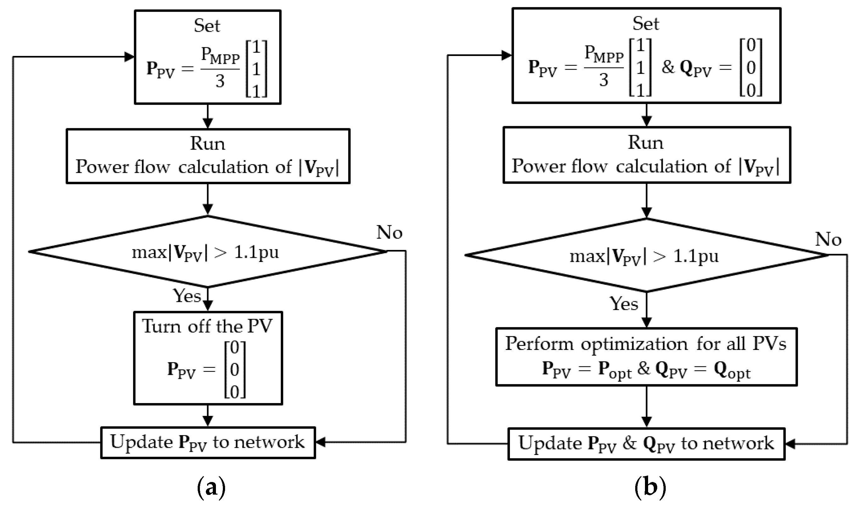
4.1. Decentralized Overvoltage Control (DOVC)

The decentralized overvoltage control receives ${\mathrm{P}}_{\mathrm{MPP}}$ data from each inverter and load data from each node and after power flow analysis simply turns off any inverter where the voltage at the bus is 10% over the rated level. The flowchart of the control is shown in Figure 5a. In this control, only active power is controlled. Initially, the available active power from the PV system is divided equally across the three phases. Then, the power flow analysis is conducted to determine the bus voltage as in Section 2. When there is an overvoltage on a PV bus, the PV power at this bus would be turned off until the voltage is under the limit, when it will be turned on.

4.2. Decentralized Power Dispatch Control (DPDC)

The flowchart of this control is shown in Figure 5b. The initial steps of the DPDC are the same as the DOVC, the active power is divided the 3-phase equally without reactive power. The controller receives ${\mathrm{P}}_{\mathrm{MPP}}$ data from each inverter and load data from each node and a power flow calculation as in Section 2 is taken to get the voltage magnitude values. As seen in the flowchart, when no overvoltage issues exist, the PV inverters output equally on the three phases, which is similar to the DOVC. In the case of overvoltage, multi-objective optimization is applied. The purpose of the optimization is to find the active and reactive powers of PV inverters to maximize the dispatched active power and minimize the reactive power absorbed while maintaining the limit of the voltage.

The power factor of the PV inverter is kept higher than $p{f}_{\min }$ or 0.9 [38] so that the relation between active and reactive power is shown as Equation (7).

$$\left|{\mathrm{Q}}_{\mathrm{PV}}\right|\le {\mathrm{P}}_{\mathrm{PV}}\sqrt{1/p{f}_{\min }^2-1}$$

(7)

The optimization uses the fmincon function on MATLAB [39]. The construction of the optimization includes the specification of the objective function, boundaries, initial points, and constraints. The objective function is shown in (8). In the system of ${\mathrm{N}}_{\mathrm{PV}}$ inverters, the total active power delivered from the PV inverters to their buses is maximized. The reactive power is negative to reduce the voltage level. Thus, there are two objectives of this control, including maximizing active power and minimizing reactive power.

$$\mathrm{Objective}\left(P_{\mathrm{PV}\left(\mathrm{i}\right)},Q_{\mathrm{PV}\left(\mathrm{i}\right)}\right)=\min \left(-{\displaystyle \sum }_{\mathrm{i}=1}^{{\mathrm{N}}_{\mathrm{PV}}}\left[111\right]P_{\mathrm{PV}\left(\mathrm{i}\right)}+{\displaystyle \sum }_{\mathrm{i}=1}^{{\mathrm{N}}_{\mathrm{PV}}}\left[111\right]Q_{\mathrm{PV}\left(\mathrm{i}\right)}\right)$$

(8)

The lower and upper bounds of active and reactive power are shown in (9) and (10), and the linear inequality conditions at PV bus $\mathrm{i}$ are shown in Equations (11) and (12).

$$\left[\begin{array}{c}0\\ 0\\ 0\end{array}\right]\le P_{\mathrm{PV}\left(\mathrm{i}\right)}\le \left[\begin{array}{c}1\\ 1\\ 1\end{array}\right]{\mathrm{P}}_{\mathrm{MPP}}$$

(9)

$$-\left[\begin{array}{c}1\\ 1\\ 1\end{array}\right]\left({\mathrm{P}}_{\mathrm{MPP}}\sqrt{1/p{f}_{\min }^2-1}\right)\le Q_{\mathrm{PV}\left(\mathrm{i}\right)}\le \left[\begin{array}{c}0\\ 0\\ 0\end{array}\right]$$

(10)

$$\left[111\right]P_{\mathrm{PV}\left(\mathrm{i}\right)}\le {\mathrm{P}}_{\mathrm{MPP}}$$

(11)

$$-Q_{\mathrm{PV}\left(\mathrm{i}\right)}\le \left[\begin{array}{ccc}\mathrm{m}& 0& 0\\ 0& \mathrm{m}& 0\\ 0& 0& \mathrm{m}\end{array}\right]P_{\mathrm{PV}\left(\mathrm{i}\right)}\mathrm{where}\mathrm{m}=\sqrt{1/p{f}_{\min }^2-1}$$

(12)

The non-linear inequality condition is shown in (13). The voltage magnitude $\left|V_{\mathrm{PV}}\right|$ in (13) is a function of $P_{\mathrm{PV}}$ and $Q_{\mathrm{PV}}$, and it is computed using the Newton–Raphson power flow as mentioned in Section 2. This step of power flow calculation for $\left|V_{\mathrm{PV}}\right|$ is also described in the second block of Figure 5b.

$$\left|V_{\mathrm{PV}\left(\mathrm{i}\right)}\right|\le \left[\begin{array}{c}1\\ 1\\ 1\end{array}\right]1.1$$

(13)

The initial or starting points of the active and reactive powers are shown in (14). The active power of each phase is equal to an amount of 50% the initial setting. In this network configuration, the initial points are chosen to satisfy all constraints, especially the voltage limit.

$$P_{\mathrm{PV}\left(\mathrm{i}\right)}^{\left(0\right)}=\left[\begin{array}{c}1\\ 1\\ 1\end{array}\right]\frac{{\mathrm{P}}_{\mathrm{MPP}}}{6}\mathrm{and}{Q}_{\mathrm{PV}\left(\mathrm{i}\right)}^{\left(0\right)}=\left[\begin{array}{c}0\\ 0\\ 0\end{array}\right]$$

(14)

The control sequence is summarized as follows. The power profiles are applied to the loads and PV inverters. There is no reactive power applied for the PV inverters and they operate at unity power factor. The power flow is carried out to calculate the network bus voltages. These bus voltages are constantly checked and when there is no overvoltage, the system keeps running with the pre-set power profiles. When any calculated voltage reaches a limit, the optimization control is applied to the PV inverters. Reactive power is consumed by the PV inverters to reduce the voltage level. When the reactive power reaches the maximum capacity set by the power factor limit, the active power from the inverters is curtailed. The active power curtailment is the last option of the control when the reactive power capacity is at maximum level or power factor is at minimum acceptable value.

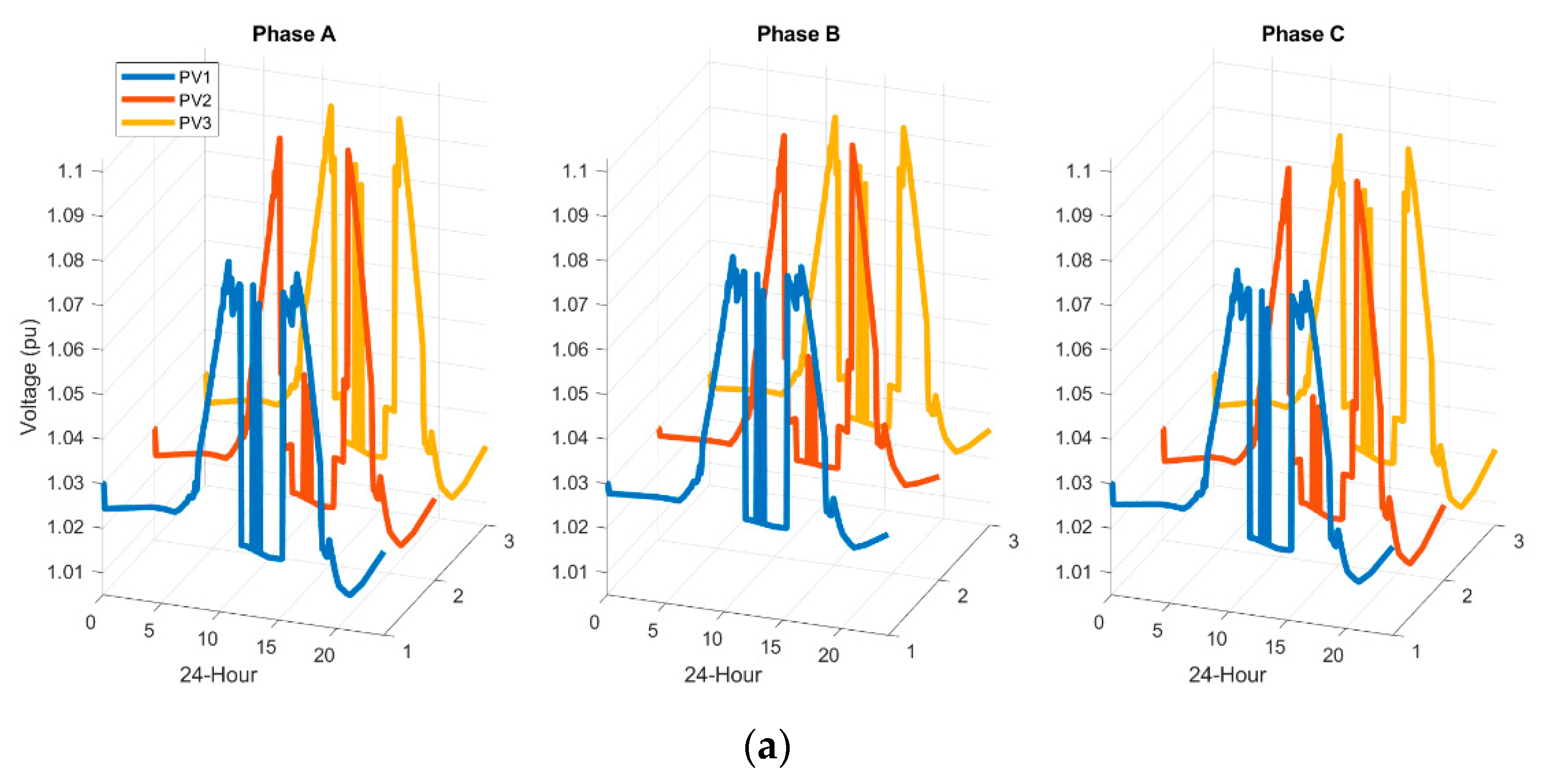
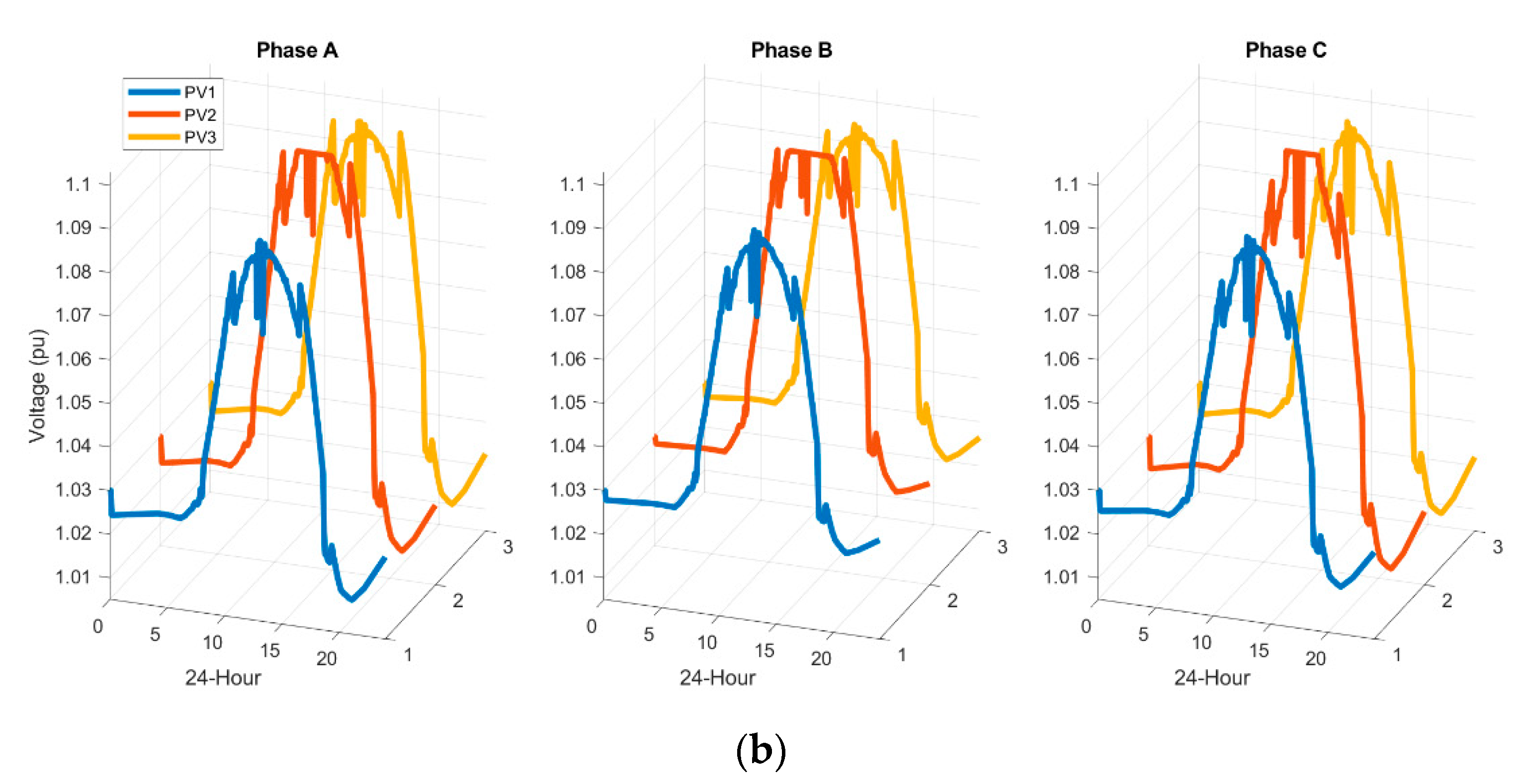
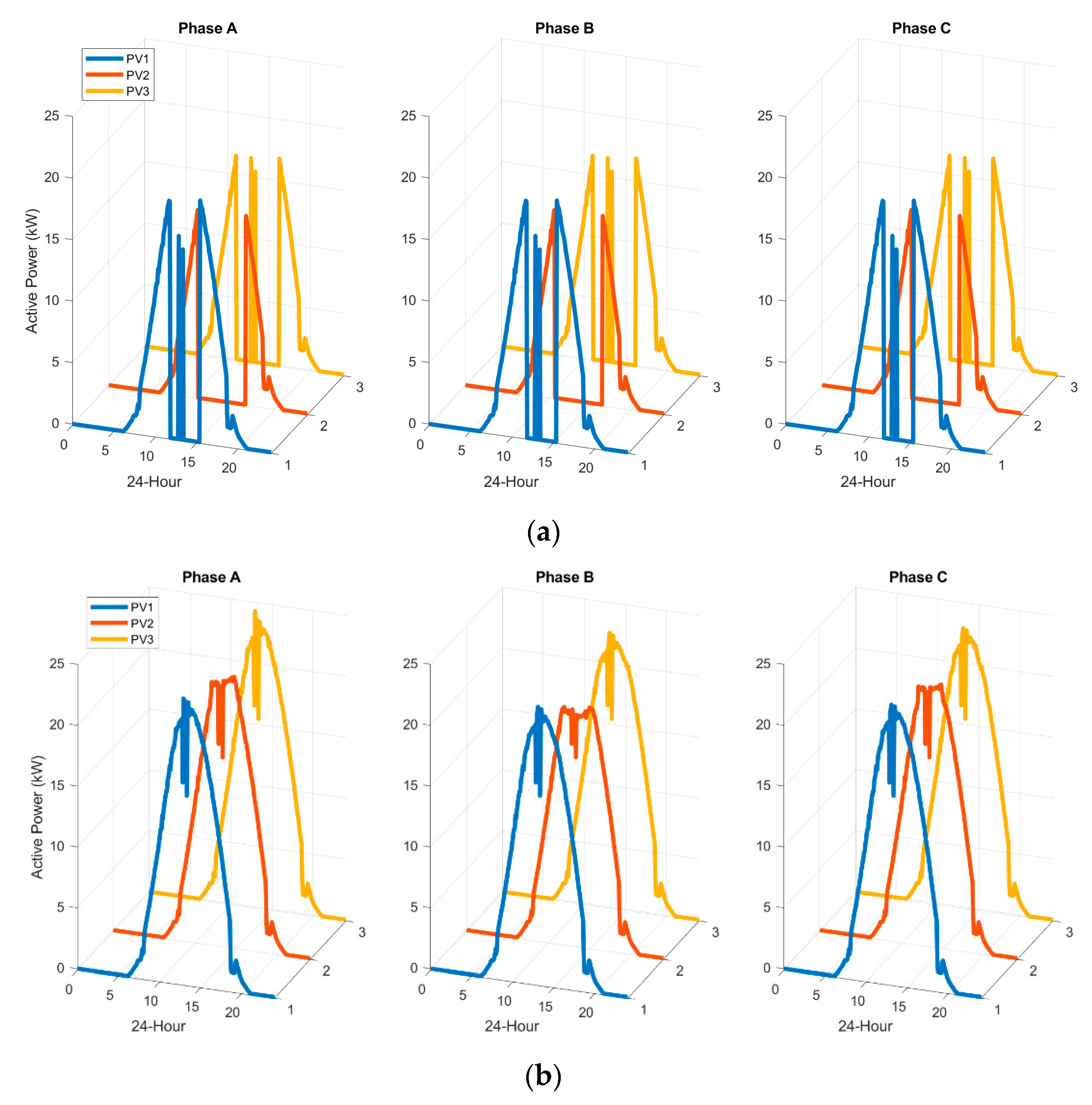
5. Simulation Results

The simulation results for the two decentralized control methods are shown in Figure 6, Figure 7 and Figure 8. The results are placed together for comparison. As seen in Figure 6, at around 11 a.m., the voltage increases to 1.1 pu and the DOVC turns the PV off and turns it on again at around 4 p.m. The DPDC performs an optimization at each time step and sets reactive and active power levels to keep the voltage at or below 1.1 pu.

In Figure 7, the DOVC strategy has PVs turned off and there is no active power delivered from 11 a.m. to 4 p.m. due to voltage constraints. For the DPDC, the algorithm initially responds to overvoltage conditions by absorbing reactive power while the active power keeps close to the ${\mathrm{P}}_{\mathrm{MPP}}$ profile. Around noon, the limit on reactive power absorption results in the curtailed active power at PV2 to maintain the voltage level under 1.1 pu.

The reactive power and power factor of DPDC are shown in Figure 8. The reactive power is negative or being absorbed by the PVs and the power factor of the PV inverters is kept above its minimum threshold of 0.9.

The maximum energy of the solar power profile over the simulated 24-h period is 1.494 MWh. The total energy delivered using the DOVC is 0.626 MWh or 41.92% of the available total. The energy generated from the DPDC is 1.484 MWh or 99.39% of the maximum available total. The use of control strategies, as outlined, could greatly increase the capacity to host PV systems within a distribution network. Combined with demand-side management and energy storage, the generation peaks resulting from high PV penetration could be prevented from disrupting DSO voltage regulation requirements while delivering maximum renewable energy benefits to end-users.

6. Discussion

The Newton–Raphson method for power flow analysis of unbalanced 3-phase systems in the format of current mismatch in polar coordinates has been presented in detail. After the construction of the power flow formulas in matrix form, they are applied to an unbalanced 3-phase benchmark network. The network operation is simulated over a full day with residential loads and PV inverters in the network. The effect of voltage rise due to reverse power flow from the PV inverters is investigated and control strategies based on ideal decentralized communication are applied for the overvoltage scenarios. Initially, reactive power support levels from each of the PV inverters to reduce the node voltages are controlled by the optimization method. The power factors of the PV inverters are considered when applying the reactive powers of the PV inverters in relation to the active power supplied. The construction of the optimization problem is also presented in the matrix form, which is consistent with the power flow formulas.

The formulas of power flow are reconstructed from the expression of a single-phase into a matrix form where each matrix consists of three phase components. This gives advantages of reducing the complexity of the formulas and this compact matrix form is constructed from the perspective of a programmer. For comparison to the conventional formulas, Equations (1) and (2) are rewritten in Equations (15) and (16). These two are put “side-by-side” with the two equations from Table 1 as seen in Equations (17) and (18) for comparison.

$$\mathsf{\Delta }{\mathrm{I}}_{\mathrm{r}\left(\mathrm{i}\right)}^{\mathrm{p}}=\frac{{\mathrm{P}}_{\mathrm{sh}\left(\mathrm{i}\right)}^{\mathrm{p}}\cos {\mathsf{\delta }}_{\mathrm{i}}^{\mathrm{p}}+{\mathrm{Q}}_{\mathrm{sh}\left(\mathrm{i}\right)}^{\mathrm{p}}\sin {\mathsf{\delta }}_{\mathrm{i}}^{\mathrm{p}}}{\left|{\mathrm{V}}_{\mathrm{i}}^{\mathrm{p}}\right|}-{{\displaystyle \sum }}_{\mathrm{k}=1}^{\mathrm{N}}{{\displaystyle \sum }}_{\mathrm{q}=\mathrm{a},\mathrm{b},\mathrm{c}}\left|{\mathrm{V}}_{\mathrm{k}}^{\mathrm{q}}\right|\left({\mathrm{G}}_{\mathrm{ik}}^{\mathrm{pq}}\cos {\mathsf{\delta }}_{\mathrm{k}}^{\mathrm{p}}-{\mathrm{B}}_{\mathrm{ik}}^{\mathrm{pq}}\sin {\mathsf{\delta }}_{\mathrm{k}}^{\mathrm{p}}\right)$$

(15)

$$\frac{\partial \mathsf{\Delta }{\mathrm{I}}_{\mathrm{r}\left(\mathrm{i}\right)}^{\mathrm{p}}}{\partial {\mathsf{\delta }}_{\mathrm{i}}^{\mathrm{p}}}=-\frac{{\mathrm{P}}_{\mathrm{sh}\left(\mathrm{i}\right)}^{\mathrm{p}}\sin {\mathsf{\delta }}_{\mathrm{i}}^{\mathrm{p}}-{\mathrm{Q}}_{\mathrm{sh}\left(\mathrm{i}\right)}^{\mathrm{p}}\cos {\mathsf{\delta }}_{\mathrm{i}}^{\mathrm{p}}}{\left|{\mathrm{V}}_{\mathrm{i}}^{\mathrm{p}}\right|}+\left|{\mathrm{V}}_{\mathrm{i}}^{\mathrm{p}}\right|\left({\mathrm{G}}_{\mathrm{ii}}^{\mathrm{pp}}\sin {\mathsf{\delta }}_{\mathrm{i}}^{\mathrm{p}}+{\mathrm{B}}_{\mathrm{ii}}^{\mathrm{pp}}\cos {\mathsf{\delta }}_{\mathrm{i}}^{\mathrm{p}}\right)$$

(16)

$$\mathsf{\Delta }{I}_{\mathrm{r}\left(\mathrm{i}\right)}=\left(P_{\mathrm{sh}\left(\mathrm{i}\right)}\odot \cos {\delta }_{\mathrm{i}}+Q_{\mathrm{sh}\left(\mathrm{i}\right)}\odot \sin {\delta }_{\mathrm{i}}\right)\oslash \left|V_{\mathrm{i}}\right|-{{\displaystyle \sum }}_{\mathrm{k}=1}^{\mathrm{N}}\left(G_{\mathrm{ik}}\mathrm{diag}\left(\cos {\delta }_{\mathrm{k}}\right)-B_{\mathrm{ik}}\mathrm{diag}\left(\sin {\delta }_{\mathrm{k}}\right)\right)\mathrm{diag}\left(\left|V_{\mathrm{k}}\right|\right){\left[111\right]}^{\mathrm{T}}$$

(17)

$$\frac{\partial \mathsf{\Delta }{I}_{\mathrm{r}\left(\mathrm{i}\right)}}{\partial {\delta }_{\mathrm{i}}}=-{\left(\left(\left(P_{\mathrm{sh}\left(\mathrm{i}\right)}\odot \sin {\delta }_{\mathrm{i}}-Q_{\mathrm{sh}\left(\mathrm{i}\right)}\odot \cos {\delta }_{\mathrm{i}}\right)\oslash \left|V_{\mathrm{i}}\right|\right)\left[111\right]\right)}^{\mathrm{T}}+\left(G_{\mathrm{ii}}\mathrm{diag}\left(\sin {\delta }_{\mathrm{i}}\right)+B_{\mathrm{ii}}\mathrm{diag}\left(\cos {\delta }_{\mathrm{i}}\right)\right)\mathrm{diag}\left(\left|V_{\mathrm{i}}\right|\right)$$

(18)

In Equations (17) and (18), the phase index ($\mathrm{p}=\mathrm{a},\mathrm{b},\mathrm{c}$) is omitted. This means that Equation (17) presents the current mismatch $\mathsf{\Delta }{I}_{\mathrm{r}}$ for 3-phase components while in Equation (15), the current $\mathsf{\Delta }{\mathrm{I}}_{\mathrm{r}}^{\mathrm{p}}$ presents only a single phase. Furthermore, in Equation (15), there are two sum loops for the $\mathrm{k}$ ($\mathrm{k}=1\mathrm{to}\mathrm{k}=\mathrm{N}$) and $\mathrm{q}$ ($\mathrm{q}=\mathrm{a},\mathrm{b},\mathrm{c}$), while there is only one sum loop in Equation (17). The matrix expression, therefore, reduces the program loops and reduces the code verification burden. The Hadamard or element-wise operations $\odot$, $\oslash$, °² and diag() are practical in coding.

The matrix presentation is also used in other papers of power flow calculation but there are no complete formulas in the specific Newton–Raphson of the current mismatch in polar coordinates. Moreover, the consistency of using the matrix form for both the power flow and optimization construction is mentioned. There are several papers on power flow analysis methods and these methods are verified by static power flow results [6,7,8,9,10,11,12,13,14,15,16,17,18,19,20,21,22,23,24]. Other research shows optimization controls, over a time period, applied to the network but the power flow calculations are briefly introduced or neglected [29,30,31,32,33]. This paper presents a complete power flow calculation in matrix form, from the construction of the admittance matrix illustrated in an unbalanced benchmark network over a full day and the optimization control strategy in matrix form and effects of the solar PV inverters in the network.

In this paper, the decentralized approach is applied, which ignores practical issues of communication and device delay. It is the first step to further investigation of other control methods and scenarios including battery storage, demand-side management, the effect of communication errors, lack of bus information and fault analysis. The power flow formulas are applied for the constant power P-Q buses with a slack bus. From this base formulation, it is possible to expand the matrix expression for a constant power-voltage P-V bus, transformer with tap change, FACTS and other load types, such as constant impedance Z, constant current I and combined impedance–current–power ZIP with both wye and delta connections. The formula may also be presented in an integrated matrix and complex form. This research is an environment for further investigation of high penetration PV energy into the distribution network and future smart microgrids and optimization of renewable energy management in a stable grid with dynamic changes of residential loads and weather conditions.

7. Conclusions

The research has presented a detailed formulation and process to perform power flow analysis in an unbalanced 3-phase distribution network using the Newton–Raphson method in the format of current mismatch in polar coordinates. The network is described in a matrix format suited to the development of a programmed solution. A benchmark 20-node network with unbalanced distribution lines, PV inverters, and loads was built using MATLAB/Simulink to verify the matrix model. Power flow analysis on this network for a sunny day showed that node voltages without control could rise to 1.3 pu.

To address this overvoltage issue, two decentralized control methods, using a power flow analysis with the matrix model, were applied to the network. A decentralized overvoltage controller (DOVC) simply turns off any inverter where the voltage at the bus is 10% over the rated level. A decentralized power dispatch controller (DPDC) performs a multi-objective optimization to find the active and reactive powers of PV inverters to maximize the dispatched active power and minimize the reactive power absorbed while maintaining the voltage and power factor within limits. The detailed construction of the optimization problem for the 3-phase network in matrix form which is consistent with the power flow calculation is also described. Simulation with the control methods over a day shows that the total active power of the on/off and optimized controllers deliver 41.92% and 99.39% of the available solar power, respectively, while maintaining the network node voltages within limits.

References

1. Shayani, R.A.; de Oliveira, M.A.G. Photovoltaic Generation Penetration Limits in Radial Distribution Systems. IEEE Trans. Power Syst. 2011, 26, 1625–1631. [Google Scholar] [CrossRef]
2. Budka, K.; Deshpande, J.; Thottan, M. Communication Networks for Smart Grids: Making Smart Grid Real; Computer Communications and Networks; Springer: Berlin, Germany, 2014; ISBN 978-1-4471-6302-2. [Google Scholar]
3. Thomas, M.; McDonald, J. Power System SCADA and Smart Grids; Taylor & Francis: Abingdon, UK, 2015. [Google Scholar]
4. Saadat, H. Power System Analysis; WCB/McGraw Hill: New York, NY, USA, 1999; ISBN 0-07-561634-3. [Google Scholar]
5. Glover, J.D.; Sarma, M.S.; Overbye, T.J. Power System Analysis and Design; Cengage Learning: Boston, MA, USA, 2017; ISBN 978-1-305-63213-4. [Google Scholar]
6. Sereeter, B.; Vuik, C.; Witteveen, C. On a Comparison of Newton-Raphson Solvers for Power Flow Problems; Report 17-7; Delft Institute of Applied Mathematics, Delft University of Technology: Delft, The Netherlands, 2017. [Google Scholar]
7. Sereeter, B.; Vuik, K.; Witteveen, C. Newton Power Flow Methods for Unbalanced Three-Phase Distribution Networks. Energies 2017, 10, 1658. [Google Scholar] [CrossRef]
8. Rajaei, N.; Ahmed, M.H.; Salama, M.M.A. A novel Newton-Raphson algorithm for power flow analysis in the presence of constant current sources. In Proceedings of the 2016 IEEE/PES Transmission and Distribution Conference and Exposition (T&D), Dallas, TX, USA, 3–5 May 2016; pp. 1–5. [Google Scholar] [CrossRef]
9. Zhang, X.P.; Ju, P.; Handschin, E. Continuation three-phase power flow: A tool for voltage stability analysis of unbalanced three-phase power systems. IEEE Trans. Power Syst. 2005, 20, 1320–1329. [Google Scholar] [CrossRef]
10. Chindris, M.; Sudria i Anderu, A.; Bud, C.; Tomoiaga, B. The load flow calculation in unbalanced radial electric networks with distributed generation. In Proceedings of the 2007 9th International Conference on Electrical Power Quality and Utilisation, Barcelona, Spain, 9–11 October 2007; pp. 1–5. [Google Scholar] [CrossRef]
11. Aguirre, R.A.; Bobis, D.X.S. Improved power flow program for unbalanced radial distribution systems including voltage dependent loads. In Proceedings of the 2016 IEEE 6th International Conference on Power Systems (ICPS), New Delhi, India, 4–6 March 2016; pp. 1–6. [Google Scholar] [CrossRef]
12. AlHajri, M.F.; El-Hawary, M.E. Exploiting the Radial Distribution Structure in Developing a Fast and Flexible Radial Power Flow for Unbalanced Three-Phase Networks. IEEE Trans. Power Deliv. 2010, 25, 378–389. [Google Scholar] [CrossRef]
13. Garces, A. A Linear Three-Phase Load Flow for Power Distribution Systems. IEEE Trans. Power Syst. 2016, 31, 827–828. [Google Scholar] [CrossRef]
14. Li, H.; Yan, X.; Yan, J.; Zhang, A.; Zhang, F. A Three-Phase Unbalanced Linear Power Flow Solution with PV Bus and ZIP Load. IEEE Access 2019, 7, 138879–138889. [Google Scholar] [CrossRef]
15. Wang, Y.; Zhang, N.; Li, H.; Yang, J.; Kang, C. Linear three-phase power flow for unbalanced active distribution networks with PV nodes. CSEE J. Power Energy Syst. 2017, 3, 321–324. [Google Scholar] [CrossRef]
16. Chatterjee, S.; Mandal, S. A novel comparison of Gauss-Seidel and Newton-Raphson methods for load flow analysis. In Proceedings of the 2017 International Conference on Power and Embedded Drive Control (ICPEDC), Chennai, India, 16–18 March 2017; pp. 1–7. [Google Scholar] [CrossRef]
17. Muzzammel, R.; Ahsan, M.; Ahmad, W. Non-linear analytic approaches of power flow analysis and voltage profile improvement. In Proceedings of the 2015 Power Generation System and Renewable Energy Technologies (PGSRET), Islamabad, Pakistan, 10–11 June 2015; pp. 1–7. [Google Scholar] [CrossRef]
18. Kamel, S.; Abdel-Akher, M.; El-Nemr, M. Hybrid power and current mismatches Newton-Raphson load-flow analysis for solving power systems with voltage controlled devices. In Proceedings of the 14th International Middle East Power Systems Conference (MEPCON), Cairo, Egypt, 19–21 December 2010; pp. 763–768. [Google Scholar]
19. Sairam, S. Analysis of ZIP Load Modeling in Power Transmission System. Int. J. Control Autom. 2018, 11, 11–24. [Google Scholar] [CrossRef]
20. Okyere, H.K.; Nouri, H.; Moradi, H.; Li, Z. Statcom and load tap changing transformer (LTC) in Newton Raphson Power Flow: Bus voltage constraint and losses. In Proceedings of the 42nd International Universities Power Engineering Conference, Brighton, UK, 4–6 September 2007; pp. 1013–1018. [Google Scholar] [CrossRef]
21. Santos, N.M.; Dias, O.; Pires, V.F. Use of an Interline Power Flow Controller Model for Power Flow Analysis. Energy Procedia 2012, 14, 2096–2101. [Google Scholar] [CrossRef] [Green Version]
22. Kamel, S.; Jurado, F.; Chen, Z.; Abdel-Akher, M.; Ebeed, M. Developed generalised unified power flow controller model in the Newton–Raphson power-flow analysis using combined mismatches method. Iet Gener. Transm. Distrib. 2016, 10, 2177–2184. [Google Scholar] [CrossRef]
23. Ren, B.X.; Cai, H.; Du, W.J.; Wang, H.F.; Fan, L.L. Analysis of power flow control capability of a unified power flow controller to be installed in a real Chinese power network. In Proceedings of the 12th IET International Conference on AC and DC Power Transmission (ACDC 2016), Beijing, China, 28–29 May 2016; pp. 1–6. [Google Scholar] [CrossRef]
24. Yang, J.; Xu, Z.; Wang, W.; Cai, H. Implementation of a novel unified power flow controller into Newton-Raphson load flow. In Proceedings of the 2017 IEEE Power Energy Society General Meeting, Chicago, IL, USA, 16–20 July 2017; pp. 1–5. [Google Scholar] [CrossRef]
25. Schneider, K.P.; Mather, B.A.; Pal, B.C.; Ten, C.-W.; Shirek, G.J.; Zhu, H.; Fuller, J.C.; Pereira, J.L.R.; Ochoa, L.F.; de Araujo, L.R.; et al. Analytic Considerations and Design Basis for the IEEE Distribution Test Feeders. IEEE Trans. Power Syst. 2018, 33, 3181–3188. [Google Scholar] [CrossRef]
26. IEEE PES AMPS DSAS Test Feeder. Available online: https://site.ieee.org/pes-testfeeders/resources/ (accessed on 6 March 2020).
27. Strunz, K.; Abbasi, E.; Fletcher, R.; Hatziargyriou, N.; Iravani, R.; Joos, G. TF C6.04.02: TB 575—Benchmark Systems for Network Integration of Renewable and Distributed Energy Resources; CIGRE: Paris, France, 2014; pp. 54–62. ISBN 978-285-873-270-8. [Google Scholar]
28. Clua, J.; Sainz, L.; Corcoles, F. Three-phase transformer modeling for unbalanced harmonic power flow studies. In Proceedings of the Ninth International Conference on Harmonics and Quality of Power, Orlando, FL, USA, 1–4 October 2000; Cat. No.00EX441. Volume 2, pp. 726–731. [Google Scholar] [CrossRef]
29. Guggilam, S.S.; Dall’Anese, E.; Chen, Y.C.; Dhople, S.V.; Giannakis, G.B. Scalable Optimization Methods for Distribution Networks With High PV Integration. IEEE Trans. Smart Grid 2016, 7, 2061–2070. [Google Scholar] [CrossRef]
30. Craciun, B.; Sera, D.; Man, E.A.; Kerekes, T.; Muresan, V.A.; Teodorescu, R. Improved voltage regulation strategies by PV inverters in LV rural networks. In Proceedings of the 2012 3rd IEEE International Symposium on Power Electronics for Distributed Generation Systems (PEDG), Aalborg, Denmark, 25–28 June 2012; pp. 775–781. [Google Scholar] [CrossRef]
31. Levis, C. Smart Inverters for Distributed PV Network Management. Ph.D. Thesis, Cork Institute of Technology, Cork, Ireland, 2019. [Google Scholar]
32. Samadi, A.; Shayesteh, E.; Eriksson, R.; Rawn, B.; Soder, L. Multi-objective coordinated droop-based voltage regulation in distribution grids with PV systems. Renew. Energy 2014, 71, 315–323. [Google Scholar] [CrossRef]
33. Hou, J.; Xu, Y.; Liu, J.; Xin, L.; Wei, W. A multi-objective volt-var control strategy for distribution networks with high PV penetration. In Proceedings of the 10th International Conference on Advances in Power System Control, Operation Management (APSCOM 2015), Hong Kong, China, 8–12 November 2015; pp. 1–6. [Google Scholar] [CrossRef]
34. Zhang, Y.; Lu, Y. A novel newton current equation method on power flow analysis in microgrid. In Proceedings of the 2009 IEEE Power Energy Society General Meeting, Calgary, AB, Canada, 26–30 July 2009; pp. 1–6. [Google Scholar] [CrossRef]
35. Le Nguyen, H. Newton-Raphson method in complex form. IEEE Trans. Power Syst. 1997, 12, 1355–1359. [Google Scholar] [CrossRef]
36. MATLAB Generalized Mutual Inductance. Available online: https://www.mathworks.com/help/physmod/sps/powersys/ref/mutualinductance.html#f3-2480259 (accessed on 6 March 2020).
37. Markiewicz, H.; Klajn, A. Voltage Disturbances Standard EN 50160—Voltage Characteristics in Public Distribution Systems; Wroclaw University of Technology: Wroclaw, Poland, 2004. [Google Scholar]
38. NRS 097-2-3. Grid Interconnection of Embedded Generation, Part 2: Small-Scale Embedded Generation, Section 3: Simplified Utility Connection Criteria for Low-Voltage Connected Generators; Standard, South African National Standards (SANS): Midrand, South Africa, 2014. [Google Scholar]
39. MATLAB Fmincon. Available online: https://www.mathworks.com/help/optim/ug/fmincon.html (accessed on 6 March 2020).
Figure 1. Unbalanced 3-phase power flow calculation steps.
Energies 13 03011 g001
Figure 2. MATLAB/Simulink network.
Energies 13 03011 g002
Figure 3. Daily power profiles (a) P MPP per each PV inverter (b) P Load and Q Load per each phase.
Energies 13 03011 g003
Figure 4. Voltage at PV buses without control.
Energies 13 03011 g004
Figure 5. Control flowcharts: (a) decentralized overvoltage control (DOVC), (b) decentralized power dispatch control (DPDC).
Energies 13 03011 g005
Figure 6. Voltage at PV buses: (a) DOVC, (b) DPDC.
Energies 13 03011 g006aEnergies 13 03011 g006b
Figure 7. Active Power at PV buses: (a) OVC, (b) DPDC.
Energies 13 03011 g007
Figure 8. DPDC results: (a) reactive power, (b) power factor.
Energies 13 03011 g008