On-Line Estimation of the Ultrasonic Power in a Continuous Flow Sonochemical Reactor

Abstract

Sonochemical reactors can be very effective in many applications, including: degradation of chemical pollutants, inactivation of microorganisms, or production of biofuels. However, due to various factors, the ultrasonic power that is dissipated into sonicated liquid may vary in time. Hence, it is obvious that the ultrasonic power must be known for an optimal design and operation of the sonoreactor. In this paper, we present a method for on-line estimation of the ultrasonic power in continuous flow sonoreactors. In this method, we design an observer that estimates unknown model parameters by using a mathematical model of the sonoreactor and by measuring input and output temperatures in the sonoreactor system. The effectiveness of the method is shown for a simulated and real continuous flow sonoreactors. We also discuss the possibilities of ultrasonic power stabilization by using control algorithms.

1. Introduction

The use of ultrasonic waves to improve the efficiency of chemical reactions is the subject of intensive research and the number of applications for ultrasonic devices is growing rapidly. Techniques related to sonochemistry and the phenomenon of cavitation are the basis for obtaining many natural products (e.g., proteins, oils, dyes, spices, bioethanol, etc.) without using toxic reagents, shortening the reaction time, increasing the reaction efficiency, product purity, improving efficiency of production processes, and reduction of reagent consumption [1,2,3,4,5]. The ultrasounds can also be used in degradation of chemical pollutants in water [6]; thus, the sonochemistry is seen as a "green" future technology, beneficial to the environment [1]. It is also well-known that ultrasounds are responsible for the cavitation phenomenon which is the formation, growth, and collapse of bubbles in the liquid medium. The result of the ultrasonic cavitation is the production of free radicals (e.g., hydroxyl radicals) that are very effective in the inactivation of microorganisms [7]. In turn, the results presented in a study [8] show that airborne viruses such as severe acute respiratory syndrome (SARS) coronavirus or influenza viruses can also be inactivated by generating ultrasonic vibrations.

Recent papers show a growing interest in continuous flow sonochemical reactors, since they are often more efficient and more flexible than batch sonoreactors [6,9,10,11,12]. However, the potential for using sonochemical reactors is still limited by a lack of knowledge about their design, operation, and performance characteristics. Experimental results show that the ultrasonic power released in the sonoreactor can be dependent on the height of the sonicated medium, temperature, pressure, or ultrasound frequency [13,14]. This means that the ultrasonic power transferred to the medium in the reactor is not constant and may vary during the normal operation of a sonoreactor. If one conducts experiments to study, for instance, the effects of the sonication power on the process performance, then it is obvious that the sonication power must be known and kept constant. The sonication power must also be known for an optimal design of a sonoreactor [12,15,16]. To determine the amount of ultrasonic power that is dissipated into a liquid medium, calorimetric methods are widely used [17,18,19]. Then, by measuring temperature changes in the sonicated liquid, it is possible to estimate the ultrasonic power. However, these methods are applied off-line, prior to the normal operation of a sonoreactor. Moreover, mathematical models used in determination of the ultrasonic power are based on many simplifying assumptions (e.g., the heat transfer between the sonoreactor and the surroundings is often neglected). Since the ultrasonic power can be affected by various factors (e.g., temperature) and may vary in time, a method for its on-line estimation is desired.

Knowing that observer-based methods for state and parameter estimation can be very effective for chemical and biochemical reactors [20,21], in the presented paper, we propose a method that is dedicated to continuous flow sonochemical reactors for on-line estimation of the ultrasonic power. Given a mathematical model of the sonoreactor and by measuring input and output temperatures in the sonoreactor system, we design an observer that estimates unknown model parameters. First, we derive a mathematical model of the sonoreactor, then the effectiveness of the presented method is shown for a simulated and real continuous flow sonoreactor. Once the ultrasonic power is known, we discuss the possibilities of its stabilization by using a controller.

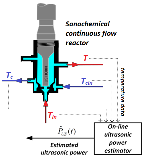
2. Materials and Methods

The complete measuring setup is shown in Figure 1. The main element of the measuring setup is the continuous flow sonoreactor (REACTOR) with a cooling jacket (CJ) adapted to work with the Branson 450 sonifier (maximal input electric power 350 W, ultrasonic frequency 20 kHz). The ultrasonic power is pulsed (frequency: 1 Hz) and can be controlled manually by changing its duty cycle. The ultrasonic horn with diameter ½″ (US HORN) is attached to the reactor via a screw connection. The jacketed sonoreactor has three connections to the reaction vessel (volume about 36 mL) and two connections to the cooling jacket (volume about 5 mL). The topmost connection of the reaction vessel is used to vent the reactor and the other connections are used as input and output for reagents. The sonoreactor has two circuits: the cooling circuit through the cooling jacket with the input “CJ IN” and the output “CJ OUT”, and the main circuit through the reaction vessel (REACTOR) with the input “REACTOR IN” and the output “REACTOR OUT” (Figure 1). All the temperature values, including input and output temperatures in each circuit and ambient temperature, are measured by using PT100 sensors connected to the multi-channel temperature data logger (APAR, model AR207; sampling period: 1 s). The flow rates in both circuits are controlled by using peristaltic pumps (Masterflex, model no. 77521-57) and the programmable logic controller (Allen Bradley, Compact Logix).

Both reactor circuits are fed with a cold water from a water bath with the immersion cooler “Chiller 1” (Huber, TC40E). For a better stabilization of the inlet temperatures, the additional chiller “Chiller 2” (Hailea, HC-130A) is included in the cooling jacket circuit (Figure 1). The medium exiting the reactor vessel can be redirected through valve V2 back to the water bath or to the conductivity meter “CDM” (Elmetron, Model CC-401), operating in the on-line mode. By measuring the conductivity, it is possible to study the mixing flow patterns in the reactor vessel.

3. Results

3.1. Modeling of Sonochemical Reactor

Since the volume V_c of the reactor jacket is several times smaller than the vessel volume V, and the flow rates F_c of cooling water in the jacket are several times greater than the flow rates F through the vessel, it is assumed that the reactor jacket is well-mixed, and the mixing flow pattern was only analyzed in the main reactor vessel. To study the mixing pattern in the sonochemical reactor, a series of tracer pulse experiments have been performed. First, a finite amount of sodium chloride (NaCl) was injected in the input of the vessel (Figure 1). Then, by measuring the conductivity in its input and output, it was possible to determine a residence time distribution (RTD) in the vessel for different flow rates F through the reactor. If the C(t) is the output concentration of the tracer, then the RTD can be determined from the distribution of exit times curves E(t) [22,23]:

$$E(t)=\frac{C(t)}{{\displaystyle \underset{0}{\overset{\infty }{\int }}C(t)dt}}.$$

(1)

To show the differences between the mixing patterns, the experiments were performed when the ultrasounds are switched on or off. Figure 2 shows exit times curves E(t) for different flow rates through the reactor vessel.

The experimentally determined E(t) curves clearly show that the measured responses are delayed in time and the delay time is strictly dependent on the flow rate F. Then, one can observe a high rise of the tracer concentration (conductivity), followed by its exponential decay with a rate that is also dependent on the flow rate F. Hence, the mixing pattern in the reactor vessel can be approximated by using the first order system with a delay [22,23]:

$$\tau \frac{dC(t)}{dt}+C(t)=C_{in}(t-{\tau }_0),$$

(2)

where: C(t), C_in(t) are output and input tracer concentrations (conductivity), τ is the overall time constant, τ = V/F, and τ₀ is the delay time.

Model (2) is fitted to the experimental data by determining τ and τ₀ parameters and by using the least squares method. The black lines in Figure 2 represent model responses and

Table 1. Results of tracer pulse experiments for sonication on/off.

Sonication Off				Sonication On
F, mL/min	V, mL	τ, s	τ0, s	F, mL/min	V, mL	τ, s	τ0, s
47	54	69	44	47	35	45	6.3
76	113	89	25	62	37	36	5.2
91	47	31	23	91	39	26	4.3
138	53	23	10	138	39	17	2.3

shows model parameter values when the ultrasounds are switched on or off.

The volumes V in Table 1 are the vessel volumes determined from the definition of the overall time constant τ = V/F for the ideally mixed reactor. As it can be clearly seen, if the ultrasounds are switched on, then the differences between the calculated volume V (Table 1) and the vessel volume determined experimentally (about 36 mL) are relatively small. There are also shorter exit times in the presence of ultrasounds and we can assume that the reactor vessel is almost ideally mixed. The fact that the sonification can improve the mixing is also mentioned in other studies (e.g., [11,24,25]).

Hence, when deriving a mathematical model for the sonochemical reactor, one can assume that the reactor vessel is well-mixed. The other model assumptions are as follows: the volumes of water in the reactor vessel and jacket are constant, the heat is transferred between the reactor vessel and its jacket and between the vessel and the surroundings, and the cooling water in the reactor jacket is also well-mixed. The tracer pulse experiments have shown that the delay time in Equation (2) is about nine times smaller than the overall time constant, thus it can be neglected. Then, from mass and energy balances we have:

$$\frac{dT}{dt}=\frac{F}{V}(T_{in}-T)-\frac{UA}{\rho c_{p}V}(T-T_c)-\frac{U{A}_{amb}}{\rho c_{p}V}(T-T_{amb})+\frac{c{P}_{US}}{\rho c_{p}V},$$

(3)

$$\frac{d{T}_c}{dt}=\frac{F_c}{V_c}(T_{cin}-T_c)+\frac{UA}{\rho c_p{V}_c}(T-T_c),$$

(4)

where: F, F_c—flow rates through the vessel and jacket, respectively; V, V_c—volumes in the vessel and jacket, respectively; T_in, T_cin, T, T_c—input and output temperatures for the vessel and jacket, respectively; T_amb—ambient temperature; UA, UA_amb—the overall heat transfer coefficients between the reactor vessel and the jacket, and between the vessel and the surroundings, respectively; ρ, c_p—density and specific heat of the fluid in the vessel and jacket, respectively; P_US—maximum ultrasonic power; c—duty cycle.

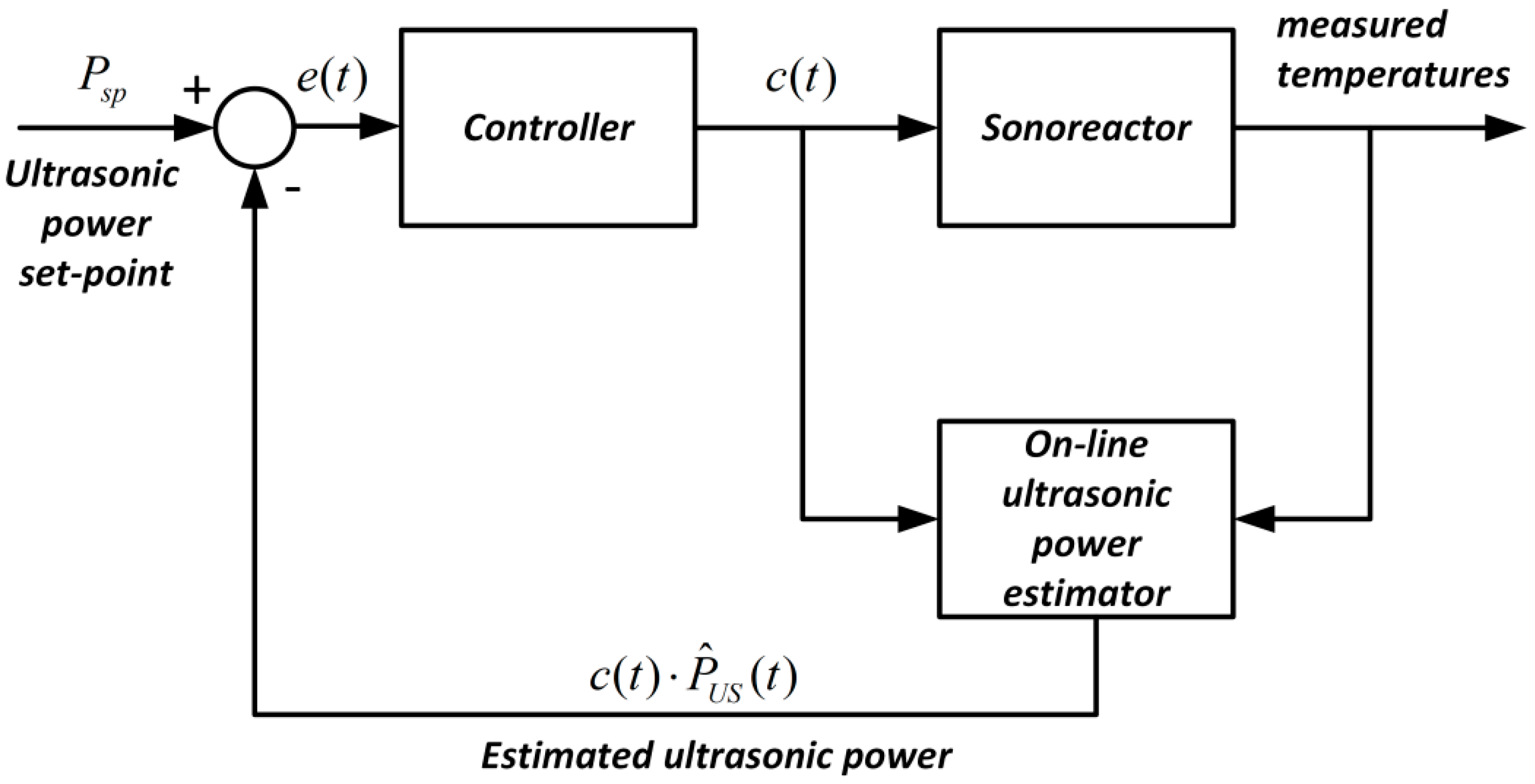
3.2. Estimation of the Ultrasonic Power

Now, by using Equations (3) and (4) it is possible to estimate on-line the unknown model parameters, i.e., the maximum ultrasonic power P_US and heat transfer coefficients UA_amb and UA. All the temperatures are measured on-line and the other model parameters in Equations (3) and (4) are known. To design an observer for on-line estimation of the unknown parameters, we follow the design procedure given in [26,27]. Model Equations (3) and (4) can be presented in a more compact form:

$$\begin{gathered} \dot{x}=Ax+Bu+E\theta , \\ {x}^T=\left[\begin{array}{cc}T& T_c\end{array}\right], u^T=\left[\begin{array}{cccc}c& T_{in}& T_{cin}& T_{amb}\end{array}\right], {\theta }^T=\left[\begin{array}{ccc}{P}_{US}& U{A}_{amb}& UA\end{array}\right], \\ A=\left[\begin{array}{cc}-\frac{F}{V}& 0\\ 0& -\frac{F_c}{V_c}\end{array}\right], B=\left[\begin{array}{cccc}0& \frac{F}{V}& 0& 0\\ 0& 0& \frac{F_c}{V_c}& 0\end{array}\right], E=\left[\begin{array}{ccc}\frac{c}{\rho c_{p}V}& -\frac{T-T_{amb}}{\rho c_{p}V}& -\frac{T-T_c}{\rho c_{p}V}\\ 0& 0& \frac{T-T_c}{\rho c_p{V}_c}\end{array}\right], \end{gathered}$$

(5)

where: x—vector of known state variables; u—vector of known inputs; θ—vector of unknown parameters; A, B, E—matrices of known model parameters and variables.

Then, the observer equations for model (5) are as follows [26]:

$$\dot{\hat{x}}=Ax+Bu+E\widehat{\theta }+A_F(\hat{x}-x),$$

(6)

$$\dot{\widehat{\theta }}=-E^T\mathsf{\Lambda }P(\hat{x}-x)$$

(7)

where: A_F—a Hurwitz matrix; P—a positive definite matrix; Λ—a diagonal matrix with positive entries; $\widehat{\theta }$—estimate of the vector of unknown parameters; $\hat{x}$—estimate of the state variables.

For model (5) and observer Equations (6) and (7), it can be shown that the state and parameter errors: $e_x=\hat{x}-x$, $e_{\theta }=\widehat{\theta }-\theta$ tend to zero as time tends to infinity. Assuming that the vector of unknown parameters θ is constant and by using Equations (5)–(7), the time derivatives of state and parameter errors are:

$${\dot{e}}_x=\dot{\hat{x}}-\dot{x}=E(\widehat{\theta }-\theta )+A_F(\hat{x}-x)=E{e}_{\theta }+A_F{e}_x,$$

(8)

$${\dot{e}}_{\theta }=\dot{\widehat{\theta }}=-\mathsf{\Lambda }{E}^{T}P{e}_x.$$

(9)

It is obvious that the only equilibrium point for the system (8) and (9) is $(e_{\theta },e_x)=(0,0)$ and to prove asymptotic stability at the origin, the following candidate Lyapunov function is used:

$$V=e_x^{T}P{e}_x+e_{\theta }^T{\mathsf{\Lambda }}^{-1}{e}_{\theta }.$$

(10)

By calculating the time derivative of (10), we have:

$$\dot{V}=e_x^{T}P{\dot{e}}_x+{\dot{e}}_x^{T}P{e}_x+2e_{\theta }^T{\mathsf{\Lambda }}^{-1}{\dot{e}}_{\theta },$$

(11)

and by substituting (8) and (9) into (11) yields:

$$\dot{V}=e_x^T(P{A}_F+A_F^{T}P)e_x+2e_x^{T}PE{e}_{\theta }-2e_{\theta }^T{E}^{T}P{e}_x=e_x^T(P{A}_F+A_F^{T}P)e_x.$$

(12)

If Q is a given positive definite and symmetric matrix and A_F is a Hurwitz matrix, then there exists a positive definite and symmetric matrix P that can be found by solving the Lyapunov equation:

$$P{A}_F+A_F^{T}P=-Q.$$

(13)

Then, from (12) and (13), it is obvious that:

$$\dot{V}=-e_x^{T}Q{e}_x\le 0,$$

(14)

and the state and parameter errors: $e_x=\hat{x}-x$, $e_{\theta }=\widehat{\theta }-\theta$ tend to zero as time tends to infinity.

The estimation of the vector of unknown parameters θ can be performed on-line by numerical integration of Equations (6) and (7) at each sampling time instant t_n = nT_s, where T_s is the sampling time. If the sampling time T_s is sufficiently small (to ensure numerical stability), then for given initial values of $\hat{x}(0)$ and $\widehat{\theta }(0)$, Equations (6) and (7) can be solved by using the explicit Euler’s method. For example, let P_US = 80 W, UA = 200 J/min/K, and UA_amb = 10 J/min/K be true parameter values for system (3) and (4). Then, from (13) for Q = 20KI₂ and A_F = –10I₂, one gets P = KI₂, where I₂ is 2 × 2 identity matrix and K > 0 is the observer gain. Figure 3 shows time courses of estimates ${\hat{P}}_{US}(t)$, $U{\hat{A}}_{amb}(t)$, and $U\hat{A}(t)$ for numerically simulated system (3) and (4) with Λ = diag(200,1,0.1) and K = 500. The ultrasonic power c(t)P_US is switched on and off between 0 and 80 W with a period T_p = 10 min.

Irrespective of the initial conditions $\hat{x}(0)$ and $\hat{\theta }(0)$, the estimates converge to true values of model parameters. It should also be noticed that in the case of proposed observer, the convergence of estimation error to zero is ensured, if the persistent excitation condition is satisfied [27]. This can be achieved, if the input signal (e.g., the ultrasonic power c(t)P_US) is manipulated in such a way that enough information on the dynamical behavior of the identified system can be gathered. In practice, a square wave input signal of an appropriate frequency can be chosen, which means that the ultrasounds are switched on and off (Figure 3).

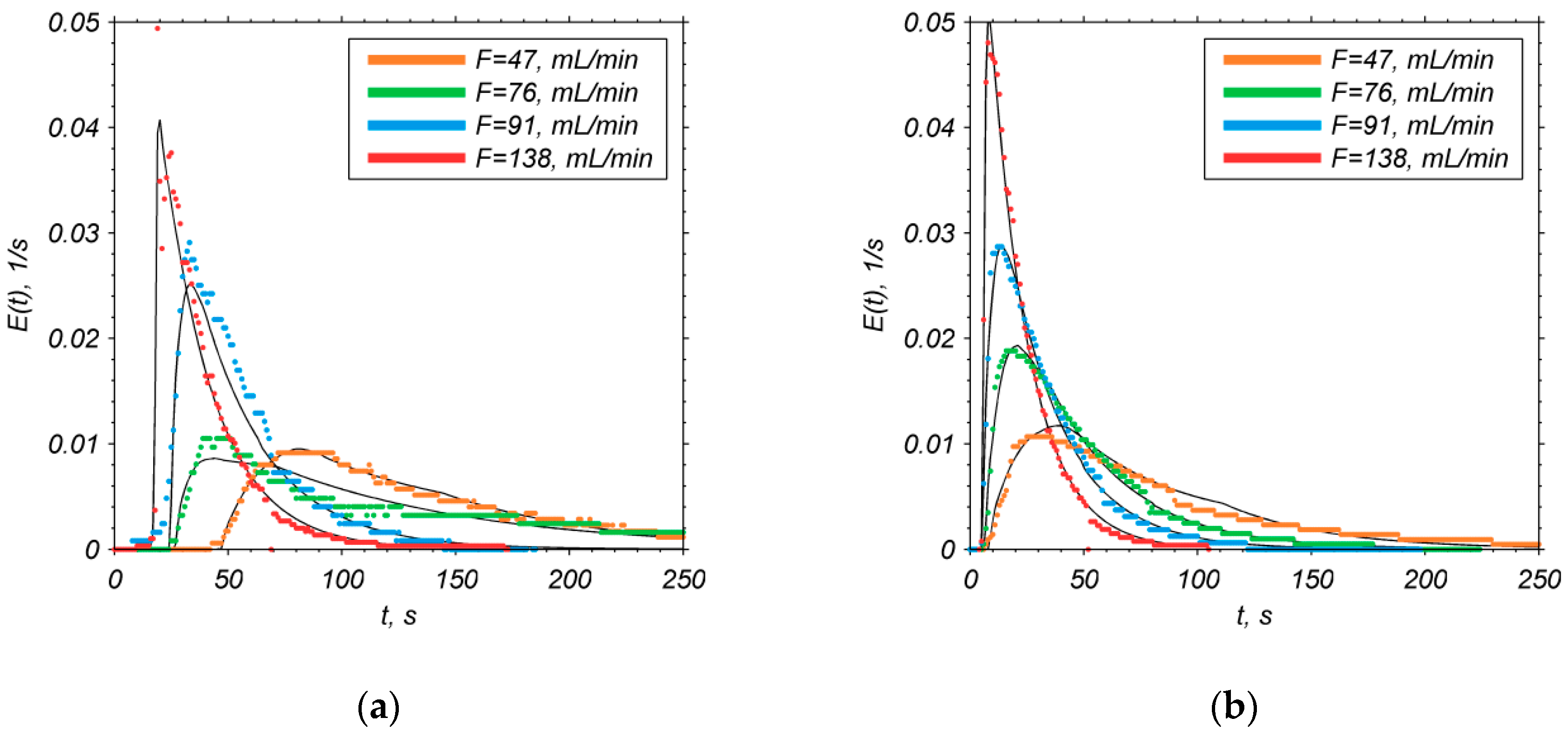
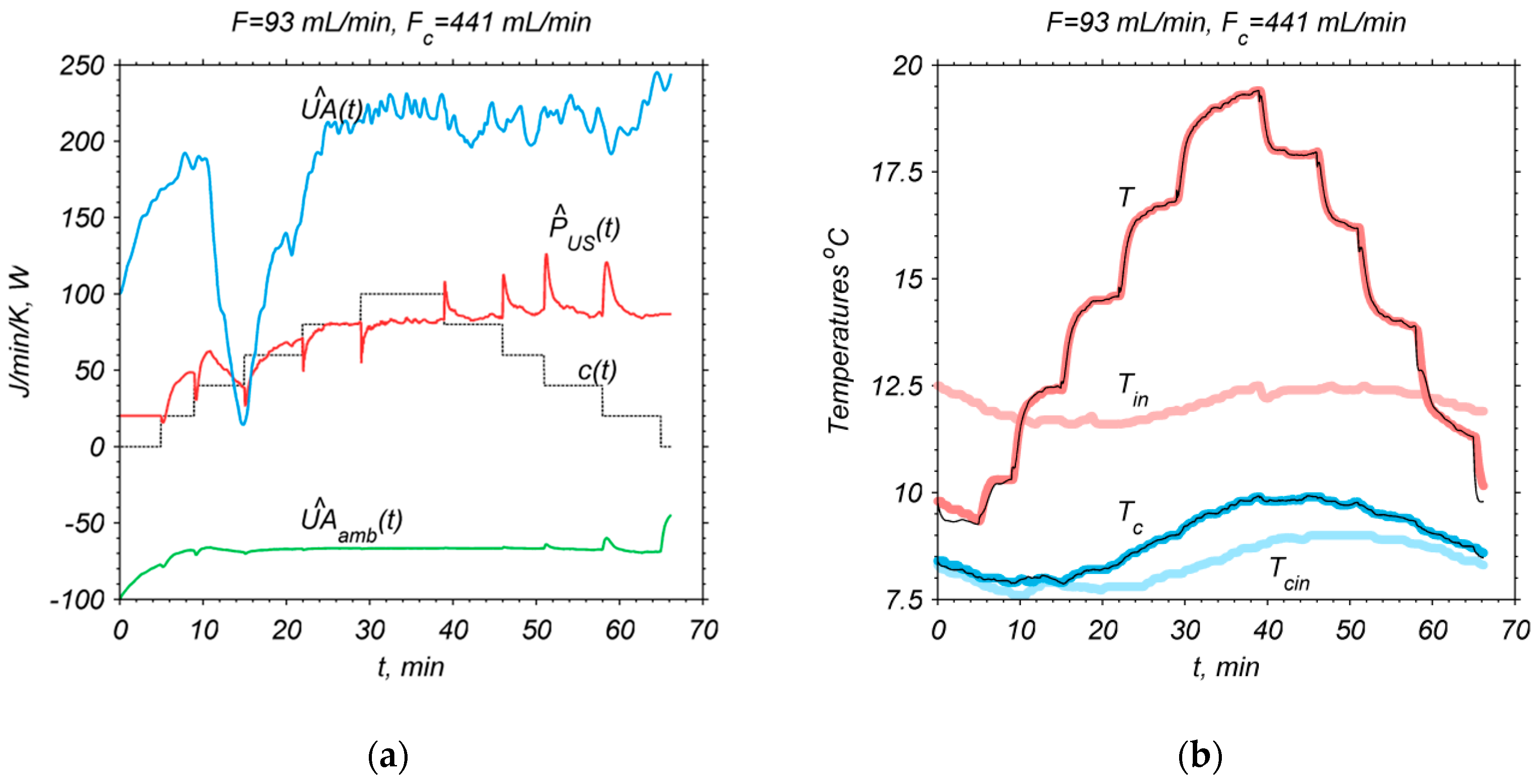
3.3. Experimental Results

The effectiveness of the estimation procedure was tested using results of two experiments carried out for the continuous flow sonochemical reactor depicted in Figure 1. During both experiments, the flow rate through cooling jacket, F_c, was kept constant at F_c = 441 mL/min. The ultrasonic power c(t)P_US was changed in a stepwise manner, where P_US is the maximum ultrasonic power. First, the ultrasonic power was increased from zero to its maximum value P_US by increasing the duty cycle c(t) from 0% to 100% by 20% every few minutes. Then, the duty cycle c(t) was decreased, also in a stepwise manner like before by 20%, and finally to zero. Results of both experiments are presented on Figure 4; Figure 5 for constant flow rates through the reactor F = 93 mL/min or F = 69 mL/min, respectively. The estimates of unknown model parameters $\hat{\theta }$: ${\hat{P}}_{US}(t)$, $U{\hat{A}}_{amb}(t)$, and $U\hat{A}(t)$ are obtained by numerical integration of (6) and (7) for K = 100, Q = 100KI₂, A_F = –50I₂, P = KI₂, Λ = diag(5·10⁵,50,30), $\hat{\theta }(0)={[\begin{array}{ccc}20& -100& 100\end{array}]}^T$(the same in both experiments), and the sampling time T_s = 1 s. Since the state vector is known, the initial conditions in (6) are $\hat{T}(0)=T(0)$, ${\hat{T}}_c(0)=T_c(0)$.

Figure 4b and Figure 5b show the corresponding simulation results for model (3) and (4) by substituting the estimates ${\hat{P}}_{US}(t)$, $U{\hat{A}}_{amb}(t)$, and $U\hat{A}(t)$ into unknown model parameters P_US, UA_amb, and UA, respectively. The model Equations (3) and (4) are solved on-line by using explicit Euler’s method and the vector of estimates $\hat{\theta }(t)$ updated by the observer (6) and (7) every sampling period T_s.

4. Discussion and Concluding Remarks

As shown in Figure 4; Figure 5, the estimated maximum ultrasonic power is not constant and may slightly vary in time. In both experiments for different flow rates F, one can notice a very good agreement (Figure 4b and Figure 5b) between the experimental results and the model (3) and (4) predictions for the vector of estimates $\hat{\theta }(t)$. Hence, one can first perform a preliminary identification experiment to tune the observer (6) and (7) and to find the estimate $\hat{\theta }(t)$. Then, the unknown model parameters in (3) and (4) are updated in the normal operation of the sonochemical reactor, when the ultrasounds are switched on and off. By using the first set of the experimental data (Figure 4), it was possible to tune the observer (6) and (7). According to Equations (8) and (9), the convergence rates of state and parameter errors: $e_x=\widehat{x}-x$, $e_{\theta }=\hat{\theta }-\theta$ are dependent on the observer parameters. By increasing the observer gain K or the absolute values of elements of diagonal matrices A_F and Λ, the convergence rates can be significantly increased. On the other hand, by increasing these values, the observer is more sensitive to measurement noises, and even slight changes in the measured temperatures may lead to significant changes in the estimates, as it can be noticed for $U\hat{A}(t)$ in Figure 4a. A closer look at the estimates in Figure 4a and Figure 5a shows that all the estimated parameters are not constant and may vary. There might be many reasons for this variability, including: amplification of the measurement noises or the non-stationary character of the sonochemical reactor (e.g., the effect of temperature or, in the long run, cavitation erosion of the ultrasonic horn tip). However, in spite of the changes in $\hat{\theta }(t)$, the differences between the simulated and the measured temperatures are minimal (Figure 4b and Figure 5b).

As mentioned earlier, one of the problems with using the observer (6) and (7) is to ensure that the input signals of the identified system are sufficiently exciting [27]. Numerical simulations of the sonoreactor model (3) and (4) have shown that if the ultrasonic power is changed in a stepwise manner (e.g., it is switched on and off), then the estimates converge to true values (Figure 3). The experimental results also showed that step changes in the ultrasonic power ensured the convergence of estimates. Therefore, in the case of batch reactors that are operated at steady-state conditions in continuous (non-pulsed) mode, the system may not be sufficiently excited and the estimates may converge to wrong values. In that case, other methods (e.g., recursive least squares method) may be more suitable.

By using the observer Equations (6) and (7), the ultrasonic power can be easily monitored on-line in the pulse mode. Then, it is possible to design a controller that stabilizes the estimated ultrasonic power at the desired level P_sp, also in the presence of disturbances. A possible structure of the control system is shown in Figure 6. The observer estimates the ultrasonic power $c(t){\hat{P}}_{US}(t)$ and the controller manipulates the duty cycle c(t) to minimize the control error e(t), i.e., the difference between the setpoint P_sp and the estimated ultrasonic power $c(t){\hat{P}}_{US}(t)$. Since there is a very good agreement between the measured temperatures and the model (3) and (4) predictions, advanced control algorithms (e.g., model-based controllers [28,29]) can also be considered. However, in this case, for the proposed estimation method, we must also ensure that the control signal c(t) is sufficiently exciting. This problem will be explored in our future studies.

References

1. Babajide, O.; Petrik, L.; Amigun, B.; Ameer, F. Low-Cost Feedstock Conversion to Biodiesel via Ultrasound Technology. Energies 2009, 3, 1691–1703. [Google Scholar] [CrossRef] [Green Version]
2. Panda, D.; Manickam, S. Cavitation Technology—The Future of Greener Extraction Method: A Review of the Extraction of Natural Products and Process Intensification Mechanism and Perspectives. Appl. Sci. 2019, 9, 766. [Google Scholar] [CrossRef] [Green Version]
3. Subhedar, P.B.; Gogate, P.R. Intensification of Enzymatic Hydrolysis of Lignocellulose Using Ultrasound for Efficient Bioethanol Production: A Review. Ind. Eng. Chem. Res. 2013, 52, 11816–11828. [Google Scholar] [CrossRef]
4. Kandasamy, M.; Hamawand, I.; Bowtell, L.; Seneweera, S.; Chakrabarty, S.; Yusaf, T.; Shakoor, Z.; Algayyim, S.J.M.; Eberhard, F. Investigation of Ethanol Production Potential from Lignocellulosic Material without Enzymatic Hydrolysis Using the Ultrasound Technique. Energies 2017, 10, 62. [Google Scholar] [CrossRef] [Green Version]
5. Kadyirov, A.; Karaeva, J. Ultrasonic and Heat Treatment of Crude Oils. Energies 2019, 12, 3084. [Google Scholar] [CrossRef] [Green Version]
6. Gondrexon, N.; Renaudin, V.; Petrier, C.; Boldo, P.; Bernis, A.; Gonthier, Y. Degradation of pentachlorophenol aqueous solutions using a continuous flow ultrasonic reactor: Experimental performance and modelling. Ultrason. Sonochem. 1999, 5, 125–131. [Google Scholar] [CrossRef]
7. Bilek, S.E.; Turantaş, F. Decontamination efficiency of high power ultrasound in the fruit and vegetable industry, a review. Int. J. Food Microbiol. 2013, 166, 155–162. [Google Scholar] [CrossRef] [Green Version]
8. Yang, S.-C.; Lin, H.-C.; Liu, T.-M.; Lu, J.-T.; Hung, W.-T.; Huang, Y.-R.; Tsai, Y.-C.; Kao, C.-L.; Chen, S.-Y.; Sun, C. Efficient Structure Resonance Energy Transfer from Microwaves to Confined Acoustic Vibrations in Viruses. Sci. Rep. 2016, 5, 18030. [Google Scholar] [CrossRef] [Green Version]
9. Cintas, P.; Mantegna, S.; Gaudino, E.C.; Cravotto, G. A new pilot flow reactor for high-intensity ultrasound irradiation. Application to the synthesis of biodiesel. Ultrason. Sonochem. 2010, 17, 985–989. [Google Scholar] [CrossRef]
10. Rong, L.; Koda, S.; Nomura, H. Study on degradation rate constant of chlorobenzene in aqueous solution using a recycle ultrasonic reactor. J. Chem. Eng. Jpn. 2001, 34, 1040–1044. [Google Scholar] [CrossRef]
11. Gogate, P.R.; Sutkar, V.S.; Pandit, A.B. Sonochemical reactors: Important design and scale up considerations with a special emphasis on heterogeneous systems. Chem. Eng. J. 2011, 166, 1066–1082. [Google Scholar] [CrossRef]
12. Gaudino, E.C.; Carnaroglio, D.; Boffa, L.; Cravotto, G.; Moreira, E.M.; Nunes, M.A.; Dressler, V.L.; Flores, E.M. Efficient H2O2/CH3COOH oxidative desulfurization/denitrification of liquid fuels in sonochemical flow-reactors. Ultrason. Sonochem. 2014, 21, 283–288. [Google Scholar] [CrossRef] [PubMed]
13. De La Rochebrochard, S.; Suptil, J.; Blais, J.F.; Naffrechoux, E. Sonochemical efficiency dependence on liquid height and frequency in an improved sonochemical reactor. Ultrason. Sonochem. 2012, 19, 280–285. [Google Scholar] [CrossRef]
14. Gogate, P.R.; Wilhelm, A.M.; Pandit, A.B. Some aspects of the design of sonochemical reactors. Ultrason. Sonochem. 2003, 10, 325–330. [Google Scholar] [CrossRef]
15. Meng, Z.; Zhou, Z.; Zheng, D.; Liu, L.; Dong, J.; Yang, Y.; Li, X.; Zhang, T. Optimizing dewaterability of drinking water treatment sludge by ultrasound treatment: Correlations to sludge physicochemical properties. Ultrason. Sonochem. 2018, 45, 95–105. [Google Scholar] [CrossRef]
16. Yamaguchi, T.; Nomura, M.; Matsuoka, T.; Koda, S. Effects of frequency and power of ultrasound on the size reduction of liposome. Chem. Phys. Lipids 2009, 160, 58–62. [Google Scholar] [CrossRef] [PubMed]
17. Kimura, T.; Sakamoto, T.; Leveque, J.M.; Sohmiya, H.; Fujita, M.; Ikeda, S.; Ando, T. Standardization of ultrasonic power for sonochemical reaction. Ultrason. Sonochem. 1996, 3, 157–161. [Google Scholar] [CrossRef]
18. Kikuchi, T.; Uchida, T. Calorimetric method for measuring high ultrasonic power using water as a heating material. J. Phys. Conf. Ser. 2011, 279, 012012. [Google Scholar] [CrossRef]
19. Uchida, T.; Kikuchi, T. Effect of heat generation of ultrasound transducer on ultrasonic power measured by calorimetric method. Jpn. J. Appl. Phys. 2013, 52, 07HC01. [Google Scholar] [CrossRef]
20. Dochain, D. State and parameter estimation in chemical and biochemical processes: A tutorial. J. Process Control 2013, 13, 801–818. [Google Scholar] [CrossRef]
21. Abarbanel, H.D.; Creveling, D.R.; Farsian, R.; Kostuk, M. Dynamical state and parameter estimation. SIAM J. Appl. Dyn. Syst. 2009, 8, 1341–1381. [Google Scholar] [CrossRef]
22. Levenspiel, O. Chemical Reaction Engineering, 3rd ed.; John Wiley & Sons: New York, NY, USA, 1998; pp. 109–110. [Google Scholar]
23. Toson, P.; Doshi, P.; Jajcevic, D. Explicit Residence Time Distribution of a Generalised Cascade of Continuous Stirred Tank Reactors for a Description of Short Recirculation Time (Bypassing). Processes 2019, 7, 615. [Google Scholar] [CrossRef] [Green Version]
24. Monnier, H.; Wilhelm, A.M.; Delmas, H. Effects of ultrasound on micromixing in flow cell. Chem. Eng. Sci. 2000, 55, 4009–4020. [Google Scholar] [CrossRef]
25. Legay, M.; Simony, B.; Boldo, P.; Gondrexon, N.; Person Le, S.; Bontemps, A. Improvement of heat transfer by means of ultrasound: Application to a double-tube heat exchanger. Ultrason. Sonochem. 2012, 19, 1194–1200. [Google Scholar] [CrossRef]
26. Haessig, D.A. On-line State and Parameter Estimationin Nonlinear Systems. Ph.D. Thesis, Science & Technology University, Newark, NJ, USA, May 1999. [Google Scholar]
27. Narendra, K.S.; Annaswamy, A.M. Stable Adaptive Systems; Courier Corporation: North Chelmsford, MA, USA, 2012. [Google Scholar]
28. Tatjewski, P. Offset-free nonlinear Model Predictive Control with state-space process models. Arch. Control Sci. 2017, 27, 595–615. [Google Scholar] [CrossRef] [Green Version]
29. Choinski, D.; Skupin, P.; Krauze, P.; Ilewicz, W.; Bielecki, Z. Isopropanol concentration control in the ultrasonic nebulization process. In Proceedings of the 22nd International Conference on Methods and Models in Automation and Robotics. MMAR 2017, Miedzyzdroje, Poland, 28–31 August 2017; pp. 31–36. [Google Scholar] [CrossRef]
Figure 1. Scheme of the measuring setup for ultrasonic tests.
Energies 13 02952 g001
Figure 2. Exit time distributions in the reactor vessel, when the ultrasounds are: (a) switched off; (b) switched on. Black continuous lines are model responses.
Energies 13 02952 g002
Figure 3. Time courses of estimates of model parameters for different initial conditions θ ^ ( 0 ) for a numerically simulated system.
Energies 13 02952 g003
Figure 4. Experimental results for F = 93 mL/min: (a) estimates of unknown model parameters θ ^ ( t ) = [ P ^ U S ( t ) U A ^ a m b ( t ) U A ^ ( t ) ] T ; (b) measured temperatures (thick red and blue lines) and model predictions (black lines) for θ ^ ( t ) .
Energies 13 02952 g004
Figure 5. Experimental results for F = 69 mL/min: (a) estimates of unknown model parameters θ ^ ( t ) = [ P ^ U S ( t ) U A ^ a m b ( t ) U A ^ ( t ) ] T ; (b) measured temperatures (thick red and blue lines) and model predictions (black lines) for θ ^ ( t ) .
Energies 13 02952 g005
Figure 6. Scheme of the control system for stabilization of the ultrasonic power.
Energies 13 02952 g006