Abstract
The flow of energy within external gear machines (EGMs) leads to the variation of fluid temperature in the EGMs, which affects their performance. However, the common approaches for the simulation of EGMs assume isothermal conditions. This isothermal assumption negatively impacts their modelling accuracy in terms of the internal flows which are dependent on the fluid temperature (via fluid properties). This paper presents a lumped parameter based thermal model of EGMs where the fluid temperature in the EGM is evaluated considering the effects of compression/expansion, internal flows, and power losses. Further, numerical techniques are developed to model each of these three aspects. The thermal model is validated via the outlet temperature and volumetric efficiency measurements obtained from experiments conducted on six units of an EGM taken as a reference with different internal clearances. The results from the model show that the fluid temperature increases as it is carried from the inlet side to the outlet side during the pumping operation. However, the fluid at the ends of the shafts has the highest temperature. By comparing the isothermal simulation results with the proposed thermal model, the results also point out how the isothermal assumption becomes inaccurate, particularly in conditions of low volumetric efficiency.
1. Introduction
External gear machines (EGMs) are positive displacement machines that are used in a variety of applications. The fluid power applications include industrial and mobile equipment. In the automotive/aerospace industry, they are used in fuel injection and lubrication systems. Moreover, they are also used in several fluid handling applications.
In the following paragraphs, a brief description of the EGM operation is reported to: (a) illustrate the geometry of the reference EGM used for the simulation and the experimental activity in this research; (b) familiarize the reader with the nomenclature used by the authors in the paper. Readers interested in a more fundamental description of EGMs are encouraged to refer to specific references, such as [1].
EGMs consist of two meshed gears surrounded by casing and front/end covers (Figure 1). Pressure compensated EGMs [2] also have floating elements (plates or bushings) to control the gaps on the lateral sides of the gears. However, the EGM taken as a reference in this work (Figure 1) is not a pressure compensated design.
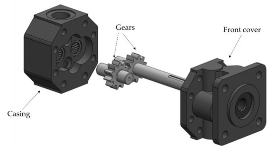
Figure 1.
Reference external gear machine (Concentric GC series pump).
During the rotation of the gears, the volume between the gear teeth (referred to as the tooth space volume, TSV) leaving the meshing zone increases in size, leading to the suction of the operating fluid from the inlet (Figure 2). The fluid is then carried in the TSV from the inlet side to the outlet side. On the outlet side, when the gear teeth enter the meshing zone, the volume of the tooth space decreases, resulting in the delivery of the fluid to the outlet.

Figure 2.
Operation of EGMs and leakage flows. (a) front view, where the color of the fluid volume qualitatively indicates the level of fluid pressure in the pumping action; (b) side view, showing the drain leakage path in the reference EGM.
The operation of EGMs involves relative motion between the gears and the casing/cover. To avoid contact between these parts, the EGMs are manufactured such that there are clearances between them along both the radial and the axial direction. However, these clearances become the source of power losses in the EGMs in the form of leakage flows and friction on the gears’ surfaces.
The clearances allow the working fluid to leak from the high pressure environment to the low pressure one negatively affecting the volumetric performance of the EGMs. Figure 2 shows the three types of leakage flows in the EGMs. The leakage flow between the adjacent TSVs through the clearance at the tooth tip is referred to as the tooth tip leakage. The leakage flow between the adjacent TSVs through the axial gap is referred to as the lateral leakage. The axial gap also allows the fluid to leak from the TSVs to the shafts of the gears. This portion of the leakage is referred to as the drain leakage as this flow is used to flush the bearings that support the shafts. This flow then either exits the EGM via the drain port (typical for hydraulic motors) or flows back to the inlet via an internal drain channel (which is typical for hydraulic pumps). The latter configuration is shown in Figure 2b.
The leakage flows also give rise to the friction forces on the gears’ surfaces. Moreover, as the gears mesh, the relative motion between the teeth surfaces of both results in friction. An extra amount of work is done (by the prime mover in the pumping operation/by the fluid in the motoring operation) to overcome these friction forces. The work done against the friction forces results in the frictional heating and thus, power losses in the EGMs.
These power losses along with the compression of the fluid (in pumping operation) lead to the rise of the temperature of the working fluid. The fluid temperature is a critical parameter in the EGM operation. The viscosity of the working fluids (which influences the leakage flows and friction) highly depends on temperature (Figure 3). Thus, the overall performance of EGM is dependent on the fluid temperature.
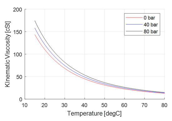
Figure 3.
Effect of temperature on viscosity for the fluid taken as reference in this research (ISO VG 46 mineral oil).
Simulation models are efficient tools for analyzing the operation of EGMs and predicting their performance. Moreover, they can also be used for design purposes. Considering the importance of the fluid temperature, to accurately predict the performance of EGMs, the simulation models for EGMs should include methods to evaluate the fluid temperature in the EGMs and model its effect.
Apart from the performance of the EGMs, the temperature of the outlet flow of the EGMs can also be critical for the performance of other hydraulic components in the circuit downstream of it. Thus, it is desirable for the EGM simulation models to predict the outlet temperature.
Researchers in the past have developed several simulation models for analyzing the fluid displacing action in EGMs and predicting their performance. Theoretical models for the analysis of the ideal flow behavior of EGMs were developed by Bonacini [3], Ivantysyn and Ivantysynova [1], and Manring and Kasaragadda [4]. Simulation models based on a lumped parameter approach were developed by Manco and Nervegna [5], Eaton et al. [6], and Zardin et al. [7] with the focus on the prediction of pressure in the TSVs. These models, however, did not consider aspects related to gear micromotion, which is a key phenomenon impacting the performance of EGMs.
In EGMs, due to the difference in pressure at the inlet and outlet ports, the gears are subject to radial forces. In response to these forces, the clearances between the gear shafts and the bearings supporting them allow changes in the radial position of the gears of the order of few microns. This micromotion influences the gap heights at the tooth tips of the gears which, in turn, affects the leakage flows and friction forces at the tooth tips.
Lumped parameter based models have a critical advantage that they can be easily integrated with mechanical models for the evaluation of gear micromotion. Such integrated simulation models have been developed by Zardin and Borghi [8], Falfari and Pelloni [9], and Mucchi et al. [10]. In the past decade, the authors’ research group has developed their own EGM simulation tool, HYGESim (hydraulic gear machine simulator) [11]. An active coupling between the lumped parameter-based fluid model and the mechanical model has allowed this tool to accurately predict the TSV pressures, outlet flow, and gear micromotion. Further, the computational swiftness of this tool has allowed it to be used in the optimization studies to develop novel gear designs [12,13].
In recent years, CFD (computational fluid dynamics) based methods for the modelling of EGMs have become popular [14,15,16]. However, compared to the lumped parameter based methods, they have two crucial downsides. First, they are computationally expensive, rendering them unsuitable for design optimization algorithms. Second, they do not consider the effects of gear micromotion.
With respect to the fluid temperature in EGMs, a key limitation of the past EGM simulation models is that they assume isothermal flow conditions in EGMs. To improve the accuracy of the results obtained from the model, these isothermal models can be run using the mean value for the temperatures at the inlet and the outlet ports of the EGM. However, this port temperature information needs to be known from the experiments. This dependence on the experimental data hampers the predictive capability of the simulation models. Further, the isothermal models cannot predict the effects of viscosity variations with temperature of the internal gap flows of Figure 2, which affects the unit efficiency.
The first research work that involved the port temperatures of EGMs was related to the development of the thermodynamic model for the prediction of pump efficiency based on the port pressure and temperature measurements by Manco and Nervegna [17]. Similar models have been developed in recent years by Lana and De Negri [18] and Casoli et al. [19] (the latter was focused on axial piston pumps). These models, however, are not predictive as they rely on the outlet temperature measurements. Efforts towards the development of thermal models that can allow the prediction of the outlet temperatures have been made by Zecchi et al. [20] and Shang and Ivantysynova [21] for axial piston machines. For EGMs, the thermal effects have been considered in the modelling of the axial balance of floating elements in pressure compensated units [22,23]. However, this approach too requires accurate temperature information from the lumped volumes of the EGM which cannot be provided by the state-of-the-art EGM simulation models.
The goal of the work presented in this paper is to overcome the aforementioned limitations of past simulation models by developing a thermal model of EGMs based on the lumped parameter approach. The model uses fundamental equations of thermodynamics, applied to the lumped elements (control volume and volume connections) with an approach that is also similar to what is applied within the simulation tool Simcenter Amesim [24]. However, the application of such approach to interpret the thermal effects affecting EGM operation is for the first time presented in this work. The thermal model here developed is integrated with the EGM simulation tool HYGESim. This integrated model is referred to as “thermal-HYGESim” in the paper. The model is able to predict the temperature in all the control volumes (CVs) of the EGM including the temperature at the outlet. The instantaneous temperature information is used to update the local fluid properties in the CVs, hence permitting an accurate evaluation of internal flows and thus, the overall performance of EGMs.
The model developed in this work is validated via the outlet temperature and volumetric efficiency measurements from the flow experiments conducted on the reference EGM. The reference EGM considered in this work is the concentric GC series external gear pump [25]. The geometric details of the EGM are provided in Table 1.

Table 1.
Geometric parameters of Concentric GC series pump (used as reference in this work).
The paper is structured into four sections including this introductory section. In Section 2, the numerical approach of the thermal-HYGESim model is described in detail. In Section 3, key results from the model are presented and the comparisons with experimental results are shown. Finally, major conclusions of the paper are provided in Section 4.
2. Thermal-HYGESim Model
This section provides a description of the thermal-HYGESim model. It includes a brief outline of the original HYGESim model developed at the Maha Fluid Power Research Center of Purdue University with a detailed description of the thermal aspects developed in this work. A comprehensive description of the original isothermal version of the HYGESim model can be found in [11].
The thermal-HYGESim model consists of multiple interconnected modules as shown in Figure 4. Among them, fluid dynamic module, loading module, micromotion module and geometrical module are the ones relevant to this work. In the following subsections, the details of these modules are described.

Figure 4.
Modules in HYGESim tool.
2.1. Fluid Dynamic Module
The fluid dynamic module is the central module of thermal-HYGESim. It is based on the lumped parameter approach where the fluid domain in the EGM is divided into several control volumes. Referring to Figure 2, the TSVs of the drive gear () and driven gear (), the volumes on the inlet side () and outlet side () and the drain volume () are considered as distinct CVs. The fluid properties in these CVs (pressure, temperature, density, bulk modulus, viscosity, specific heat, thermal expansion coefficient, and specific heat) are assumed to be spatially uniform and are only a function of time.
2.1.1. Pressure and Temperature Evaluation in CVs
The governing equations for the pressure and temperature in the CVs can be derived from the laws of conservation of mass and energy, respectively. Figure 5 shows a generic CV. The CV has number of ports via which the exchange of mass (mass flow rate ) and energy (enthalpy flow rate ) occurs. Moreover, the volume of the CV varies with the rate of .
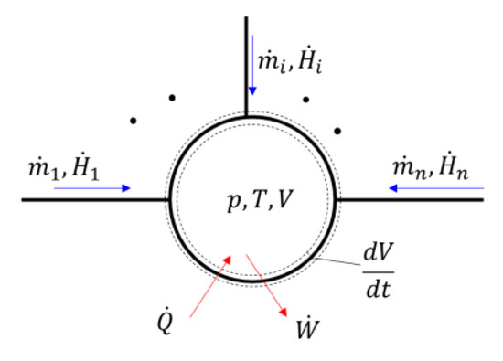
Figure 5.
Schematic of a typical CV in EGM with number of ports and varying volume.
The governing equation for pressure in the CV (referred to as the thermal pressure build up equation) is
The three terms in this equation represent the rise of pressure in the CV due to the fluid inflow, the reduction of the volume of the CV and the increase of the fluid temperature.
The governing equation for temperature in the CV (referred to as the temperature rise equation) is
In this equation, the first term represents the rise of temperature in the CV from heat inflow. For the CVs in EGMs, this represents the frictional heating. The second term represents the rise of temperature due to the inflow/outflow at the ports of the CV. In particular,
Thus, this term accounts for the rise/fall in the temperature of the fluid in the CV due to the difference in the specific enthalpy of the fluid entering the CV and the fluid in the CV. The last term in Equation (2) accounts for the effect of compression/expansion of the fluid on the fluid temperature in the CV.
The derivation of the thermal pressure build-up and temperature rise Equations (1) and (2) suitable for lumped parameter modeling of fluid systems is hard to find in the literature. Therefore, the authors decided to provide the details of their derivation in Appendix A and Appendix B.
It is notable that the fluid properties () used in the model are the functions of pressure and temperature. Thus, the pressure and temperature values determined from Equations (1) and (2) are used to update these fluid properties in the simulation model.
2.1.2. Mass Flow between the CVs
In the lumped parameter approach, the flow connections between the CVs are modelled as hydraulic resistors. Figure 6 shows the schematic of a hydraulic resistor connecting two CVs.
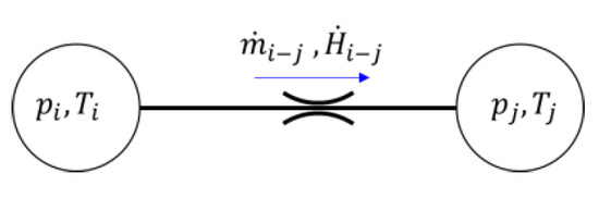
Figure 6.
Schematic of a hydraulic resistor connecting two lumped volumes at pressures and and temperatures and .
The hydraulic resistors between the TSVs and the inlet/outlet volumes are modelled using the turbulent orifice equation:
Here, is the orifice flow coefficient which is dependent on the flow Reynolds number [26].
The hydraulic resistors between the adjacent TSVs allow the tooth tip and lateral leakage flows. These flows are driven by the pressure difference between the adjacent TSVs and the relative motion of the tooth with respect to the casing/cover. Thus, these flows are modelled using the combined Couette–Poiseuille equation:
where is the height of the gap. It is to be noted that, to differentiate between the specific enthalpy and gap height, the authors use the symbol to denote the specific enthalpy and to denote the gap height.
The hydraulic resistor between the TSVs and the drain volume allows the drain leakage flow. This flow is only driven by the pressure difference and thus is modelled using the plane Poiseuille equation (Equation (5) with ). For the EGMs with internal drains, the fluid from the drain volume flows to the inlet via circular internal channels. An example of such a channel is shown in Figure 2b. The flow through such channels are modelled using Hagen–Poiseuille equation.
2.1.3. Enthalpy Flow between the CVs
The fluid flowing through a hydraulic resistor has the enthalpy of the upstream CV. Thus, the enthalpy flow rate associated with the mass flow through this resistor is calculated as:
where the specific enthalpy, , is evaluated at the pressure and temperature of the upstream CV. The assumption associated with this relation is that there is no heat gain/loss to the environment in this flow. The validity of this assumption is presented in Section 3.3 where it is shown that the heat transfer to the environment is negligible compared to the magnitude of enthalpy flows.
2.2. Loading and Gear Micromotion Module
The fluid pressure in the TSVs and the friction forces on the gears’ surfaces induce radial forces and axial moments on the gears. The techniques for the evaluation of forces and moments from different sources are described in the following subsections.
2.2.1. Effect of Fluid Pressure
The evaluation of the forces and moments arising from the fluid pressure is already present in the original HYGESIM tool and the detailed approach is described in [11]. In this subsection, a brief summary of the approach is reported.
The pressure forces acting on each tooth space () are calculated by evaluating the product of the pressure inside the TSV and projection of the tooth space area in the Cartesian directions (Figure 7). The projection area information is provided by the geometrical module (described in Section 2.3). The net radial force from pressure on each gear is

Figure 7.
Forces acting on the gears. Force from fluid pressure on one TSV is shown: and are the forces and and are the projection areas of the TSV in the cartesian directions. and are contact and friction forces, respectively.
From the information about the individual forces from fluid pressure and their line of action ((), obtained from the geometrical module), the pressure moment acting on each gear is calculated as:
2.2.2. Effect of Friction at the Tooth Tip
The friction force on the gears’ tooth tips and lateral surfaces are evaluated by integrating the shear stress exerted on these surfaces by the leakage flows. For the Couette–Poiseuille flows, the shear stress is expressed as:
For tooth tip (Figure 8), this expression simplifies to

Figure 8.
Gap at the tooth tip.
From the shear stress expression, the friction force can be calculated as
Finally, the friction moment on the gear is
2.2.3. Effect of Friction at the Lateral Leakage Interface
For the lateral leakage interface, the shear stress expression for a differential slice of tooth shown in Figure 9 is
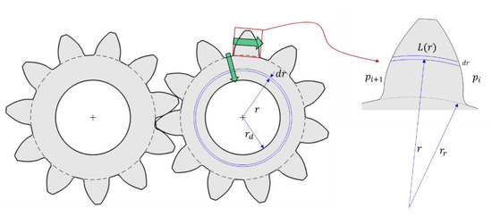
Figure 9.
Differential slices for the evaluation of shear stresses in lateral leakage and drain leakage interfaces. Green arrows show the flow directions.
It is to be noted that the length of the gap varies with distance of the slice from the gear center. Thus, the friction force acting over one tooth is
and the friction moment from the shear stress on one tooth is
The integrals in Equations (14) and (15) are geometric quantities and thus can be determined for any given gear geometry.
2.2.4. Effect of Friction at the Drain Leakage Interface
In the drain leakage interface, the pressure driven leakage flow is along the radial direction (Figure 9). Thus, the shear stress due to this flow does not generate any friction moment. The friction moment only occurs due to the Couette flow arising from the relative motion of the gear with respect to the casing/cover. Thus, the shear stress expression for a differential slice is simply
Due to the radial symmetry, the net friction force on the drain interface is zero. The friction moment acting on this interface is
2.2.5. Contact and Friction Force at the Meshing Interface
The net moment on each gear is the sum of the pressure moment and the friction moments.
The moment on the driven gear is balanced by the moment due to the contact force between the gears acting along the line of action. The expression of contact force is
where is the radius of the pitch circle and is the pressure angle of the gear. The friction force at the contact point (referred to as the meshing friction) can be determined as
where is the friction coefficient obtained from the relation proposed by Jacobson and Hamrock [27] for line EHL contacts. The usage of EHL friction relation is appropriate since the contact forces in EGMs are of the order of few kilonewtons. Such forces acting over a small region of meshing contact result in the elastic deformation of the contact surfaces. Thus, the condition of elastohydrodynamic lubrication (EHL) exists at these surfaces.
The friction moment on the gears due to the meshing friction force can be determined as:
where is the length of the moment arm (shown in Figure 7).
2.2.6. Power Losses Due to Friction
From the friction moment expressions (Equations (12), (15), (17), and (21)), the power losses can be evaluated as the product of the friction moment and shaft speed.
Another source of power loss in the EGMs is the bearings. The reference EGM consists of needle bearings for which power loss relation proposed by Trippett [28] is used. The power losses in the EGM are converted into heat, raising the fluid temperature in the EGM. This heating is accounted in the temperature rise equation via the term.
The techniques for modelling the friction presented in the previous sections have been validated by the authors, the details of which will be discussed in a future work.
2.2.7. Gear Micromotion
The radial forces acting on the gears push the gears towards the low pressure side of the EGM. For the EGMs with journal bearings, the magnitude and direction of the radial motion of the gears (gear micromotion) is obtained from the mobility solution of journal bearings [29]. For the EGMs with needle bearings, the magnitude of micromotion is considered to be equal to the clearance between the shafts and the bearings. Moreover, the direction of micromotion is considered to be the same as the direction of the radial force.
2.3. Geometrical Module
The geometrical module takes the geometric parameters of the EGM as inputs and provides the information about the geometric features relevant to other modules in HYGESim. The inputs are in forms of either the CAD drawings or the parametrized data. A key input is the instantaneous position of the gears in the casing which is affected by the micromotion of the gears.
The module implements an algorithm to divide the fluid domain into distinct CVs. It evaluates the volumes of all the CVs and the areas of all the flow connections. This information is passed to the Fluid Dynamic Module. Next, it evaluates the projection areas of TSVs ( and in Figure 7) and distance of their centroids from the axis ( in Figure 7). This information is provided to the loading module. A detailed description of the algorithm implemented in the geometrical module is present in [30].
This completes the description of the relevant modules in thermal-HYGESim and approaches within them. Lastly, the authors want to point out that, in this work, the effect of differential thermal dilatation of the solid material is not considered. However, this is a good approximation for the reference unit which uses a similar material (from the point of view of thermal expansion coefficient) for the gears and the casing.
3. Results and Experimental Validation
The thermal-HYGESim model described in Section 2 is used to simulate the operation of the reference EGM (presented in Section 1). In this section, the results obtained from the simulations are described and are compared against the experimental data. A comparison is also made with the traditional isothermal HYGESim model to highlight the significance of the proposed thermal-HYGESim model.
3.1. Simulation Setup
Figure 10 shows the hydraulic circuit simulated in thermal-HYGESim. The circuit reproduces the experimental set up considered in this research, which is described in Section 3.4. The pressure boundary conditions for the pump being simulated is 0 bar at the inlet tank and at the outlet port. The fluid temperature at the inlet tank is set to . The initial temperature and pressure of the fluid in the pump are set to and 0 bar respectively.

Figure 10.
Hydraulic circuit simulated in thermal-HYGESim.
In the simulations, an assumption related to the axial location of the gears in the EGM cavity needs to be made. This decides the height of the axial gap on each side of the gears. In the reference unit, the geometry is symmetric on both sides of the gears. However, micron level deviations on the planarity of the axial surfaces of the gears, casing, and front cover might be present. This may generate hydrodynamic effects resulting in axial forces on both the gears. The authors’ research center has observed this effect on gerotors, as documented in [31]. However, in EGMs, due to the presence of two gears with opposite direction of rotation, such axial forces can have a canceling effect (depending on the machining tolerance). Thus, in this work, the gears are considered to be symmetrically placed in the EGM cavity.
3.2. Key Results from Thermal-HYGESim Model
This subsection describes the key results obtained from the simulation of the reference EGM using the thermal-HYGESim model. Figure 11 shows that the fluid temperature the inlet (), outlet () and drain () volumes of the pump are higher than their initial temperature and the temperature of the inlet tank (). These temperatures increase with pressure which is expected due to the increase in power losses with pressure. Among all the volumes, the drain volume has the highest temperature. increases (from its initial temperature) as the drain volume collects high enthalpy drain leakage flows from the TSVs. increases as it receives high enthalpy flows from the tooth tip and lateral leakage interfaces as well as the flow from the drain volume. However, is lower than others as the majority of the flow entering the inlet volume is the low enthalpy flow from the inlet port of the pump. Finally, increases due to the high enthalpy flows delivered by the TSVs.

Figure 11.
Temperatures at the inlet, outlet and drain CVs of the EGM obtained from the simulation setup in Figure 10 with rpm.
Figure 12a shows the variation of pressure and temperature in a drive gear TSV for two shaft revolutions. The angular position convention used in this figure is the same as shown in Figure 1.

Figure 12.
(a) Pressure and temperature variation in a TSV of the drive gear over two shaft revolutions; (b) Gap height over the tip of the leading tooth of a TSV of the drive gear. For and , the tooth tip does not form a leakage interface with the casing, so, the gap height is not defined for that range.
As the TSV, , enters the casing (i.e., both the leading and lagging tooth tips of the TSV form leakage interfaces with the casing), the leakage flow from the leading TSV, , via the gaps at the tooth tip and the lateral sides of the gear, pressurizes the fluid in the TSV, . The course of pressurization from bar to bar follows a non-linear behavior due to non-uniform gap height at the tooth tip (Figure 12b). The change in this gap height is a direct consequence of gear micromotion, where the gear moves towards the low pressure side, decreasing the tooth tip gap height near and increasing the gap height near . At , a jump in TSV pressure is observed. This is associated with the sudden opening of the TSV to the outlet volume when the leading tooth leaves the casing (i.e., the tooth tip no longer forms a leakage interface with the casing). This jump induces similar (although low magnitude) jumps in the lagging TSVs which is observable in the pressure plot for .
During the pressurization of the TSV, , it receives leakage flows from the leading TSV, . Since the leading TSV, , is at a higher pressure, the leakage flows have higher enthalpies. The high enthalpy inflow combined with the pressurization of the TSV, , results in the increase of the temperature in the TSV, . The trend of the temperature in the TSV stays similar to the pressure trend until the TSV reaches the meshing zone (). This includes the first spike in the TSV temperature at which associated with the compression of the fluid trapped in the TSV upon entering the meshing zone.
After , a second spike in the TSV temperature is observed. This spike is caused by two factors:
- Lateral leakage flow from the lagging TSV, i.e., from to in Figure 13c. The fluid in has higher pressure and temperature, and thus, has higher specific enthalpy as compared to the fluid in . Thus, the lateral leakage flow carries the high specific enthalpy fluid to a low specific enthalpy environment raising the temperature of the latter. This effect is mathematically captured by the terms in the temperature rise equation (Equation (2)). From Figure 13b, the leakage enthalpy flow is higher than the product of the specific enthalpy of the fluid in and the leakage mass flow rate (). Thus, the aforementioned terms in the temperature rise equation yield a positive value promoting .
 Figure 13. (a) TSV temperature in the meshing region; (b) Plot of different terms in the temperature rise equation (Equation (2)). and are the leakage enthalpy and mass flow rates, respectively, from to . is the specific enthalpy of the fluid in ; (c) Illustration of the lateral leakage flow (green arrow) from TSV, , to the TSV under investigation, . The color of CVs are the qualitative indicators of the fluid pressure.
 - Friction heating due to the meshing of the gear teeth (black curve in Figure 13b). In the temperature rise equation (Equation (2)), this factor appears as a positive promoting .
3.3. Heat Loss to the Environment
Researchers in the past have commented that, during the operation of EGMs, the heat transfer to the environment is negligible compared to the energy flow in the EGM [18,19]. However, to confirm this theory for the reference EGM, a simple steady state thermal analysis of the EGM casing was conducted in ANSYS Mechanical [32].
Figure 14a shows the CAD of the solid bodies used in the thermal analysis. The bodies include the mounting plate used to mount the reference EGM on the test rig during the experiments (details in Section 3.4). Including the mounting plate is important as it provides a higher surface area for the free convection of heat. For simplicity, the fluid in the interior of the pump was assumed to be at the temperature of , which is the highest temperature in the internal CVs observed in the simulations. The air temperature around the casing and the mounting plate was assumed to be (lower end of the room temperature range). Thus, these boundary conditions act as the upper bound (or the worst case scenario) for the heat loss to the environment.
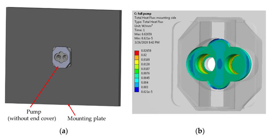
Figure 14.
(a) CAD of the reference EGM (end cover removed to show the interior domain) and the mounting plate used in the steady state thermal analysis. (b) Heat flux at the interior surfaces obtained from the results of thermal simulation in ANSYS.
The results from this thermal analysis confirm that the heat flux to the environment from the interior surfaces of the EGM (Figure 14b) is indeed much lower than the rate of energy flow in the EGM. For instance, the radial heat flux from the internal periphery of the casing is W/mm2 W. This is negligible compared to the circumferential enthalpy flow watts (at rpm). Similarly, the heat flux in the axial direction (at the lateral lubrication interface) is W/mm2. Thus, the heat losses over the area of lateral and drain leakage interface (for single tooth) are W and W, respectively. These values are insignificant compared to the levels of enthalpy flow rates at these interfaces (Figure 15).
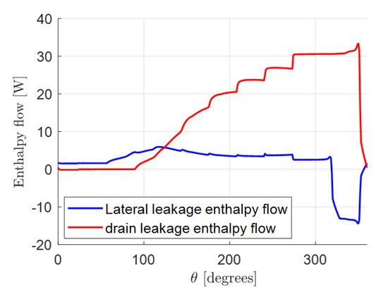
Figure 15.
Enthalpy flow rates at the lateral and drain leakage interfaces for one tooth over its full revolution. The results are obtained from the simulation of the reference EGM at rpm, bar, .
From these results, it is concluded that, for the reference EGM, the heat loss to the environment is inconsequential in its thermal analysis and thus is neglected in the thermal-HYGESim model.
3.4. Experimental Validation of Thermal-HYGESim Model
One of the main capabilities of the thermal-HYGESim model developed in this work is the prediction of the temperature at the outlet of the EGM. Moreover, the fluid temperature predicted inside the EGM influences the leakage flows and thus, the outlet flow. Hence, for the validation of thermal-HYGESim model, an experimental setup was designed to run flow experiments on the reference EGM and measure the outlet temperature and the outlet flow for a range of operating conditions.
Figure 16 shows the ISO schematic of the hydraulic circuit. The electric motor drives the pump (reference EGM) which draws the fluid from the tank and pushes it through a needle valve (represented by the variable orifice in the figure). Pressure transducers, a flow sensor, and thermocouples are mounted on the hydraulic line to record the pressures, flow rate and temperatures, respectively, at different locations. The details of the sensors are present in Table 2. Figure 17 shows the picture of the actual test setup. The experiments were conducted for a range of operating conditions by varying the motor speed (thereby changing the pump speed) and varying the needle valve setting (thereby varying the pressure at the pump outlet). Via the inlet thermocouple, it was ensured that the inlet temperature stayed at 35 °C.

Figure 16.
ISO schematic of the hydraulic circuit used in the experiments.
Table 2.
Details of sensors used in the tests.

Figure 17.
Picture of the test setup (Photographer: Rituraj).
Six units of the reference EGM were tested in this work. The gears in these units suffer from two types of manufacturing errors:
- Conicity error: The surface formed by the tooth tips of the gear is conic instead of cylindrical (Figure 18a).
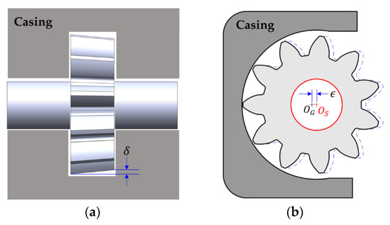 Figure 18. Illustration of (a) conicity error and (b) concentricity error in gears: and are shaft and gear centers respectively.
 - Concentricity error: The gear axis is eccentric with respect to the shaft axis (Figure 18b).
Table 3 summarizes the magnitude of conicity and concentricity errors on the gears of the six units.
Table 3.
Effective gap heights at the tooth tips of the gears in the six units used in the experimental tests.
As illustrated in Figure 18, these manufacturing errors result in non-uniform gap height at the tooth tips of the gears (even after excluding the effects of gear micromotion). Detailed methodology for including the effects of these errors in the simulation model can be found in [33]. However, to aid the interpretation of results shown later, the effective gap height information is provided for each unit in Table 3. For gears with aforementioned manufacturing errors, an effective gap height at the tooth tip can be defined such that an EGM with ideal gears (no manufacturing errors) and this effective gap height will exhibit same volumetric performance as an EGM with real gears (which have these manufacturing errors). In other words, the effective gap height accounts for the effects of these manufacturing errors. The technique for the evaluation of this effective gap height is present in [33].
The results obtained from the simulations and experiments for all the units are shown in Figure 19 (volumetric efficiency) and Figure 20 (outlet temperature). The trends in each of the plots can be understood by considering the effects of speed and pressure on the leakage flows and the effects of leakage flows on the volumetric efficiency and outlet temperature. The leakage flow increases with pressure and decreases with speed. Higher leakage flow is directly related to a lower volumetric efficiency. Moreover, power loss from the leakage flow raises the temperature in the unit which is reflected in a higher outlet temperature.

Figure 19.
Comparison of the volumetric efficiency predicted by the simulations (Thermal HYGESim and traditional isothermal HYGESim) and evaluated from flow measurements in the experiments for all six units.

Figure 20.
Comparison of the outlet temperature predicted by the simulations and the outlet temperature measured in the experiments for all six units.
The variation of results across the units can be explained from the fact that the tooth tip leakage flow is directly dependent on the effective gap height. As the effective gap height is the lowest for unit 6 (among all the units), the tooth tip leakage flow is the lowest, resulting in the volumetric efficiency being the highest and the outlet temperature being the lowest. Vice versa is true for unit 3.
In Figure 19 and Figure 20, a good match between the simulations and experiments is observed in terms of both the volumetric efficiency and the outlet temperatures. The performance of the thermal-HYGESim model can be analyzed by defining the model error with respect to the volumetric efficiency prediction as . The mean efficiency error obtained from all the simulations shown in Figure 19 is 1.57 %. Further, the model error in terms of the outlet temperature prediction is defined as . The mean error of temperature prediction by the thermal-HYGESim model for the simulations in Figure 20 is .
In Figure 19, the simulation results from the traditional isothermal-HYGESim model is also presented. For obtaining these results, the (constant) temperature of simulations is set to the mean of the inlet and outlet temperatures observed in the experiments. Qualitatively, it is observed that the isothermal-HYGESim model predicts a higher efficiency compared to the proposed thermal-HYGESim model. This difference is small at high efficiency conditions, but it gets magnified at lower efficiency conditions. In other words, the isothermal model’s accuracy suffers at lower efficiency conditions. This is further discussed in Section 3.5. Quantitatively, the mean efficiency error of the isothermal model for the simulations shown in Figure 19 is 2.40%, which 1.5 times higher than the thermal-HYGESim.
Thus, the proposed thermal-HYGESim model is able to predict the volumetric efficiency with a higher accuracy compared to the traditional isothermal-HYGESim. The difference in accuracy is particularly significant at lower efficiency conditions. It is further notable that unlike the isothermal model, the thermal model does not need the outlet temperature data from the experiments. In fact, the outlet temperature is the output of the model. This shows the superiority of the thermal model developed in this work.
It is notable that the volumetric efficiency is affected by the leakage flows in the pump which is influenced by the fluid temperature in different internal CVs of the pump. Further, the outlet temperature level is another indicator of the temperature in the internal CVs of the pump. The fluid temperatures in these CVs are affected by the compression of the fluid, internal enthalpy flows, and power losses in the EGM from leakage flows and friction. Thus, a good agreement between simulations and experiments confirms the accuracy of these modelling aspects, and thereby validates the thermal-HYGESim model developed in this work.
3.5. Significance of Thermal-HYGESim Model
To highlight the difference between the traditional isothermal HYGESim model and the proposed thermal-HYGESim model for wide range of efficiency conditions, three sets of simulations were conducted using the reference EGM (unit 3). The hydraulic circuit for each of these three sets is shown in Figure 21.

Figure 21.
Three sets of simulations: (a) Isothermal simulation setup with ; (b) Isothermal simulation setup with ; (c) Thermal simulation setup with . The symbols in red are the outputs of the simulations.
First set of simulations were conducted using the traditional isothermal HYGESim model with the (constant) temperature of simulations set to . This set represents the simulations conducted in past when only the inlet/tank temperature information is known, and no data is available for the real outlet temperature. It is to be noted that, in the traditional isothermal HYGESim model, the temperature of simulation is indirectly specified by using the fluid properties evaluated at the indicated temperature.
Second set of simulations were conducted again using the traditional isothermal-HYGESim model. However, the simulation temperature was taken as the mean of the inlet/tank temperature and the outlet temperature, the latter obtained from thermal-HYGESim model (set 3 described in the next paragraph). This set is identical to the simulations conducted in past to compare the model results with the experimental data, where the outlet temperatures are obtained from the experiments.
Finally, the third set of simulations were conducted using the thermal-HYGESim model developed in this work. Here, the inlet temperature was set to .
Figure 22 shows that at high efficiency operating conditions, the three sets yield similar efficiency results. Especially, the results from set 2 (isothermal-HYGESim with mean temperatures) are within of the results obtained from thermal-HYGESim for efficiency levels . This was also observed in Figure 19 where, at high efficiency conditions, both the thermal-HYGESim and the isothermal-HYGESim predicted the volumetric efficiency reasonably well.
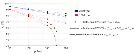
Figure 22.
Comparison of the results in terms of the volumetric efficiency from three sets of simulations, considering the case of unit 3 of Table 3.
In Figure 19, the deviation of the isothermal model from the thermal model and the experiments started to occur at low efficiency conditions. To further explore this effect, simulations were conducted at higher pressures. From Figure 22, at low efficiency conditions (), the isothermal models (even the one with mean temperatures) predict significantly higher volumetric efficiency compared to the thermal model. This is expected since, at low efficiency conditions, there is a significant amount of power loss in the EGM. This power loss is converted into heat raising the temperature of the fluid. As a consequence, the viscosity of the fluid is reduced, increasing the leakage flows and hence further lowering the volumetric efficiency. This phenomenon is not considered in the isothermal model justifying the observed difference in the volumetric efficiency.
At 1000 rpm, 200 bar, the thermal-HYGESim model predicts zero volumetric efficiency (the leakage flow exceeds the delivery flow) indicating that the EGM is inoperable at that operating condition. However, the isothermal model (set 1) predicts .
Thus, the thermal-HYGESim model is critical in the accurate efficiency prediction of the EGMs that exhibit low efficiency (also shown via experimental comparison in Section 3.4). This model is especially crucial in the prediction of the operability of the EGMs at extreme operating conditions (e.g., high temperatures and high pressures) and EGMs with worn out internal components (increasing the clearances, and thus the leakage flows).
4. Conclusions
This paper presents a thermal model for simulating the operation of external gear machines (EGMs). The model is based on the lumped parameter approach where the fluid domain is divided into several control volumes (CVs). The paper first describes the numerical approach for the evaluation of pressure and temperature in these CVs and mass and enthalpy flows across the CVs. Further, the approaches for the evaluation of friction at key interfaces and the power losses associated with them are described. The model developed in this work is integrated with the EGM simulation tool HYGESim developed by authors in the past.
The results of the proposed thermal model are then discussed for the case of gear pumps. The model reveals how during the pump operation, the temperature of the fluid increases as it is carried from the inlet to the outlet side. Further, the temperature of all the CVs in the EGM is observed to be higher than the temperature of the fluid at the inlet port. Among all the CVs, the drain volume has the highest temperature.
To validate the model, multiple experiments were conducted on six units of the reference EGM with different geometry of the gears, with respect to conicity and eccentricity. The comparison between the modelling predictions and the measured data shows a good agreement in terms of the outlet temperature and the volumetric efficiency, indicating the validity of the model developed in this work.
From the model results, it is shown that, while the traditional isothermal model can be suitable for modelling moderately efficient EGMs, the thermal model is indispensable for accurately modelling the performance of EGMs with poor efficiency and predicting the operability of EGMs at extreme operating conditions. Moreover, the thermal model is also crucial for the accurate prediction of the outlet temperature, which is valuable in the design and analysis of the hydraulic systems connected downstream of the EGMs.
Author Contributions
Conceptualization, R.R. and A.V.; methodology, R.R. and A.V.; software, R.R. and A.V.; validation, R.R.; formal analysis, R.R.; investigation, R.R. and M.A.M.; resources, A.V.; data curation, R.R.; writing—original draft preparation, R.R.; writing—review and editing, R.R. and A.V.; visualization, R.R.; supervision, A.V.; project administration, A.V. All authors have read and agreed to the published version of the manuscript.
Funding
This research received no external funding.
Conflicts of Interest
The authors declare no conflict of interest.
Nomenclature
| Width of the leakage gap | |
| Orifice flow coefficient | |
| Specific heat of the fluid | |
| Unit vector | |
| Force | |
| Enthalpy flow rate | |
| Specific enthalpy of the fluid | |
| Leakage gap height | |
| Isothermal bulk modulus | |
| Length of the leakage gap | |
| Distance of the line of action of forces from the gear center | |
| Moment | |
| Mass | |
| Mass flow rate | |
| Shaft speed | |
| Number of ports in a generic CV | |
| Pressure | |
| Heat flow rate | |
| Heat flux | |
| Radius | |
| Temperature | |
| Time | |
| Internal energy | |
| Volume | |
| Relative velocity of the two surfaces at the leakage interface | |
| Rate of work done | |
| Cartesian directions | |
| Subscripts | |
| Friction | |
| Drain | |
| Gear | |
| Iterators | |
| Inlet | |
| Outlet | |
| Meshing | |
| Pressure | |
| Root | |
| Tip | |
| Lateral | |
| Greek letters | |
| Isobaric thermal expansion coefficient | |
| Conicity error | |
| Concentricity error | |
| Volumetric efficiency | |
| Angular position | |
| Viscosity of the fluid | |
| Density of the fluid | |
| Shear stress | |
| Area | |
| Rotational velocity of the gear | |
| Abbreviations | |
| CV | Control Volume |
| EGM | External Gear Machine |
| EHL | Elastohydrodynamic lubrication |
| TSV | Tooth Space Volume |
Appendix A. Derivation of Pressure Build up Equation
For the generic CV in Figure 5, the conservation of mass equation can be written as:
Applying chain rule:
Now, the total derivative of density can be written as:
For the working fluid, isothermal bulk modulus is defined as:
and the isobaric thermal expansion coefficient is defined as:
Thus, Equation (A5) becomes
Substituting from Equation (A3) in (A8),
Appendix B. Derivation of Temperature Rise Equation
For the generic CV in Figure 5, the conservation of energy equation can be written as:
where is the internal energy of the CV which can be expressed in terms of the specific enthalpy, , as:
The boundary work done by the CV is . Thus,
Upon simplification,
Now, the specific enthalpy can be expressed as a function of temperature and pressure as
Detailed derivation of this relationship can be found in [21].
Eliminating from Equations (B4) and (B5), the governing equation for the temperature in a CV is obtained:
References
- Ivantysyn, J.; Ivantysynova, M. Hydrostatic Pumps and Motors: Principles, Design, Performance, Modelling, Analysis, Control, and Testing; Akademia Books International: New Delhi, India, 2001; ISBN 8185522162. [Google Scholar]
- Dhar, S.; Vacca, A. A fluid structure interaction—EHD model of the lubricating gaps in external gear machines: Formulation and validation. Tribology Int. 2013, 62, 78–90. [Google Scholar] [CrossRef]
- Bonacini, C. Sulla portata delle pompe ad ingranaggi. In Proceedings of the L’Ingegnere, Anno, Milan, Italy, January 1961. [Google Scholar]
- Manring, N.D.; Kasaragadda, S.B. The theoretical flow ripple of an external gear pump. J. Dyn. Syst. Meas. Control 2003, 125, 396. [Google Scholar] [CrossRef]
- Manco, S.; Nervegna, N. Simulation of an external gear pump and experimental verification. Proc. JFPS Int. Symp. Fluid Power 1989, 1989, 147–160. [Google Scholar] [CrossRef]
- Eaton, M.; Keogh, P.S.; Edge, K.A. The Modelling, prediction, and experimental evaluation of gear pump meshing pressures with particular reference to aero-engine fuel pumps. Proc. Inst. Mech. Eng. 2006, 220, 365–379. [Google Scholar] [CrossRef]
- Zardin, B.; Paltrinieri, F.; Borghi, M.; Milani, M. About the prediction of pressure variation in the inter-teeth volumes of external gear pumps. In Proceedings of the 3rd FPNI-PhD Symposium on Fluid Power, Barcellona, Spain, 30 June–2 July 2004. [Google Scholar]
- Zardin, B.; Borghi, M. Modeling and simulation of external gear pumps and motors. In Proceedings of the 5th FPNI—PhD Symposium on Fluid Power, Krakow, Poland, 1 January 2008. [Google Scholar]
- Falfari, S.; Pelloni, P. Setup of a 1D model for simulating dynamic behaviour of external gear pumps. In Proceedings of the SAE 2007 Commercial Vehicle Engineering Congress & Exhibition, Rosemont, IL, USA, 30 October 2007. [Google Scholar]
- Mucchi, E.; Dalpiaz, G.; Fernandez Del Rincon, A. Elastodynamic analysis of a gear pump. Part I: Pressure distribution and gear eccentricity. Mech. Syst. Signal Process. 2010, 24, 2160–2179. [Google Scholar] [CrossRef]
- Vacca, A.; Guidetti, M. Modelling and experimental validation of external spur gear machines for fluid power applications. Simul. Model. Pract. Theory 2011, 19, 2007–2031. [Google Scholar] [CrossRef]
- Devendran, R.S.; Vacca, A. Optimal design of gear pumps for exhaust gas aftertreatment applications. Simul. Model. Pract. Theory 2013, 38, 1–19. [Google Scholar] [CrossRef]
- Zhao, X.; Vacca, A. Formulation and optimization of involute spur gear in external gear pump. Mech. Mach. Theory 2017, 117, 114–132. [Google Scholar] [CrossRef]
- Strasser, W. CFD investigation of gear pump mixing using deforming/agglomerating mesh. J. Fluids Eng. 2007, 129, 476. [Google Scholar] [CrossRef]
- Castilla, R.; Gamez-Montero, P.J.; Del Campo, D.; Raush, G.; Garcia-Vilchez, M.; Codina, E. Three-dimensional numerical simulation of an external gear pump with decompression slot and meshing contact point. J. Fluids Eng. 2015, 137, 041105. [Google Scholar] [CrossRef]
- Qi, F.; Dhar, S.; Nichani, V.H.; Srinivasan, C.; Wang, D.M.; Yang, L.; Bing, Z.; Yang, J.J. A CFD study of an electronic hydraulic power steering helical external gear pump: Model development, validation and application. SAE Int. J. Passeng. Cars Mech. Syst. 2016, 9, 346–352. [Google Scholar] [CrossRef]
- Manco, S.; Nervegna, N. Experimental Investigation on the Efficiency of an external gear pump by the thermodynamic method. In Proceedings of the 2nd Bath International Fluid Power Workshop on Components and Systems, Bath, UK, 21–22 September 1989; pp. 259–273. [Google Scholar]
- Dalla Lana, E.; De Negri, V.J. A new evaluation method for hydraulic gear pump efficiency through temperature measurements. SAE Tech. Pap. 2006, 1, 3503. [Google Scholar] [CrossRef]
- Casoli, P.; Campanini, F.; Bedotti, A.; Pastori, M.; Lettini, A. Overall efficiency evaluation of a hydraulic pump with external drainage through temperature measurements. J. Dyn. Syst. Meas. Control 2018, 140, 081005. [Google Scholar] [CrossRef]
- Zecchi, M.; Mehdizadeh, A.; Ivantysynova, M. A novel approach to predict the steady state temperature in ports and case of swash plate type axial piston machines. In Proceedings of the Proceedings from the 13th Scandinavian International Conference on Fluid Power, Linköping, Sweden, 3–5 June 2013; Volume 92, pp. 177–187. [Google Scholar]
- Shang, L.; Ivantysynova, M. Port and case flow temperature prediction for axial piston machines. Int. J. Fluid Power 2015, 16, 35–51. [Google Scholar] [CrossRef]
- Dhar, S.; Vacca, A.; Lettlnl, A. A novel fluid-structure-thermal interaction model for the analysis of the lateral lubricating gap flow in external gear machines. In Proceedings of the ASME/BATH 2013 Symposium on Fluid Power and Motion Control, FPMC 2013, New York, NY, USA, 6–9 October 2013. [Google Scholar]
- Dhar, S.; Vacca, A. A novel FSI-thermal coupled TEHD model and experimental validation through indirect film thickness measurements for the lubricating interface in external gear machines. Tribol. Int. 2015, 82, 162–175. [Google Scholar] [CrossRef]
- Simcenter Amesim Help, version 2019.1; Siemens AG: Munich, Germany, 2019.
- Concentric GC series hydraulic pumps. In Concentric Hydraulics Catalog; Concentric Hydraulics: Rockford, IL, USA, 2018.
- Merritt, H.E. Hydraulic Control Systems; John Wiley & Sons, Inc.: New York, NY, USA, 1967. [Google Scholar]
- Jacobson, B.O.; Hamrock, B.J. Non-Newtonian fluid model incorporated into elastohydrodynamio lubrication of rectangular contacts. J. Tribol. 1984, 106, 275–281. [Google Scholar] [CrossRef]
- Trippett, R.J. Ball and needle bearing friction correlations under radial load conditions. SAE Tech. Pap. 1985, 94, 646–653. [Google Scholar] [CrossRef]
- Booker, J.F. Dynamically loaded journal bearings: Mobility method of solution. J. Basic Eng. 1965, 87, 537. [Google Scholar] [CrossRef]
- Zhao, X.; Vacca, A. Numerical analysis of theoretical flow in external gear machines. Mech. Mach. Theory 2017, 108, 41–56. [Google Scholar] [CrossRef]
- Pellegri, M.; Manne, V.H.B.; Vacca, A. A simulation model of Gerotor pumps considering fluid–structure interaction effects: Formulation and validation. Mech. Syst. Signal Process. 2020, 140, 106720. [Google Scholar] [CrossRef]
- Monika, B.K.; Magdalena, M.M.; Pawel, M.R. ANSYS academic research mechanical, release 19.1. In Recent Trends in Environmental Hydraulics: 38th International School of Hydraulics; Springer: Berlin/Heidelberg, Germany, 2018. [Google Scholar]
- Rituraj, F.; Vacca, A.; Morselli, M.A. Modeling of manufacturing errors in external gear machines and experimental validation. Mech. Mach. Theory 2019, 140, 457–478. [Google Scholar] [CrossRef]


© 2020 by the authors. Licensee MDPI, Basel, Switzerland. This article is an open access article distributed under the terms and conditions of the Creative Commons Attribution (CC BY) license (http://creativecommons.org/licenses/by/4.0/).