Abstract
The high penetration of renewable energy sources, combined with a limited possibility to expand the transmission infrastructure, stretches the system stability in the case of faults. For this reason, operators are calling for additional control flexibility in the grid. In this paper, we propose the deployment of switchable reactors and capacitors distributed on the grid as a control resource for securing operations during severe contingencies and avoiding potential blackouts. According to the operating principles, the line reactance varies by switching on or off a certain number of distributed series reactors and capacitors and, therefore, the stabilizing control rule is based on a stepwise time-discrete control action. A control strategy, based on dynamic optimization, is proposed and tested on a realistic-sized transmission system.
1. Introduction
Flexible AC transmission systems (FACTS) have always been considered as a simpler and cheaper alternative to High Voltage Direct Current (HVDC) systems to increase grid controllability [1]. FACTS series compensating devices have been traditionally studied for improving static operative conditions, such as in optimal power flow applications [2]. For example, thyristor controlled series compensators (TCSC) can influence power flows by varying the transmission lines equivalent impedance. TCSC have been considered in transmission expansion planning [3] and in increasing the integration of wind power plants [4], due to the improved power flow capability. However, the application of such equipment is not limited to steady-state applications; it can be extended to transient stability [5]. The dynamic series control of transmission lines relies on the idea that the equivalent reactance of transmission lines can be controlled along transients to damp system oscillations, avoiding power system instability after large perturbations [6], or damping resonances, which can endanger the system stability [7].
In their previous work, the authors showed that TCSCs ensure effective performances in controlling power system transients following severe contingencies [8]. In particular, TCSCs have been assumed as actuators of corrective control actions that follow a specific occurrence (i.e., angle instability following a severe fault) of a set of pre-postulated unstable system contingencies in an on-line Dynamic Security Assessment (DSA) framework. TCSCs represent a good option for angle stability control, because of their high reliability and their ability to provide a continuous control of the equivalent series reactance [9]. As an alternative to continuous control actions, in [10], a dynamic line switching is proposed as series control action for avoiding transient instability. Following the solution of a pre-calculated optimal problem, selected lines are switched off/on during the transients, in order to redistribute the power flow, and damp the system oscillations.
Although TCSCs, and more in general FACTS technology, constitute a well known and technically proven solution for improving power system static and dynamic behavior, a widespread deployment of such devices is not foreseeable due to their high capital and operating costs. It is also recognized that TCSCs might be too expensive to be adopted in power systems if their functions are only oriented to power system security. Possible applications are found in network reinforcement planning under large wind power plants integration [11] and high power demand scenarios [12].
On the other side, alternative devices in the series-connected FACTS family can offer comparable control capabilities (both inductive and reactive series compensation) at smaller costs. Thyristor switched series compensators (TSSCs) and thyristor switched series reactors (TSSR) [13], for example, are simpler (and less expensive) FACTS series devices that can provide a stepwise control of the line reactance, by switching on/off, respectively, series-connected capacitors and reactors. Possible applications of such devices are for increasing the grid stability, solving the transmission lines congestion, or improving the grid power quality [14] Although rarely coupled together, hybrid combination of these two devices can be found in [15,16], where a hybrid flow controller (HFC) design has been proposed to mimic unified power flow controller (UPFC) functions with a simpler architecture. Although HFC architecture is aimed at achieving control of both series and shunt variables, the design of its series section suggests that a coupling of TSSRs and TSSCs provides a stepwise control of series line impedance without the need of inserting a series voltage (as in more complex FACTS, such as static synchronous series compensator (SSSC) and, of course, UPFC). A novel alternative approach to exploit series parameters for transient stability purpose is proposed in [17,18,19], under the names of distributed-FACTS (D-FACTS), distributed series impedance (DSI), and distributed series reactor (DSR) devices, respectively. These components are characterized by lower costs and consist of distributed series reactors and capacitors distributed in the transmission lines, which can provide both inductive and capacitive series compensation. They are characterized by an innovative design that permits reducing investment costs. Indeed, D-FACTS can be installed directly on power lines (clamp-on) absorbing the energy necessary to supply power electronics and communication components through inductive coupling. The series coupling of D-FACTS is obtained with a single-turn transformer that uses the transmission line itself as secondary winding and constitutes the main power conversion section of a D-FACTS [20]. This architecture allows huge savings in terms of voltage insulation and on-site installation. Recent applications of D-FACTS have been studied for voltage control and stabilization of microgrids [21] and distribution systems [22].
This paper explores the possibility of controlling transient stability of the bulk power system, enabling a time-variant control of transmission line reactance by means of D-FACTS. According to the operating principles of TSSR, TSSC, and DSI, the line reactance is changed by switching on or off a certain number of distributed series reactors and capacitors, and, therefore, the stabilizing control rule is based on a stepwise time-discrete control function. The approach proposed for estimating the control action is based on the dynamic programming techniques introduced in [23]. With respect to the previous works of the authors [8], this paper studies the discrete nature of the D-FACTS. On the opposite of series compensators such as TCSCs that can vary their equivalent impedance in continuous way, D-FACTS can act only in discrete steps. This work takes into account the discrete nature of D-FACTS, developing a mathematical approach for discrete impedance variation, that differs from the continuous one proposed in [8,23]. In particular, a parameter variation analysis of the different control time windows and control variable quantization was performed to validate the proposed approach.
This paper is structured as follows. In Section 2, the technology and basic operation principle of D-FACTS is introduced. The optimization algorithm is developed in Section 3, depicting the objective functions and the system constraints. Test results representing the Italian power system and an equivalent of the ENTSO-E network in a transient stability software in are presented in Section 4, including the parameter variation analysis for different control time windows and variable quantization. Finally, the conclusions are drawn in Section 5.
2. Series Compensation and D-FACTS Basic Operation Principle
The TSSC (or TSSR) basic operation principle can be described as a series of capacitors (or reactors) shunted by a thyristor-switched bypass branch. By controlling the thyristors, it is possible to modify the apparent line series reactance with the series insertion of a certain number of capacitors (or reactors). TSSCs and TSSRs, whose basic schemes are given, respectively, in Figure 1 and Figure 2, are relatively simple and reliable devices, if compared with more complex solutions, such as UPFC. They are characterized by a very mature and well-tested architecture that can be placed in electrical substations in order to achieve series capacitive or inductive compensation of a power line. Although rarely coupled together, a combination of TSSR and TSSC has been proposed in the literature to provide a wide range of reactance control in transmission lines [15,16].
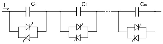
Figure 1.
Thyristor switched series compensators (TSSC) basic scheme.
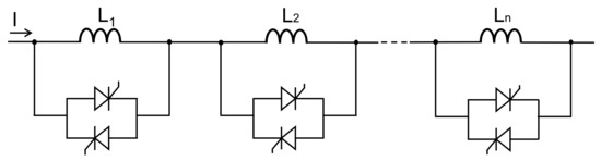
Figure 2.
Thyristor switched series reactors (TSSR) basic scheme.
D-FACTSs [17,18] follow the same operating principles as other traditional FACTS. Differently from TSSR and TSSC, they consist of several power electronic-controlled devices distributed along the transmission lines and not concentrated in the substations. Each component is supposed to be directly installed on line conductors. They are light enough to be suspended mechanically on transmission lines and can be easily installed on existing lines thanks to their clamp-on design. The energy necessary to the supply the control system of each component is taken directly from the conductors thanks to an inductive coupling.
As the main advantages of D-FACTS, being suspended on the line, the devices do not require any phase-ground insulation and can, therefore, be applied to any transmission voltage level. This condition allows saving a great amount of money (and weight) with respect to other lumped FACTS devices that, being installed on the ground, do actually require suitable voltage insulation.
D-FACTS show many other possible advantages if compared to traditional series-connected FACTS devices. The low Volt–ampere ratings of each module allows employing ordinary power electronics components (e.g., 1.2/1.7/3.3. kV IGBT) that are used in the large-scale manufacturing of wind turbine converters [24]. This means that each component can be produced at an extremely low cost, especially if compared to big FACTS installations that require high-voltage, high-power semiconductors and passive elements (e.g., capacitors and inductors). Moreover, the design with a large number of modules leads in higher system reliability, because global system operation are not affected by the failure of few devices. The clamp-on configuration also permits faster maintenance operations.
It should also be remarked that modular configurations of D-FACTSs are compatible with gradual deployment strategies, allowing the system operator to distribute its economic investments more suitably across time. For example, priority can be given to stressed corridors, where few D-FACTS can be installed firstly on those lines that more often experience congestions or other security problems. Further components can be installed instead at a later time, whenever other security issues should arise or new economic resources be available.
Series coupling D-FACTS, such as Distributed Series Impedance (DSI) devices and with a basic design, as sketched in Figure 3, allow combining the capabilities of both TSSC and TSSR schemes and achieving a stepwise control of series reactance, operating in both capacitive active and reactive ranges. Each module, as demonstrated in [18], can be controlled in order to increase or decrease the overall series impedance of the line. A single turn transformer is employed to achieve the series compensation, exploiting the line conductor as a transformer winding.
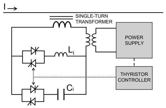
Figure 3.
Basic scheme of a series coupling D-FACTS device.
Even though each device is able to achieve a small compensation, the coordinated control of a large number of modules enables a wide range of control. Therefore, DSIs can mimic the control capability that can be obtained though the coupling of large TSSC and TSSR installations. Figure 4 shows how line reactance can vary with the switching on/off of the distributed devices.
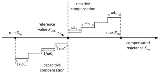
Figure 4.
Stepwise capacitive and inductive series compensation of line reactance.
The control system of all D-FACTS installed on a single transmission line can be based on signals that are received via radio or wireless communication systems. Clearly, both centralized and local control architectures are possible. The control signals can be transmitted from the control center, or thyristors can follow pre-programmed schemes that are based on simple current threshold or more complex feedback control loops.
Although series coupling FACTS and D-FACTS are mostly conceived for steady state optimization of power flows and for static security enhancement, it is envisioned that series compensation might be adopted on critical interfaces for controlling power system dynamic behavior. In this vision, any series-connected device could be exploited for stretching or shrinking dynamically transmission lines, in order to ensure proper transient behavior.
In this paper, a methodology for evaluating an optimal control rule to be applied to a cluster of switchable capacities or reactance in order to stabilize the transient following a pre-postulated severe contingency is proposed. This means that such devices might be employed as actuators of corrective control actions to be applied during the transient in order to preserve the integrity of the system. The proposed approach is general enough to be applied to both lumped (TSSC/TSSR) and distributed (DSI) configurations since a similar control of series equivalent reactance, which can be represented as shown in Figure 4, is provided. Clearly, the employment of distributed controlled devices would require wider communication systems, since the control signals, sent by the control center to the sending bus or the receiving bus of the transmission lines equipped with D-FACTS, will have to be communicated to the modules distributed along the line with any wireless technology (for example, radio signals).
The control law to be implemented is based on the switching of discrete elements and is therefore based on stepwise functions. Moreover, to take into account the time necessary to complete the variation of capacitive or inductive reactance (i.e., the time necessary to complete the electrical transients within the internal circuits of the devices), it is supposed that the controlled devices can change their status only once within a selected time window. This window must be large enough to include the time necessary to communicate the next window’s control action to the cluster of controlled devices. An assessment of the impact of the window’s width on the efficacy of the control action is shown in the test results. Clearly, communication delays, which can be in the order of hundreds of milliseconds, have a preponderant weight with respect to the electrical transients that can be considered completed within half a cycle (10 ms).
3. Optimization Algorithm
The mathematical formulation can be partly derived from the one proposed in [8], where an approach to control dynamically degree of compensation of TCSCs is described. As in [8], the proposed methodology is based on the approach developed in [23]. A dynamic optimization problem is converted into nonlinear programming, discretizing the differential algebraic equations (DAEs) that represent the system dynamic behavior.
In [8], two algorithms are proposed, one aimed at the definition of an ideal time-varying control rule (optimal solution) and another that evaluates a suboptimal solution, consisting on time stepwise changes of the TCSC’s reference signal. In this paper, we assume to apply subsequent stepwise changes along the transient, mimicking the stepwise characteristic of D-FACTS described in Figure 4. In the proposed optimization algorithm, each step change is evaluated for a specific control time window. The size of this time window must take into account control delays due to communication bottlenecks or the time necessary for the synchronization of all distributed control actions.
3.1. Mathematical Formulation
3.1.1. Equality Constraints
Assuming to work in electromechanical transient time-range, a specific set of nonlinear DAEs can be employed to represent the transient behavior of a power system with nB buses and nG generators:
where x represents the p-dimensional state vector, V denotes the vector of 2nB nodal voltages, and u is the nL-dimensional vector of control signals.
Adopting a general implicit integration rule, the DAEs set can be discretized at each generic ith time step:
with
where nT is the total number of time steps relative to the control time window and k are the time steps of the adopted implicit discretization rule (k ≤ i). In this paper a trapezoidal rule is adopted (k equals 1).
Synthetically, Equation (3) can be written as
where the discretized differential algebraical equations , the state variables and nodal voltages , and control variables are formulated as follows:
The DAEs discretized equations can be considered the equality constraint of the overall nonlinear programming problem just as the differential equations are the equality constraint in optimal control problems.
3.1.2. Control Variables
The set of control variables describes the level of compensation of each transmission line where the D-FACTS are installed. In each control time window, the control variable is constant and can be defined as:
where w is the wth control time window and and are, respectively, the value of the equivalent compensated series admittance and the uncompensated series admittance for the jth controlled line. Assuming that the controlled lines are nL and each time window is composed by nTW time steps, and
the time-varying control variable vector at the generic ith time step is:
In [16], it is shown how the deployment of a single D-FACTS module at every mile of a transmission line can achieve a control capability of about 2% of the overall line reactance. On the basis of such information, it is reasonable to assume that the line reactance can vary in the range 0.9–1.1 p.u. corresponding to an approximate value of five devices for each mile. This range considers also the need for avoiding sub-synchronous resonances, created by overcompensation of the line [25]. According to this assumption, the control variables are constrained in the capacitive and inductive range through hard inequality constraints:
Please note that can only assume discrete values due to the discrete nature of the switching actions of the controllers. In the algorithm, the control variables are assumed to vary continuously in the interval 0.9–1.1 p.u., whereas the discrete values, at the end of the optimization routine, are adjusted to meet the closest discrete set point. However, since the D-FACTS devices are expected to be numerous, the approximation due to the discretized control action do not introduce relevant changes in the effects of the overall control law, as shown in the test results.
3.1.3. Objective Function
The goal of this work is to prevent angle-instability-related cases and thus to enhance transient stability. Consequently, an objective function is formulated to minimize the transient kinetic energy (TKE) and defined as:
with
where is the computed TKE with respect to the system centre of inertia (COI) at any ith time step, is the rotor speed of the mth generator at the ith time step, represents the COI speed at the ith time step, and Mm is the mth generator rotor inertia.
3.2. Optimization Algorithm
Once the objective cost function is defined, the optimization problem can be formulated as:
subject to the equality constraints in Equation (6) and to the hard inequality constraints in Equation (13).
This problem is formulated as a constrained minimization, which can suitably be changed into an unconstrained problem by defining a Lagrange function:
where γ is the Lagrangian multiplier vector. Summarizing, an optimal solution can be achieved by solving the following set of equations:
For a better understanding of the workflow of the algorithm, the flowchart in Figure 5 is shown. Equations (18)–(20) are solved through a generalized reduced gradient method (GRG), which yields a simple code structure, where ordinary power flow and transient stability routines can be employed.
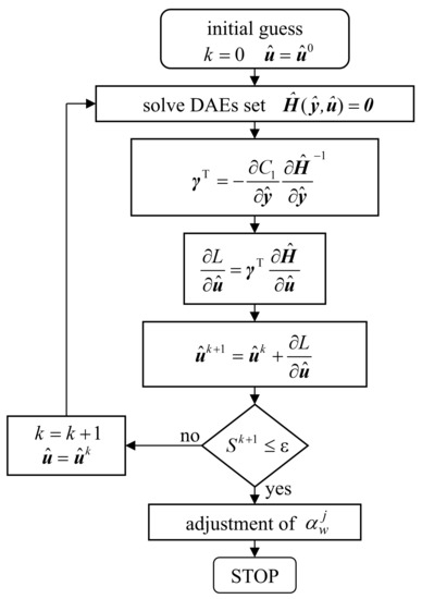
Figure 5.
Flowchart of the solving algorithm.
To achieve an optimal solution, a stopping criterion is defined. If the maximum mismatch between two subsequent iterations is lower than a predefined tolerance value ε, the algorithm stops and gives the solution in output. The adopted stopping criterion is:
with
where is the control variable at the generic wth control time window for the jth controlled line at the iteration kth of the algorithm. The tolerance in Equation (21) was assumed equal to 0.01 p.u. As shown in Figure 5, after convergence, the algorithm adjusts each control variables to meet the closest discrete set point available for the jth controller.
4. Test Results
To validate the proposed D-FACTS approach, a realistic-sized model of the Italian power grid and a part of the interconnected ENTSO-E network was simulated. The test network is characterized by 1333 buses, 1762 lines, 769 transformers, and 294 generators.
As placement assumption, it was supposed that several D-FACTS devices are installed on the following 380 kV transmission lines (marked with colors in Figure 6): Villanova-Montalto, Villanova-Larino, and Latina-Garigliano. Please note that the figure is purely explicative and that the arrows point to generic segments of the controlled transmission lines and not to the specific location of the devices.
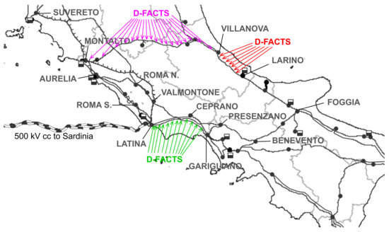
Figure 6.
Portion of the Italian 380 kV transmission grid (Central-Southern Italy).
4.1. Base Case
In the simulations, a base case with a 37.5% uniformly distributed overload with respect to the original operative state was assumed, targeting the reproduction of the actual Italian power system conditions during the morning peak of a working day. Under these significantly overloaded conditions, the power system shows unstable transient behavior if a three-phase fault hits the 380 kV transmission line Aurelia-Roma and it is cleared after 100 ms. Note that this overloaded condition is not representative of an actual operating system state. For testing, the grid is far from the normal operating conditions.
As can be noted in Figure 7, collecting the angle trajectory of all 294 generators, calculated with respect to the system COI, several generators lose synchronism after the first swing. In the figure, it is clear how a group of generators, mostly located in Sicily, separates from the rest of the Italian system. The voltage trajectories, represented in Figure 8 for each bus, shows also the typical behavior of angle instability with several nodes reaching a voltage magnitude close to zero. Please note that, for the sake of clarity, all voltage magnitudes are represented in p.u., with respect to the pre-fault voltage.
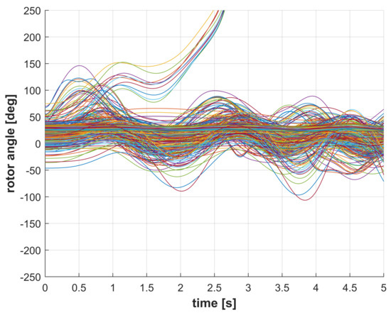
Figure 7.
Rotor angles in the uncontrolled case.
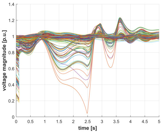
Figure 8.
Voltage magnitudes in the uncontrolled case.
The optimization algorithm was then applied to this specific contingency, considering a control window with a 200 ms step size. This means that the D-FACTSs vary the equivalent impedance every 200 ms and not in a continuous way. As outcome from the algorithm convergence, the control actions shown in Figure 9 were obtained. In the figure, it is clear that the algorithm tries to increase the equivalent admittance of the lines, in order to reduce the electrical distances among generators, and thus to enhance the system stability.
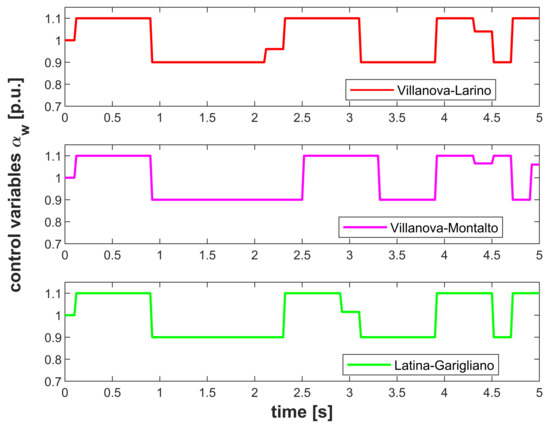
Figure 9.
Control actions for the three clusters of D-FACTS.
The implementation of these control actions on the D-FACTS permits stabilizing the system, obtaining a stable angle behavior, as shown in Figure 10, where the previously unstable generators gain stability after the first swing. This is more clearly shown in Figure 11 that compares the rotor angle trajectory of one of the unstable generators in Sicily in the controlled and uncontrolled case. Figure 12 shows the voltage behavior of all nodes. Due to the severity of the fault, as in the previous case, some voltages drop consistently. As shown in Figure 13, the major voltage variations are experienced on the corridor interconnecting Sicily with the rest of the Italian peninsula. The group of Sicilian generators oscillates with respect to the rest of the Italian generators, causing the voltage to drop on the interconnection. In the controlled case, voltage excursions are still consistent but are rapidly damped out. The overall voltage behavior can be considered acceptable.
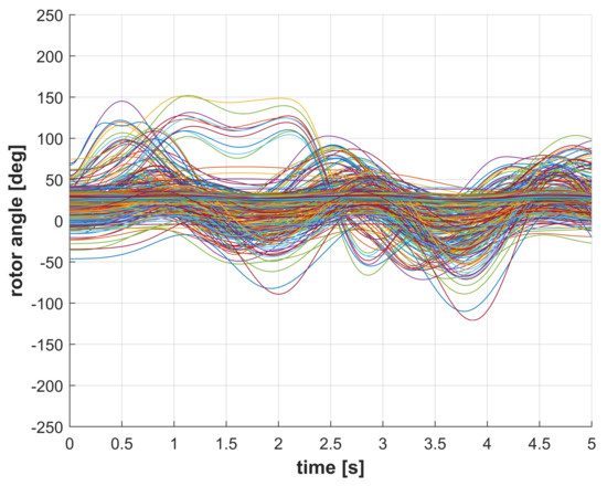
Figure 10.
Rotor angles with D-FACTS control.
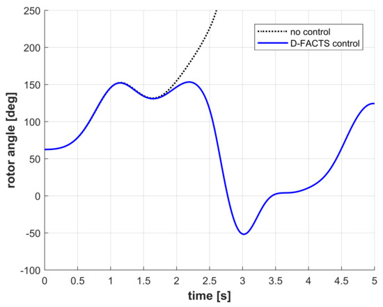
Figure 11.
Rotor angle trajectory of the generator in Termini Imerese (Sicily).
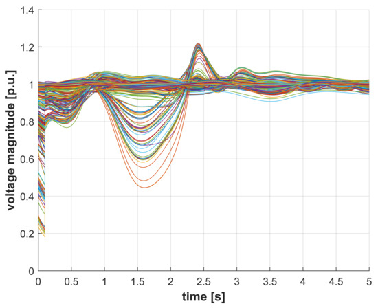
Figure 12.
Voltage magnitude with D-FACTS control.
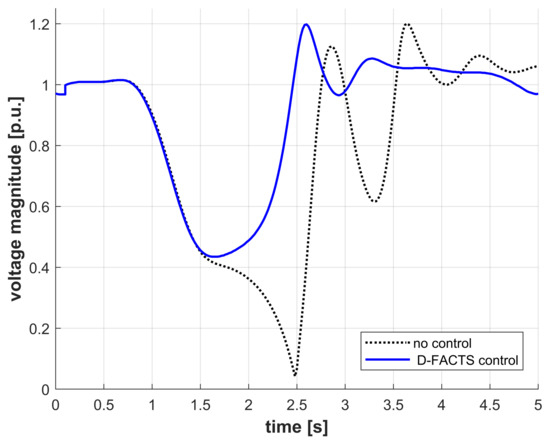
Figure 13.
Voltage magnitude trajectory at the 400-kV Rizziconi busbar (Calabria).
4.2. Impact of the Control Time Window
Further tests were devoted to assess the dependence of the proposed control strategy performance with respect to the size of the control time window. These tests were carried out considering the same unstable base case presented in the previous section and applying the control actions on time windows with growing sizes: 200 ms (the case considered previously), 500 ms, 1 s, and 5 s. Since the simulation ran for 5 s, the case with the largest window (5 s) corresponded to the condition where only a single step variation of the line reactance was applied. By reducing the control time window, it is possible to get progressively closer to the ideal optimal control solution where the control law varies at each time step. For several reasons, such as the presence of communication delays, the increase of such delays in relation to an increase of the data to be transmitted to the actuators, and the necessity to synchronize the time-varying response of several devices, this ideal control solution is considered impractical. Figure 14 shows the impact of the different control windows on the Villanova-Montalto line.
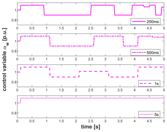
Figure 14.
Control action applied to the D-FACTS in Villanova-Montalto with different control time windows.
In all four simulated cases, the system response is stable, proving the robustness of the approach with regard to the time window size. However, in general, it is possible to observe that the power system dynamic response deteriorates while the size of the control time window increases, since the solution gets progressively more distant from the ideal one, which would assume a continuous variation of the control signal at each instant. The rotor angle and voltage trajectories obtained with a single-shot step-change 5 s window are shown in Figure 15 and Figure 16. The time response does not differ very much from the previous case, obtained with a 200 ms time window (Figure 10 and Figure 12), although it can be observed that the voltage dynamics are damped out a little more slowly.
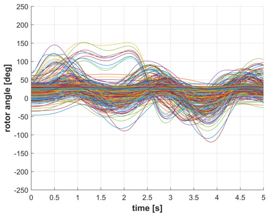
Figure 15.
Rotor angles with a “single-shot” 5 s window D-FACTS control.
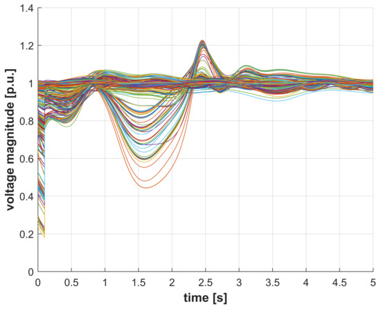
Figure 16.
Voltage magnitude with a “single-shot” 5 s window D-FACTS control.
Table 1 permits to associate some performance indices to the transient responses obtained with different control laws. In particular, the time-varying optimal control law obtained with a 200 ms delay is compared to the “single-shot” solution which represents a suboptimal solution [8]. The comparison is made in terms of KTE, maximum instantaneous rotor speed difference, maximum instantaneous post-fault voltage difference, and possible interactions with distance protections. This last qualitative information, which can also be quantified and minimized in the optimization algorithm proposed in [26], can be very useful to verify the respect of what can be defined as practical stability. This means that, together with the classical properties and definitions of transient stability, in a stable system all trajectories should be contained in a dominion that ensures the respect of technical limits, avoiding possible undesired interaction with installed protection systems. The indices presented in the table show how the solution closest to the ideal optimal control is slightly better than the “single-shot” control action. Both responses are stable, although a degradation of the solution is noticeable from both angle and voltage trajectories. The very rapid crossing of the fourth zone in the “single-shot” case does not represent a big concern in terms of practical stability but is still and index of system stress.

Table 1.
Indicators of system dynamic performance.
4.3. Impact of the Control Variable Quantization
In the previous simulations, it was assumed that the control variables can assume any value in the interval 0.9–1.1 p.u. This is clearly a simplification because the level of compensation is determined by the discrete state of each D-FACTS installed on the jth transmission line. The last tests aimed at addressing this issue and evaluating the impact of the control variable granularity. The simulations considered a progressively decreasing number of available discrete steps. As an example, if a maximum of 20 steps can be used in the entire capacitive or inductive range (±0.1 p.u.), it follows that 20 D-FACTS are installed in the same line. As a consequence, the minimum discrete step-change of is ±0.005 p.u. To take into account their discrete nature, the control variables were first relaxed during the algorithm solution and then set to the closest possible discrete value during each simulation. The effects of the application of this approach on the final solution are shown in Figure 17 for the Villanova-Larino line, assuming different discretization steps. As can be observed the time-varying control laws, being characterized by a sort of “bang-bang” behavior, do not differ much from each other. The system response was equally stable in all simulated cases. As shown in Figure 18, the rotor angle trajectories of the most stressed generator in the three simulated cases are not distinguishable. The optimal control solution is barely degraded by the change of discretization step, suggesting that the approach is feasible also for lumped implementations of series compensation resources.
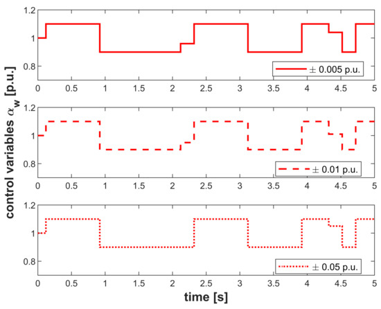
Figure 17.
Control laws for the Villanova-Larino line with different control variable discretization steps.
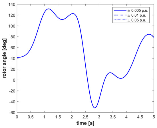
Figure 18.
Rotor angle of the Termini Imerese (Sicily) generator with different control variable discretization steps.
5. Conclusions
Higher stressed transmission systems call for more control flexibility if a higher integration of intermittent generation is planned. Of particular concern is the stability of such systems in overloaded conditions during faults. In this study, the potentials of the low cost technology provided by D-FACTS, distributed series compensator that vary the line impedance, was tested for controlling dynamic phenomena such as transient stability. The optimal control methodology was employed to provide a stepwise time-discrete control action, whose effectiveness was proven on a real transmission system through simulation. The test results show that unstable cases can regain stability if D-FACTS are applied, avoiding the lost of the weaker generator group in the simulated system. This work introduces two additional control parameter variations to validate the robustness of the algorithm under different control time windows and control granularity. The results show that the proposed control enhances the system stability, also in long control time window (e.g., 5 s, 25 times the base case) and low control action granularity (e.g., 0.05 p.u., ten times the base case).
Author Contributions
Conceptualization, S.B. and G.D.C.; methodology, M.L.S.; software, S.B. and M.L.S.; validation, S.B.; investigation, G.D.C.; resources, G.D.C.; data curation, M.L.S.; writing—original draft preparation, G.D.C.; writing—review and editing, S.B.; visualization, S.B.; and supervision, M.L.S. All authors have read and agreed to the published version of the manuscript.
Funding
G.D.C. gratefully acknowledges funding by the Ministry of Science, Research and the Arts of the State of Baden-Württemberg Nr. 33-7533.-30-10/67/1.
Conflicts of Interest
The authors declare no conflict of interest.
References
- Peng, F.Z. Flexible AC Transmission Systems (FACTS) and Resilient AC Distribution Systems (RACDS) in Smart Grid. Proc. IEEE 2017, 105, 2099–2115. [Google Scholar] [CrossRef]
- Povh, D. Use of HVDC and FACTS. Proc. IEEE 2000, 88, 235–245. [Google Scholar] [CrossRef]
- Esmaili, M.; Ghamsari-Yazdel, M.; Amjady, N.; Chung, C.Y.; Conejo, A.J. Transmission expansion planning including TCSCs and SFCLs: A MINLP approach. IEEE Trans. Power Syst. 2020. [Google Scholar] [CrossRef]
- Ziaee, O.; Choobineh, F. Optimal Location-Allocation of TCSCs and Transmission Switch Placement Under High Penetration of Wind Power. IEEE Trans. Power Syst. 2017, 32, 3006–3014. [Google Scholar] [CrossRef]
- Del Rosso, A.D.; Canizares, C.A.; Dona, V.M. A study of TCSC controller design for power system stability improvement. IEEE Trans. Power Syst. 2003, 18, 1487–1496. [Google Scholar] [CrossRef]
- Chakrabortty, A. Wide-Area Damping Control of Power Systems Using Dynamic Clustering and TCSC-Based Redesigns. IEEE Trans. Smart Grid 2012, 3, 1503–1514. [Google Scholar] [CrossRef]
- Kumar, A.; Shankar, G. Dynamic stability enhancement of TCSC-based tidal power generation using quasi-oppositional harmony search algorithm. IET Gener. Transm. Distrib. 2018, 12, 2288–2298. [Google Scholar] [CrossRef]
- Bruno, S.; De Carne, G.; La Scala, M. Transmission Grid Control Through TCSC Dynamic Series Compensation. IEEE Trans. Power Syst. 2016, 31, 3202–3211. [Google Scholar] [CrossRef]
- Jovcic, D.; Pillai, G.N. Analytical modeling of TCSC dynamics. IEEE Trans. Power Deliv. 2005, 20, 1097–1104. [Google Scholar] [CrossRef]
- Bruno, S.; D’Aloia, M.; De Carne, G.; La Scala, M. Controlling transient stability through line switching. In Proceedings of the 2012 3rd IEEE PES Innovative Smart Grid Technologies Europe (ISGT Europe), Berlin, Germany, 14–17 October 2012; pp. 1–7. [Google Scholar]
- Ugranli, F.; Karatepe, E. Coordinated TCSC Allocation and Network Reinforcements Planning with Wind Power. IEEE Trans. Sustain. Energy 2017, 8, 1694–1705. [Google Scholar] [CrossRef]
- Ziaee, O.; Alizadeh-Mousavi, O.; Choobineh, F.F. Co-Optimization of Transmission Expansion Planning and TCSC Placement Considering the Correlation Between Wind and Demand Scenarios. IEEE Trans. Power Syst. 2018, 33, 206–215. [Google Scholar] [CrossRef]
- Hingorani, N.; Gyugyi, L.; El-Hawary, M. Understanding FACTS: Concepts and Technology of Flexible AC Transmission Systems; IEEE: Piscataway, NJ, USA, 1999; pp. 1–432. [Google Scholar] [CrossRef]
- Ahmadi, A.; Gandoman, F.H.; Khaki, B.; Sharaf, A.M.; Pou, J. Comprehensive review of gate-controlled series capacitor and applications in electrical systems. IET Gener. Transm. Distrib. 2017, 11, 1085–1093. [Google Scholar] [CrossRef]
- Niaki, S.A.N.; Iravani, R.; Noroozian, M. Power-Flow Model and Steady-State Analysis of the Hybrid Flow Controller. IEEE Trans. Power Deliv. 2008, 23, 2330–2338. [Google Scholar] [CrossRef]
- Afzalian, A.A.; Nabavi Niaki, S.A.; Iravani, M.R.; Wonham, W.M. Discrete-Event Systems Supervisory Control for a Dynamic Flow Controller. IEEE Trans. Power Deliv. 2009, 24, 219–230. [Google Scholar] [CrossRef]
- Divan, D.; Johal, H. Distributed FACTS—A New Concept for Realizing Grid Power Flow Control. In Proceedings of the 2005 IEEE 36th Power Electronics Specialists Conference, Recife, Brazil, 16 June 2005; pp. 8–14. [Google Scholar]
- Johal, H.; Divan, D. Design Considerations for Series-Connected Distributed FACTS Converters. IEEE Trans. Ind. Appl. 2007, 43, 1609–1618. [Google Scholar] [CrossRef]
- Omran, S.; Broadwater, R.; Hambrick, J.; Dilek, M. DSR design fundamentals: Power flow control. In Proceedings of the 2014 IEEE PES General Meeting|Conference Exposition, National Harbor, MD, USA, 27–31 July 2014; pp. 1–5. [Google Scholar]
- He, Z.; Zhang, S.; Liu, Y.; Wu, F.; Sheng, G.; Jiang, X. Research on the Power Output Characteristics of a Coupling Transformer in D-FACTS. Energies 2019, 12, 4709. [Google Scholar] [CrossRef]
- Elmetwaly, A.H.; Eldesouky, A.A.; Sallam, A.A. An Adaptive D-FACTS for Power Quality Enhancement in an Isolated Microgrid. IEEE Access 2020, 8, 57923–57942. [Google Scholar] [CrossRef]
- Khanh, B.Q. A New Comparison of D-FACTS Performance on Global Voltage Sag Compensation in Distribution System. In Proceedings of the 2019 IEEE Asia Power and Energy Engineering Conference (APEEC), Chengdu, China, 29–31 March 2019; pp. 126–131. [Google Scholar]
- La Scala, M.; Trovato, M.; Antonelli, C. On-line dynamic preventive control: An algorithm for transient security dispatch. IEEE Trans. Power Syst. 1998, 13, 601–610. [Google Scholar] [CrossRef]
- Blaabjerg, F.; Liserre, M.; Ma, K. Power Electronics Converters for Wind Turbine Systems. IEEE Trans. Ind. Appl. 2012, 48, 708–719. [Google Scholar] [CrossRef]
- Pilotto, L.A.S.; Bianco, A.; Long, W.F.; Edris, A. Impact of TCSC control methodologies on subsynchronous oscillations. IEEE Trans. Power Deliv. 2003, 18, 243–252. [Google Scholar] [CrossRef]
- Bruno, S.; De Benedictis, M.; Delfanti, M.; La Scala, M. Preventing blackouts through reactive rescheduling under dynamical and protection system constraints. In Proceedings of the 2005 IEEE Russia Power Tech, St. Petersburg, Russia, 27–30 June 2005; pp. 1–8. [Google Scholar]
© 2020 by the authors. Licensee MDPI, Basel, Switzerland. This article is an open access article distributed under the terms and conditions of the Creative Commons Attribution (CC BY) license (http://creativecommons.org/licenses/by/4.0/).