Impact of Different Regulatory Structures on the Management of Energy Communities

Abstract

The following paper aims to prove the importance of embedding the regulatory framework when analyzing the distributed generation activity of an energy community. At present, most of the scientific literature has focused on distributed energy, and energy communities address the issue of regulatory frameworks qualitatively. In this paper, the most representative regulatory frameworks devoted to the promotion of energy communities were analyzed and synthesized, namely, feed-in tariffs, net metering, and the self-consumption scheme. As a result, an algebraic model able to represent the essence of the regulatory structures related to those remuneration mechanisms was obtained. Next, this model was embedded into a physical model, based on real data, previously created. The resulting Mixed Integer Linear Program (MILP) was used to identify the implications of these frameworks. The results demonstrate the impact of regulatory schemes on energy management and economic results of an energy community. Indeed, profitability changes drastically depending on which remuneration scheme is applied to an energy community.

1. Introduction

1.1. Context

The European Union (EU) is undergoing a change in the means in which electrical energy is produced, distributed, and sold for use in different appliances. This change is not only physical, that is, a change in the different structures and technologies to produce energy, but also philosophical: the goals of the EU include, among them, the installation of several facilities of distributed generation systems [1]. Opposed to the classical mass-production of electricity, where big power plants generate the required energy to supply hundreds of thousands of households and industries, the distributed generation scheme aims for an aggregation of, at most, a few hundred consumers, who will be capable of producing the energy that they require to satisfy their own needs.

The term “energy community” has been coined to define this type of aggregation [2]. An energy community makes use of the resources in their immediate environment to produce energy, mainly for self-consumption purposes. Its origin dates back to the anti-nuclear campaign and the oil crisis of the end of the 1970’s. Renewable energy started to be promoted [3] because of its several advantages over the conventional energy sources: decentralization, environmentally-friendliness, efficiency and durability. In Denmark, groups of people gathered their resources to buy wind turbines, establishing the first example of an energy community. The movement was fully recognized by the Danish government, establishing that country to be a pioneer of wind energy, and thus setting an example of how regulation can influence the renewable energy sector [4].

1.2. State of the Art—Justification of the Article and Main Contributions

A multitude of articles have been dedicated to the study of energy communities. First of all, it is worth emphasizing the informative articles, which introduce the concept and explain its tendencies. Koirala et al. [2] elaborate an exhaustive analysis of the concept of integrated systems in energy communities, presenting its different varieties and technologies, and comparing them, focusing on research applications, practical examples and viability in developing countries. Mancarella [5] develops a similar analysis, focusing on the coexistence of different elements of generation within the community and the advantages and disadvantages of considering them separately. Gui and MacGill [6] explore the different forms that clean energy communities can adopt and analyze the pathways that lead to their adoption. The authors mention the relevance of regulatory factors to improve the efficiency of energy communities. Hossain et al. [7] introduce a state-of-the-art study about microgrids and the different projects in which they have been included. At a national level, it is worth mentioning Rubio and Díaz’s article [8], which compares energy communities from Spain and Germany.

Soon, energy planning in energy communities will arise as a topic of special relevance. This is because acting as an energy community involves more complex resource management compared to individual cases. Inside this field, Alarcon-Rodriguez et al. [9] outline the importance of optimization algorithms in the integration of distributed generation. Furthermore, they compare the most relevant formulations, from linear programming to metaheuristic algorithms. Orehounig et al. [10] analyze quantitatively and qualitatively the implementation of a decentralized system in a rural village. Xu et al. [11], and Wang et al. [12] propose a system that coordinates the different energy sources inside energy communities. Another line of research is covered by authors like Verschae et al. [13], who propose an algorithm to minimize the disequilibrium in energy consumption. Awad and Gül [14] highlight the importance of integrating renewable energy at a community level, as a means of increasing self-consumption. In addition, they design a framework that maximizes self-consumption by optimizing the energy management.

One of the main goals for performing effective energy management is to minimize the costs on the consumer side, which is defined in the optimization program by the objective function. Arghandeh et al. [15] create an algorithm to optimize the charge and discharge of batteries based on this criterion. Parra et al. [16] focus their article on battery technology. The same author, along with Barbour et al. [17], shows the advantages of community energy storage and determines its optimal sizing based on an economic criterion. Gaiser and Stroeve [18] make the cost reduction evident using a demand–response program. Bracco et al. [19] employ a mathematical model to optimize the energy management of a microgrid inside a university. Erdinc [20] also determines the impact of electric vehicles connected to the grid. Craparo et al. [21] propose a characterization of uncertainty in renewable sources based on weather forecasts. Charitopoulos and Dua [22] create a multi-objective optimization program that takes into account the inherent uncertainty in fuel availability and demand. Finally, Marzband et al. [23] present a non-linear program (MINLP) to design a microgrid.

All of these models have a degree of complexity that makes them suitable for tackling several issues that arise in the energy planning field, such as uncertainty characterization, or evaluating certain flexibility measures such as energy storage and demand response. However, while their objective function is purely economic, they do not mention the intricacies of the billing procedure, nor how regulatory schemes can influence the economic results and the optimal energy management.

On the other side of the spectrum, some articles that consider energy community issues qualitatively can be extensively found. A concern is expressed by Rogers et al. [24], who state that public opinion regarding energy communities is favorable, but they will not expand unless a supportive regulatory framework is applied, like in the Danish case previously exposed. Nolden [25] investigates the role of feed-in tariffs in the development of energy communities, but qualitatively. Parajuli [26] reflects the right decisions of Danish renewable energy policy compared to other countries. Dóci and Gotchev [27] are able to isolate the policy regarding the promotion of renewable energies to the one which specifically supports distributed energy, and analyze it for the German and Dutch cases. Mey et al. [28] ask whether governments are doing enough in matters of energy community development. In recent research work, Roby and Dibb [29] advocate the need for enabling regulatory frameworks that may be able to support the deployment of energy communities. In addition, Campos et al. [30], by analyzing the regulatory frameworks of nine EU countries, provide a starting point to assess how different countries are supporting this new energy reality.

Nevertheless, there are very few articles which quantitatively address regulatory issues. Husein and Chung [31], carry out a similar analysis to [19], but they consider incentives and tax benefits in their model. Nguyen et al. [32] consider different feed-in-tariff values and compare its economic viability to a peer-to-peer market. Lastly, Ramos-Teodoro et al. [33] consider the intricacies of the Spanish former self-consumption scheme and apply it to an energy hub model.

This set of articles constitutes a sample that allows us to highlight that current research in energy communities can be classified into two categories. In the first category are several authors who explore the energy planning field by performing complex mathematical optimization. While some of these authors express their concern that the development of energy communities is due, in large part, to the existence of reliable and effective regulatory structures, these structures are ignored, resulting in misleading results in their studies. In the second category, several authors talk extensively about regulatory structures, but qualitatively. As a result, the lack of formulation of these structures hampers to foresee the impact that regulatory schemes have in the promotion and energy management of energy communities.

In consequence, it can be asserted that there is a gap concerning how regulatory structures addressed to promote the development of energy communities might impact on the energy management system. In this regard, the main contributions of this article are the following:

• Provide an optimization model able to represent an energy community, and integrate into it the economic and regulatory structures related to the most representative remuneration schemes. This model is based on the works of de la Hoz et al. [34] and Campos et al. [30]
• Compare the differences between different remuneration schemes, both in economic performance and in energy management.
• Provide evidence that considering the regulatory constraints is essential at analyzing distributed generation facilities.

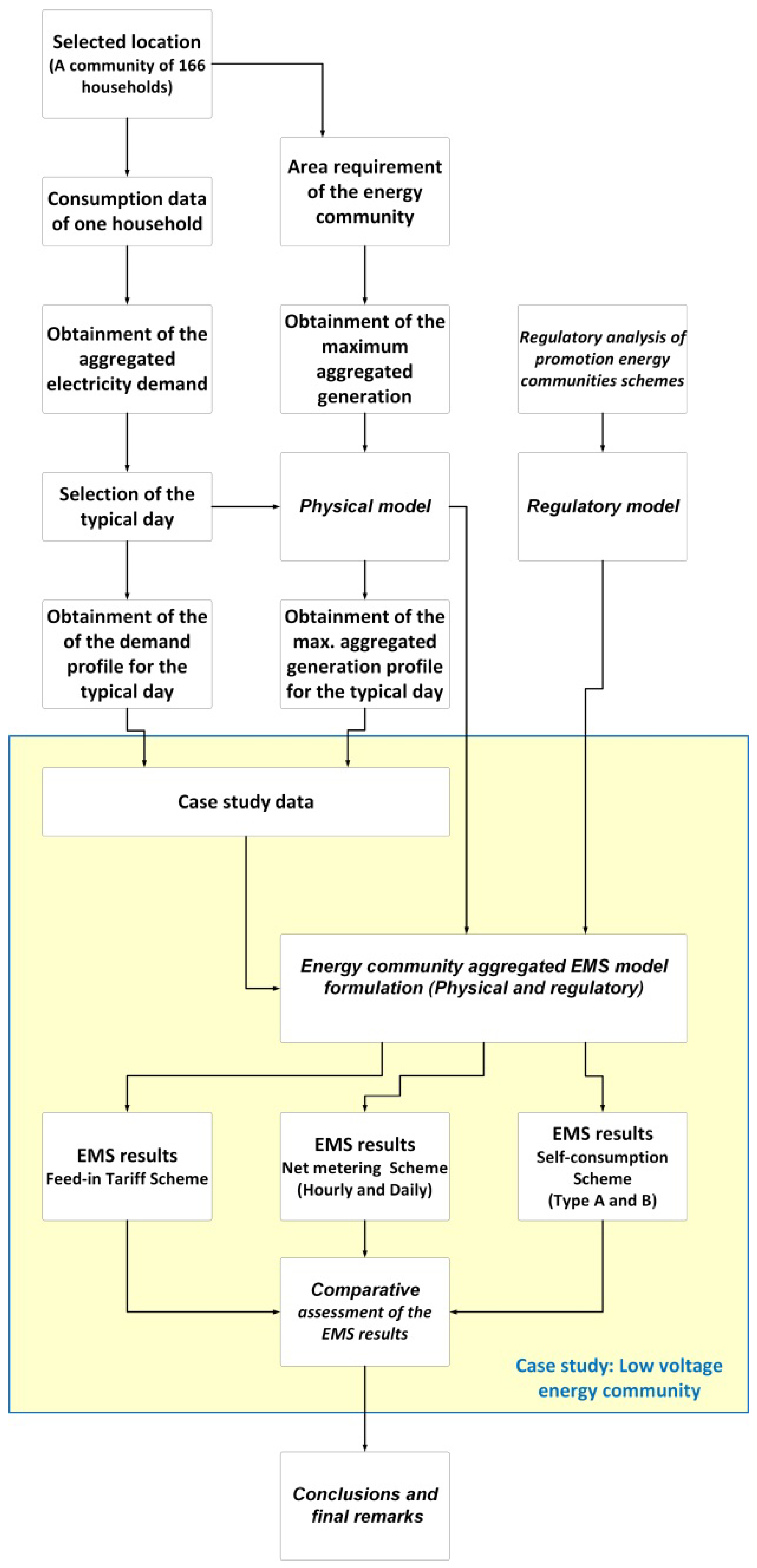
To the authors’ best knowledge, this is the first model which integrates regulatory constraints in a model addressed to optimize the energy management of an energy community, and compares the differences between different schemes.

1.3. Methodology

The methodology used to undertake the research was the following: Firstly, the problem was identified after an exhaustive search in the scientific literature. Once the topic has been defined and bounded, the main objective is stated: to prove the need of embedding regulatory structures into the mathematical model of an energy community as its economic results and the optimal energy management depend on them.

Next, two lines of action were taken. The first one tackles the physical model. An aggregated energy community model is formulated, including all balances of energy between renewable energy sources, consumptions and storage systems. Data of generation and demand of a specific site are gathered and processed according to the conception of the aggregated model. The second one tackles the regulatory models. Several regulations existing in European countries [30] are analyzed. The regulations are synthetized in order to represent its essence while avoiding their particularities. The energy bill structure is then formulated as the sum of electricity market prices, access tariffs, taxes, and charges. The billing and the energy retribution change depending on the regulatory structure applied.

The two lines of action are joined in a single optimization program which takes the form of a Mixed Integer Linear Program (MILP). The objective function is defined in economic terms, and several simulations are performed. Results are obtained for the different regulatory schemes in the same physical model, and conclusions are drawn. The methodology is summarized in Figure 1.

2. Model Description

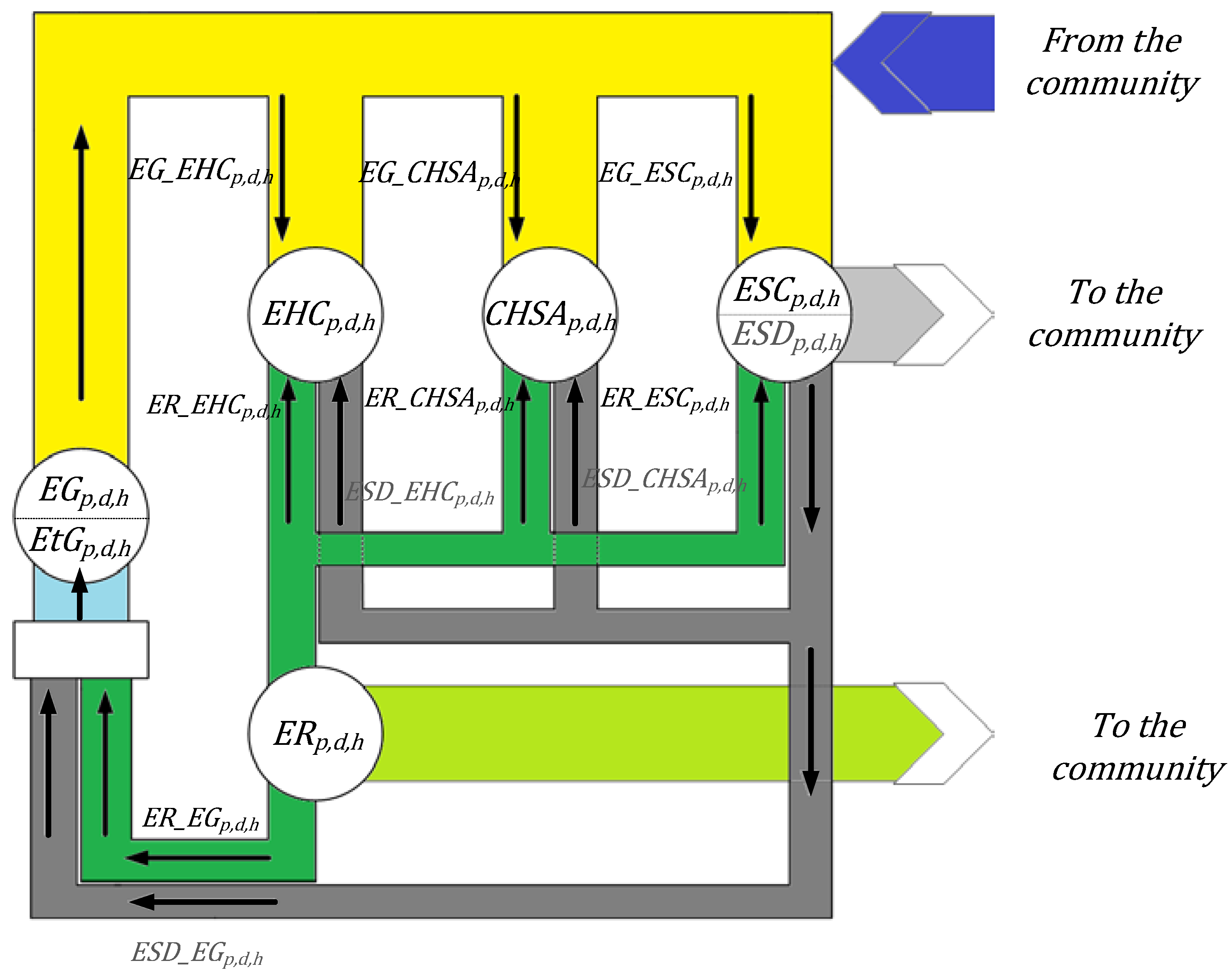
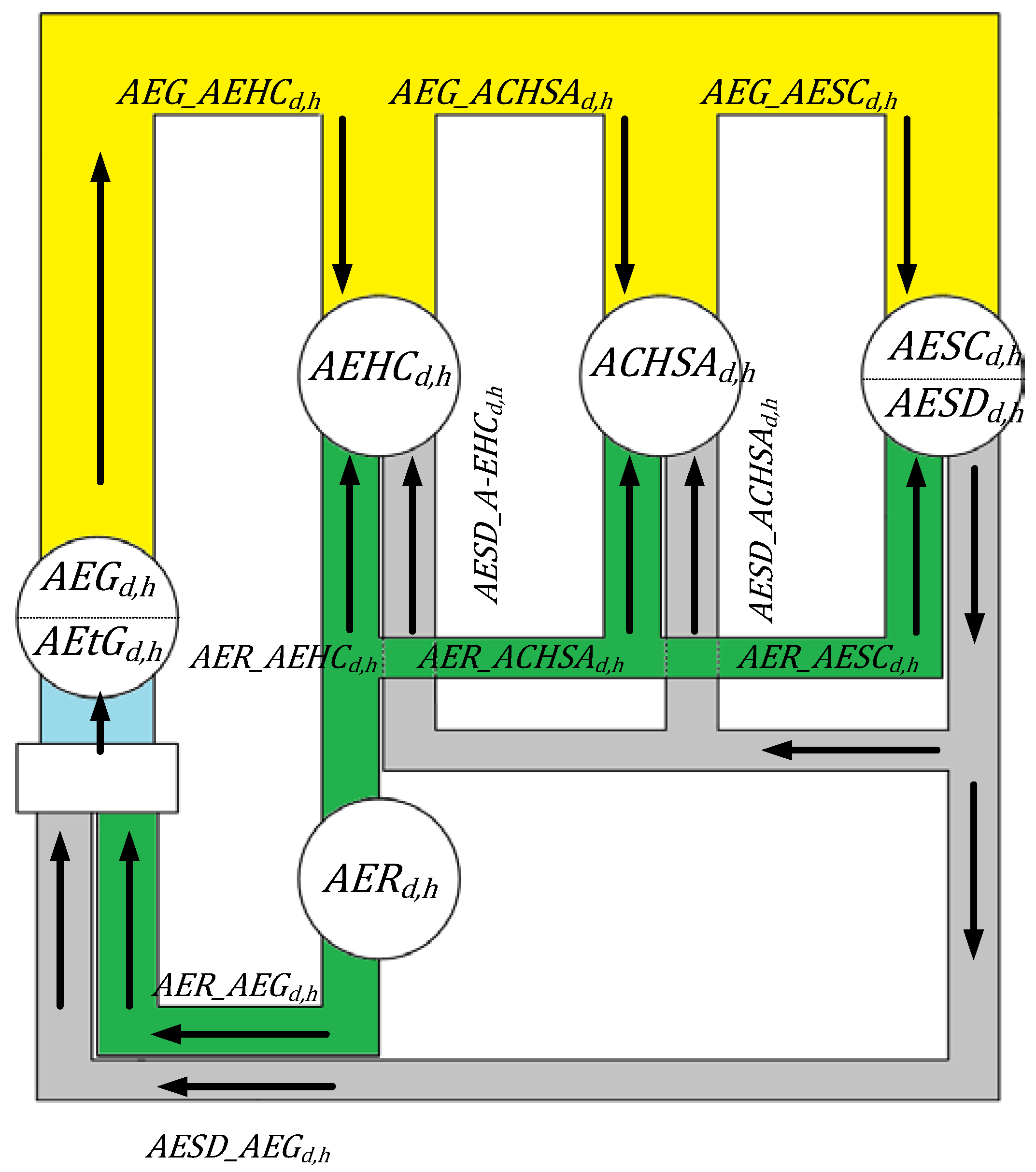
2.1. Physical Model

The physical model used is based on the work undertaken by de la Hoz et al. [34], but including the specificities derived from an energy community.

Each one of the prosumers that belong to the energy community is connected to the grid and possesses its distributed energy resources (DER), which in this case is a photovoltaic energy system, and an energy storage system (ESS). In this regard, each prosumer (p) can satisfy its energy demand using the grid, through the hourly (h) energy supplied by the network within a day (d) (EG_p,d,h). Likewise, the prosumer has at its disposal the hourly energy produced by its renewable energy resources within a day (ER_p,d,h), constrained to its maximum potential (ER_Max_p,d,h), and the hourly energy discharged within a day (ESD_p,d,h). The energy demand of a prosumer may be due to three types of consumption, namely, the hourly energy consumption within a day (EHC_p,d,h), the hourly auxiliary services consumption within a day (CHSA_p,d,h) and the hourly energy charged within a day (ESC_p,d,h). The EHC_p,d,h can be provided by the grid (EG_EHC_p,d,h), the renewable energy sources (RES) (ER_EHC_p,d,h) or the ESS (ESD_EHC_p,d,h). The same relation applies to the consumption of the ESS and the auxiliary services (ASS).

Additionally, each prosumer can help or be helped by the community. Additionally, they can inject its excess of energy to the grid (either from the RES (ER_EG_p,d,h) or from the ESS (ESD_EG_p,d,h)). All of these energy intricacies are depicted and summarized in Figure 2.

To obtain the physical model of the energy community, each one of the prosumer’s physical models that form the community was aggregated, resulting in the final energy community model. In this regard, as illustrated in Figure 3, the aggregation of all the RES and the ESS results in the aggregated hourly energy produced by the set of RES within a day (AER_d,h), the aggregated hourly energy discharged by the set of ESS within a day (AESD_d,h), and the aggregated hourly energy charged by the set of ESS within a day (AESC_d,h). Similarly, the aggregation of the consumption leads to the aggregated hourly energy consumption within a day (AEHC_d,h) and the aggregated hourly ASS consumption within a day (ACHSA_d,h).

2.2. Operating Costs

Operation and maintenance costs, O&M, are the necessary costs to keep a facility working during its whole lifetime. These costs can be fixed and variable. Fixed costs disregard whether the facility is not working or working at 100% of its capacity. An example of this cost could be, for a business, the rent of the property. Variable costs, on the other hand, are the ones which directly depend on the production of the facility. In the same business example these costs could include lighting or heating.

In PV generation, O&M costs correspond mostly to the maintenance of the generation elements with time and adverse weather conditions. These costs are eminently fixed, that meaning that they depend on the size of the facility and not on the amount of energy produced.

In the energy storage system, O&M costs also correspond to the maintenance of the batteries, but unlike PV generation, batteries present a cost due to their use. Therefore, both fixed and variable O&M costs are taken into account.

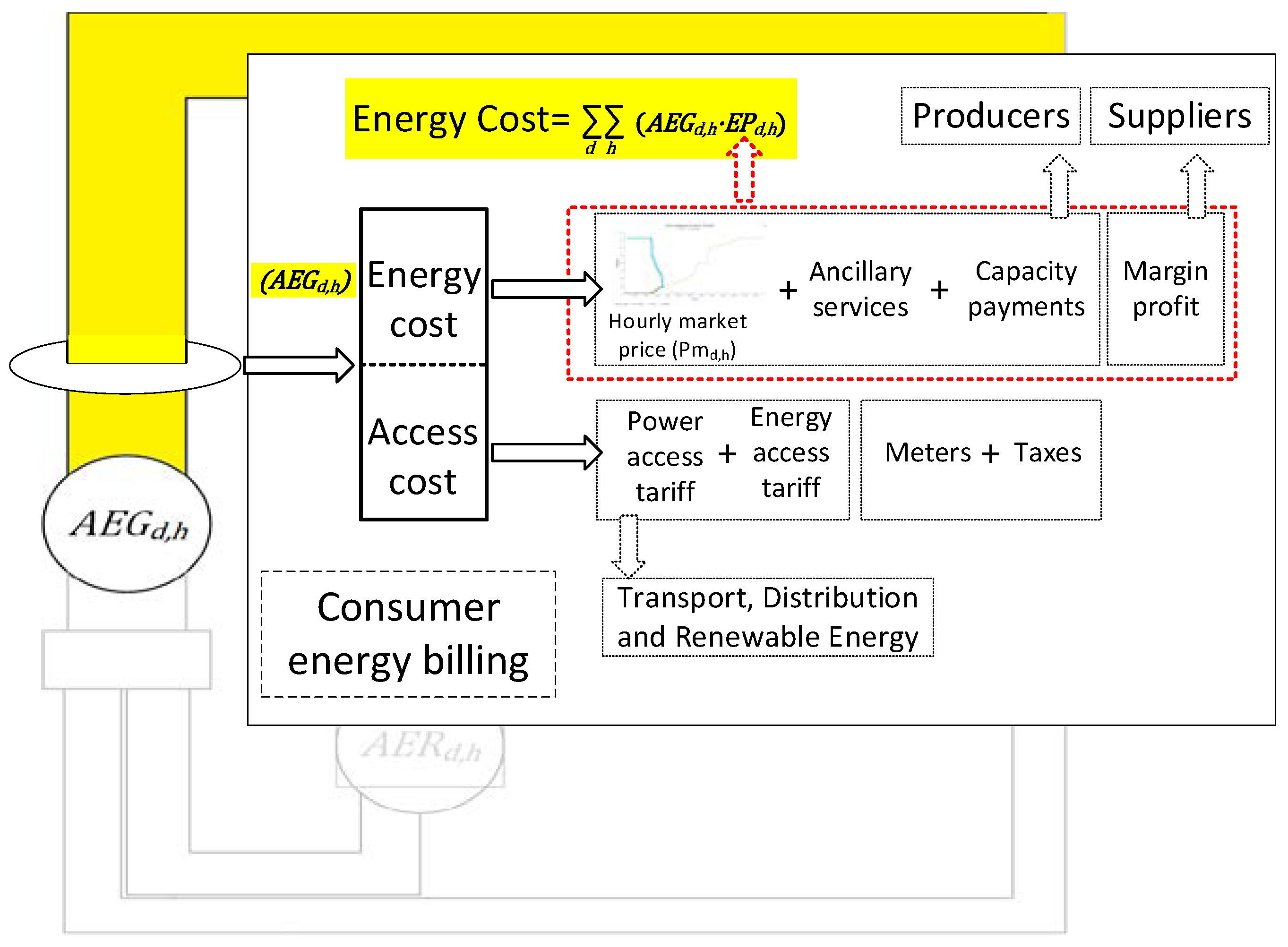
2.3. Consumers’ Energy Bill Structure

The formulation of the consumers’ electricity billing, without any kind of economic incentive, is based on the following concepts (see Figure 4). In the first place, there is the cost of energy; this cost covers all the expenses to produce the energy (including the day-ahead market price (Pm_d,h), ancillary services cost and capacity payments) plus a percentage to cover the energy loss (CEL) of the system. Moreover, the consumer has to face the supplier’s margin profit. As a result, the equivalent energy price that the consumer is facing (EP_d,h) is a little bit higher than just the market price.

The access cost is the second great term that impacts on the consumer’s electricity billing. Commonly neglected when defining the cost of supply, in this article comprises two terms; power term (Tp) and active energy term (Te). According to the rated power of the facility, these terms may have the same value through the day or have several values depending on the period defined. The article considered access terms with a single period (SP) value and with a three-time period (MP) value. The access cost covers the expenses of the transport and distribution networks, renewable energy promotion, and others. Finally, the third term is related to taxes and other fees, such as the meter rent. The taxes taken into consideration are the electricity tax and the VAT.

2.4. Consumers’ Energy Bill According to the Regulatory Structure Used to Promote Energy Communities

2.4.1. Setting the Context

According to Campos et al. [30], different types of regulatory schemes have been implemented to promote the development of energy communities in the European Union (EU). Among them, the most representative schemes are the Feed-In Tariff scheme, the Net Metering Scheme and the Self-consumption Scheme. A synthesis of these regulatory schemes was undertaken to determine their most representative characteristics and to obtain the basis of their regulatory structures concerning their remuneration mechanisms. In this regard, the following regulatory structures here depicted seek to represent the essence of each one of these regulatory schemes but avoiding particularities.

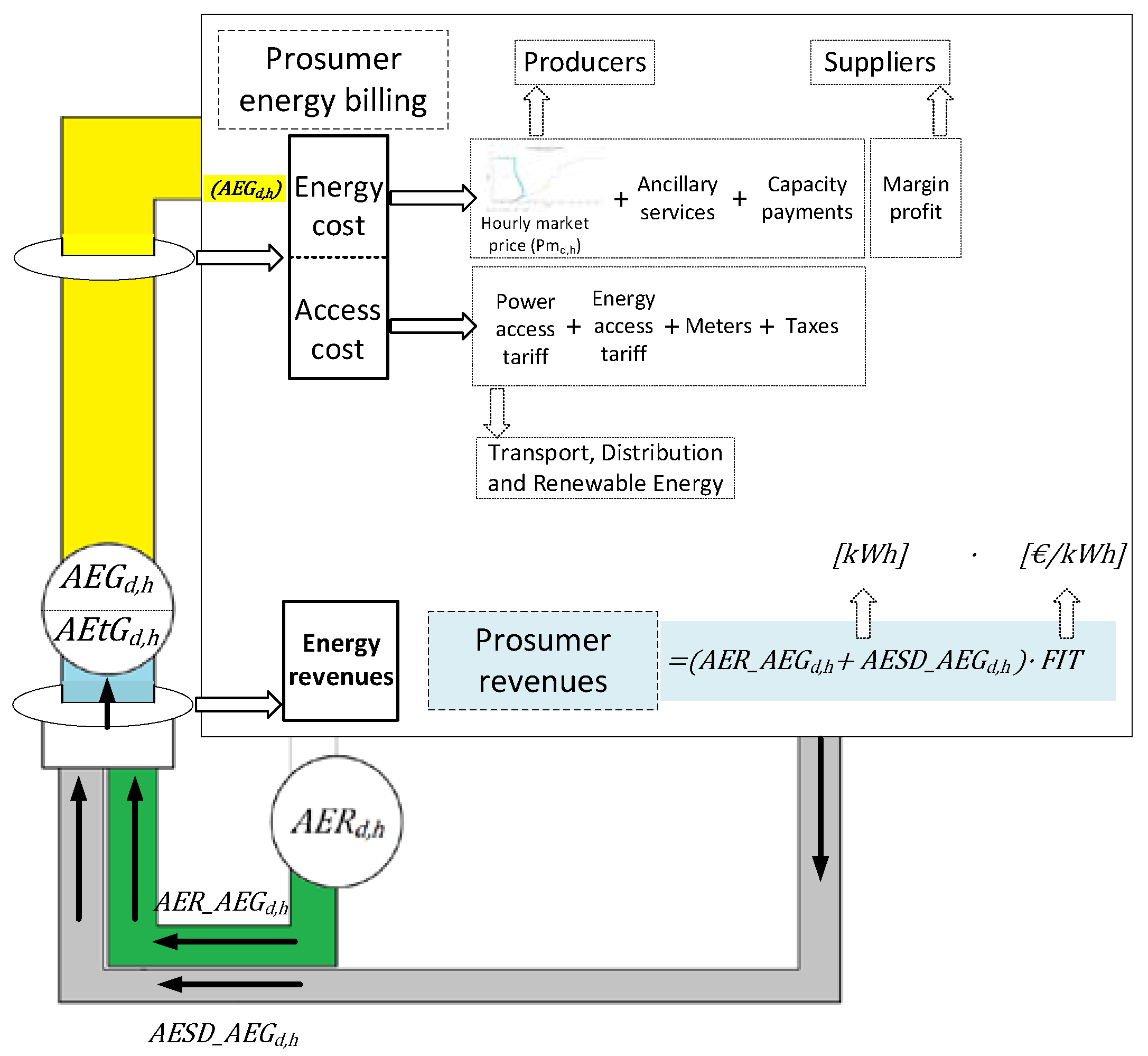
2.4.2. Feed-in Tariff

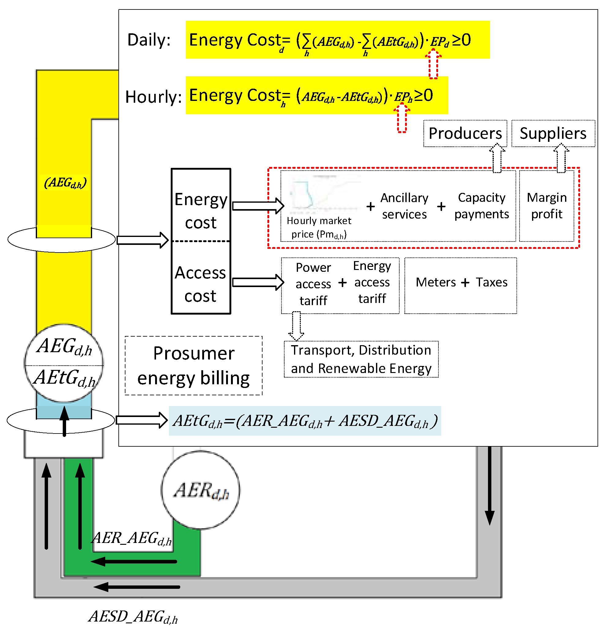
The most extended framework in the European Union is the Feed-in tariff. Originally, this system was designed for the energy which was fed into the grid, hence the name. Feed-in mechanisms impact the development of renewable energies by the use of a special tariff established by law.

Under a feed-in tariff (FiT) system, selected renewable energy producers perceive a quantity for the electricity that they feed into the grid, leading to the development of varied technologies and a reduced payback time. There are three key elements that define FiT. Firstly, the authority determines a minimum tariff for the sale of renewable electricity. This tariff changes depending on the source, size and location of the plant. FiTs normally decrease with time in order to promote technological change, but the tariff is fully disclosed in the beginning so investors can predict their remuneration during the whole lifespan of the project. Second, renewable producers see the access to the grid guaranteed by law, and third, the system is forced to purchase all of the electricity that is fed into the network [35].

For the FiT regulatory structure, as depicted in Figure 5, all the energy injected into the grid results in an income for prosumers.

2.4.3. Net Metering

Net metering is a system in which, like FiTs, a prosumer is rewarded for the energy that produces. Net metering is a structure which is specifically designed for self-consumption. In a system with net metering, the electric company introduces a meter that is bidirectional, meaning that it goes backwards if the generated electricity is superior to the consumed electricity. At the end of the billing period, which can be hourly, daily, monthly or even yearly, the consumer only pays for their net consumption, meaning the total aggregated energy consumption (AEG_d,h) minus the aggregated energy generation delivered to the grid (AEtG_d,h). In the study, the hourly and the daily net regulatory structure were synthesized as depicted in Figure 6.

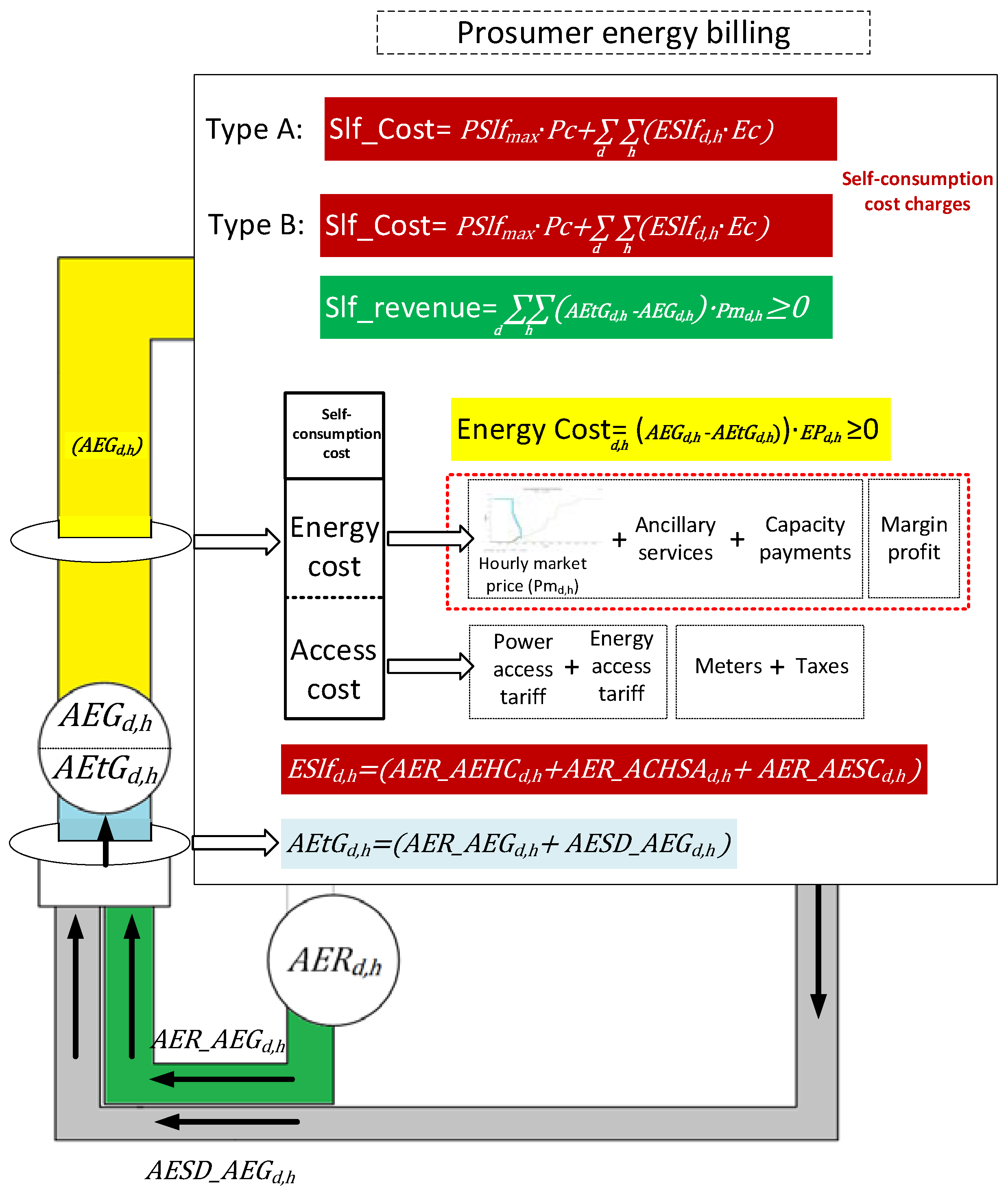
2.4.4. Self-Consumption

In this section, the main characteristics of the self-consumption structure used in this research are explained and defined (see Figure 7).

There are two modalities in the self-consumption structure. In the first modality (Type-A) the prosumer is not rewarded for the fed energy into the grid. The other modality (Type-B) is quite the contrary. In any case, the rated power of the RES does not surpass the rated power of the supply.

As happens with the net metering structure, the cost of energy under the self-consumption structure is diminished as the prosumer injects the self-produced energy into the grid (Type-B). Nevertheless, the self-produced energy is charged through two terms, the power charges (Pc) and the energy charges (Ec).

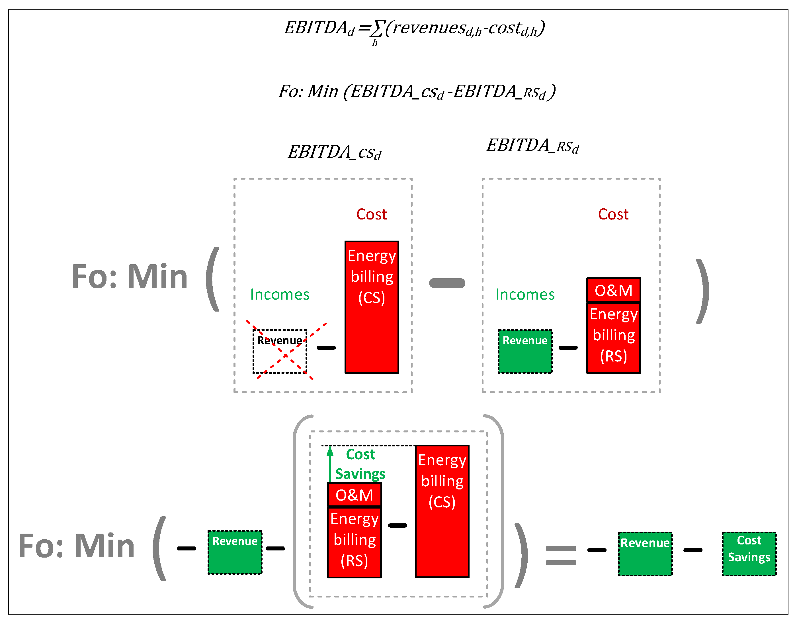
2.5. Objective Function

The primary goal of an energy management system (EMS) is to ensure the most economical operation for the end-users, meaning the inhabitants of the energy community. The distributed generation facility would make no sense in the case that its operation was more expensive than to operate with a conventional system.

The installation of RES under any type of regulatory structure addressed to promote energy communities reduces, in theory, the electrical bill; thus, it induces a reduction in the operating costs. The Earnings Before Interests, Taxes, Depreciation and Amortization indicator (EBITDA) is used to calculate the magnitude of the savings.

These savings are determined by comparing the value of the EBITDA of the energy community with and without RES. Therefore, the objective function will then contrast the EBITDA under the regulatory structure (EBITDA_RS) with the EBITDA in the conventional system (EBITDA_CS), for the planning horizon considered in the mathematical program. In this case, the objective function was formulated as the minimization of the difference between EBITDA_CS and EBITDA_RS, which is equivalent to maximizing the community savings; thus, its expression is the following:

Obj.f ≔ min (EBITDA_CS − EBITDA_RS)

(1)

2.6. Constraints

2.6.1. Energy Balances and Limits

Constraints are expressions which restrict the values that variables can have in order to allow the program to have a definite solution. Several of them ensure that that the aggregated balances of energy are fulfilled:

AEHC_d,h = AEG_AEHC_d,h + AER_AEHC_d,h + AESD_EHC_d,h

(2)

ACHSA_d,h = AEG_ACHSA_d,h + AER_ACHSA_d,h + AESD_ACHSA_d,h

(3)

AESC_d,h = AEG_AESC_d,h + AER_AESC_d,h

(4)

AEtG_d,h = AER_AEG_d,h + AESD_AEG_d,h

(5)

AESD_d,h = AESD_AHCSA_d,h + AESD_AEHC_d,h + AESD_AEG_d,h

(6)

AER_d,h = AER_AHCSA_d,h + AER_AEHC_d,h + AER_AEG_d,h + AER_AESC_d,h

(7)

AEG_d,h = AEG_AHCSA_d,h + AEG_AEHC_d,h + AEG_AESC_d,h

(8)

The exchange from (or to) the grid is characterized as follows:

Ex_Grid_d,h = AEG_d,h − AEtG_d,h

(9)

The exchange from (or to) the set composed by the RES and the ESS is also defined as follows:

Ex_ RES_ESS_d,h = AEG_CHSA_d,h + AEG_AESC_d,h − AER_AEHC_d,h − AER_AEG_d,h − AESD_AEHC_d,h − AESD_AEG_d,h

(10)

Limits on generation and storage capacity must be imposed. Moreover, a parameter which defines the existence or not of battery systems is introduced:

AER_p,d,h ≤ AER_max_p,d,h

(11)

S_p,d,h ≤ Smax_p

(12)

$$\mathrm{AESD}\_{\mathrm{ACHSA}}_{\mathrm{p},\mathrm{d},\mathrm{h}}+\mathrm{AESD}\_{\mathrm{AEHC}}_{\mathrm{p},\mathrm{d},\mathrm{h}}+\mathrm{AESD}\_{\mathrm{AEG}}_{\mathrm{p},\mathrm{d},\mathrm{h}}\le \mathrm{M}\times \mathrm{Binary}\_{\mathrm{St}}_{\mathrm{p}};\mathrm{M}\to \infty$$

(13)

2.6.2. Energy Storage Constraints

The mathematical model to represent the battery is based on the article by Luna et al. [36]. The article observes that the battery energy storage system must be charged in two phases in order to avoid overload and maintain its lifespan. In the first phase, battery ESS interacts normally with the grid until the cell voltage reaches a so-called regulation voltage. After that, the second phase takes place, in which the voltage is set to its regulation value, but the current is asymptotically reduced to 0. In this second phase, battery ESS stops interacting with the grid and limits the charge power to a certain value in order to keep the voltage constant.

The transition between phases is introduced in the program with the binary variable Status. When Status has a value of 0, the battery is operative and interacts normally with the grid; on the other hand, a Status 1 means that the battery has reached the regulation voltage, is almost charged, and therefore the interactions with the grid and the charge power are limited.

SoC_d,h ≤ SoC_th + (SoCmax-SoC_th) × Status_d,h

(14)

SoC_d,h ≥ SoCmin + (SoC_th-SoCmin) × Status_d,h

(15)

PSC_d,h ≤ PSC_Th + (PSCmax-PSC_Th) × (1-Status_d,h)

(16)

PSD_d,h ≤ PSD_Th + (PSDmax-PSD_Th) × (1-Status_d,h)

(17)

$$\mathrm{EG}\_{\mathrm{ESC}}_{\mathrm{d},\mathrm{h}}\le \mathrm{M}\times (1-{\mathrm{Status}}_{\mathrm{d},\mathrm{h}});\mathrm{M}\to \infty$$

(18)

Additionally, other constraints are imposed on the battery to increase its lifetime. Given the depth of discharge (DoD) as the difference between the maximum and minimum state of charge of the battery, the specifications of most manufacturers recommend DoD to be less than or equal to 80% for a correct operation of the battery. Nevertheless, DoD must not be very small, because it limits the storage capacity of the battery and thus the number of cycles needed for normal operation becomes higher. This, in turn, can reduce the lifespan of the battery. In consequence, the value of DoD is set at 80%.

The battery state of charge is defined and updated as following. Additionally, a constraint is imposed, such as the state of charge not being reduced by the end of the simulation period.

SoC_p,d,h = S_p,d,h/Smax_p,

(19)

S_p,d,1 = S0

(20)

S_d,h = S_d,h-1 + ESC_d,h × Nbat-ESD_d,h/Nbat×

(21)

$$\sum _{\mathrm{h}=1}^{23}{\mathrm{SoC}}_{\mathrm{d},\mathrm{h}+1}-{\mathrm{SoC}}_{\mathrm{d},\mathrm{h}}\ge 0$$

(22)

2.6.3. Energy Costs and Billing Constraints

The billing procedure is synthetized by the following constraints:

$$\mathrm{Energy}\_{\mathrm{Cost}}_{\mathrm{p},\mathrm{d},\mathrm{h}}={\mathrm{Tp}}_{\mathrm{p}}\times {\mathrm{PCon}}_{\mathrm{p}}+{\sum }_{\mathrm{d},\mathrm{h}}({\mathrm{AEG}}_{\mathrm{p},\mathrm{d},\mathrm{h}}·{\mathrm{Te}}_{\mathrm{p},\mathrm{h}})+{\mathrm{AEG}}_{\mathrm{p},\mathrm{d},\mathrm{h}}\times {\mathrm{EP}}_{\mathrm{d},\mathrm{h}}$$

(23)

And variables related to the operation and maintenance costs of the facility are defined as:

CFG_AU_p = CFG × max_d,h(AER_p,d,h)

(24)

$$\mathrm{CVG}\_{\mathrm{AU}}_{\mathrm{p}}={\sum }_{\mathrm{d},\mathrm{h}}{\mathrm{AER}}_{\mathrm{p},\mathrm{d},\mathrm{h}}·\mathrm{CVG}$$

(25)

CF_ST_p = max_d,h(PSD_p,d,h + PSC_p,d,h) × CFS

(26)

$$\mathrm{CV}\_{\mathrm{ST}}_{\mathrm{p}}={\sum }_{\mathrm{d},\mathrm{h}}({\mathrm{ESD}}_{\mathrm{p},\mathrm{d},\mathrm{h}}+{\mathrm{ESC}}_{\mathrm{p},\mathrm{d},\mathrm{h}})\times \mathrm{CVS}$$

(27)

C_GAU_p = CFG_AU_p + CVG_AU_p + CF_St_p + CV_St_p + IMP_GE_p

(28)

Finally, the taxes related to the energy sale are the following:

$$\mathrm{IMP}\_{\mathrm{ENG}}_{\mathrm{p}}=\mathrm{ENG}·{\sum }_{\mathrm{d},\mathrm{h}}{\mathrm{AEtG}}_{\mathrm{d},\mathrm{h}}$$

(29)

3. Case study

3.1. Physical Conditions

Data regarding electrical consumption were gathered from a household located at the geographic coordinates 41,65N, 2,16E. This dwelling belongs to a residential area consisting of 166 dwellings of similar characteristics. The energy community considered in this study corresponds to this area. In the following points, the physical input data required by the model is depicted, described in Section 2.

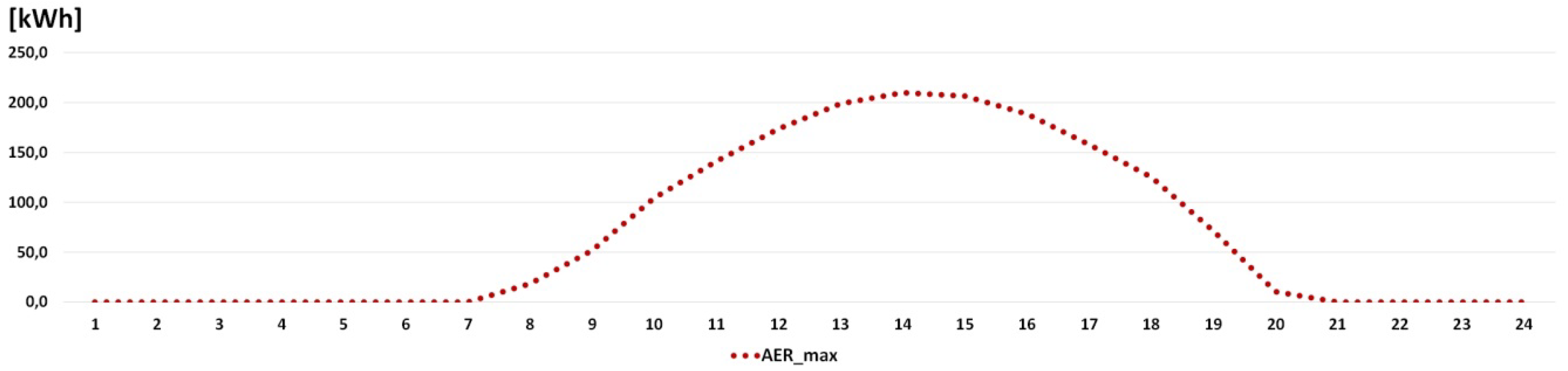
3.1.1. Maximum Aggregated Energy Produced by the Energy Community

The following steps were conducted in order to determine the AER_max_d,h, namely the maximum aggregated hourly energy produced by the set of RES within a day.

First of all, the study of the area requirement was undertaken for all households. The resulting photovoltaic area was restricted to the available area of each household. An optimal tilt of 37° was considered for each household, regardless of its Azimuth. The PVGIS application was employed [37] to estimate solar radiation. In order to adapt the PVGIS time system (solar time) to UTC, 0.14 h were subtracted. Subsequently, one or two hours were added depending on the month to account for the corresponding time zone (UTC + 1 in winter and UTC + 2 in summer).

The maximum energy produced for the most representative day of each month, and each household, was determined using generic models from the PVSyst database [38] of PV modules and inverters. Next, the aggregated maximum energy produced by the energy community for the most typical day of each month was determined. The selection of the typical day to be studied is based on this energy. The typical day to be studied is a typical day of September. It was chosen as a trade-off between the most and least favorable energy production situation. The maximum aggregated energy produced by the energy community for the most typical day of September is depicted in Figure 8.

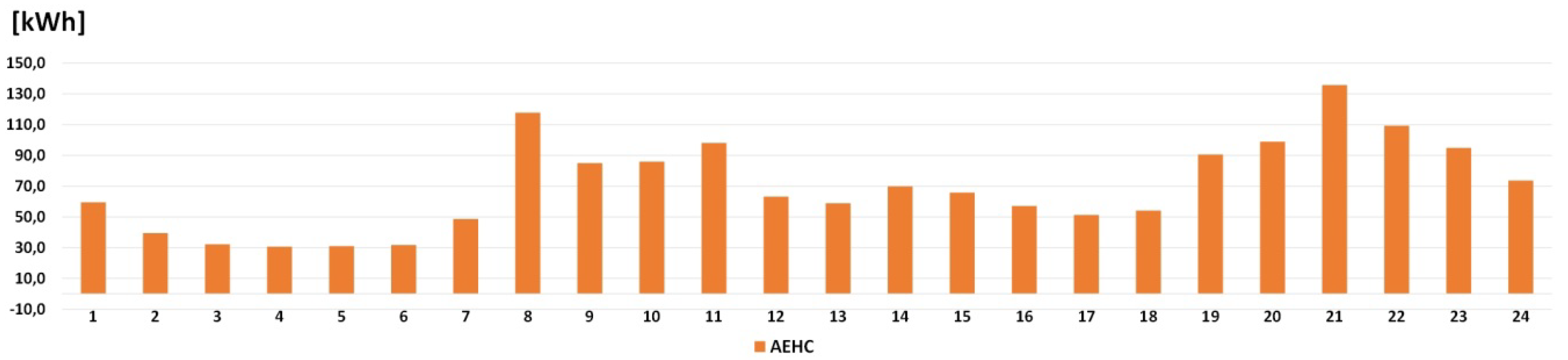
3.1.2. Aggregated Hourly Energy Consumption of the Energy Community

The available data of energy consumption consist of the hourly consumption of 1 of the 166 dwellings of the community. Averaging the data for all the days and then multiplying them by the number of households to generate the overall consumption is not useful, because the result does not show a representative consumption profile. The mean consumption tends to be more constant in time than the typical consumption of a single dwelling, which has ups and downs.

The method described by Ortiz et al. [39] was used to obtain the community’s demand profile based on the data of a single dwelling. In this method, profiles of consumption for different households are created based on the probability of use of the most common electrical appliances. These probabilities ${\mathrm{p}}_{\mathrm{e},\mathrm{d},\mathrm{h}}$ are calculated in [40]. Firstly, a combination of appliances ${\mathrm{N}}_{\mathrm{e}}$ according to available data of the household consumption is found.

$$\min \left(\sum _{\mathrm{e},\mathrm{d}}{\mathrm{p}}_{\mathrm{e},\mathrm{d},\mathrm{h}}{\mathrm{N}}_{\mathrm{e}}{\mathrm{P}}_{\mathrm{e}}-\sum _{\mathrm{d}}{\mathrm{EHC}}_{\mathrm{data},\mathrm{d},\mathrm{h}}\right)$$

(30)

Then, based on the aforementioned probabilities of use, it is assumed that every household in the community has the same appliances ${\mathrm{N}}_{\mathrm{e}}$, but different habits of consumption. These different habits of consumption are represented by a random number ${\mathrm{R}}_{\mathrm{e},\mathrm{d},\mathrm{h}}$ under the following conditions:

• If ${\mathrm{R}}_{\mathrm{e},\mathrm{d},\mathrm{h}}>{\mathrm{P}}_{\mathrm{e},\mathrm{d},\mathrm{h}}$ the appliance is on stand-by and consumes a minimal power.
• Otherwise, if ${\mathrm{R}}_{\mathrm{e},\mathrm{d},\mathrm{h}}\le {\mathrm{P}}_{\mathrm{e},\mathrm{d},\mathrm{h}}$ the device is on and consumes an energy equal to ${\mathrm{P}}_{\mathrm{e}}·\mathsf{\Delta }\mathrm{t}$, with $\mathsf{\Delta }\mathrm{t}$ the time step
• ${\mathrm{R}}_{\mathrm{e},\mathrm{d},\mathrm{h}}$ is generated with a standard uniform distribution between 0 and 1 and e is only evaluated for the combination of appliances ${\mathrm{N}}_{\mathrm{e}}$ previously found.

For each 1 of the 166 dwellings, according to Equation (30), a set of random numbers ${\mathrm{R}}_{\mathrm{e},\mathrm{d},\mathrm{h}}$ is generated and their individual profiles are obtained by summing all the power consumed by their appliances. This leads to every dwelling having different peak consumption hours, and thus, to the overall sum being more realistic.

The aggregated hourly energy consumption for the typical day of September is depicted in Figure 9.

3.1.3. Battery Model

The battery characteristics are also extracted from the generic database of PVSyst for the Pb-Lead technology, and its values are depicted in

Table 1. Battery model data.

Aggregated battery capacity	1275 kWh
Aggregated maximum charge/discharge power	127.5 kW
Aggregated maximum charge/discharge power at status 1	25.5 kW
Efficiency	1 (ideal)

.

3.2. Economic Conditions

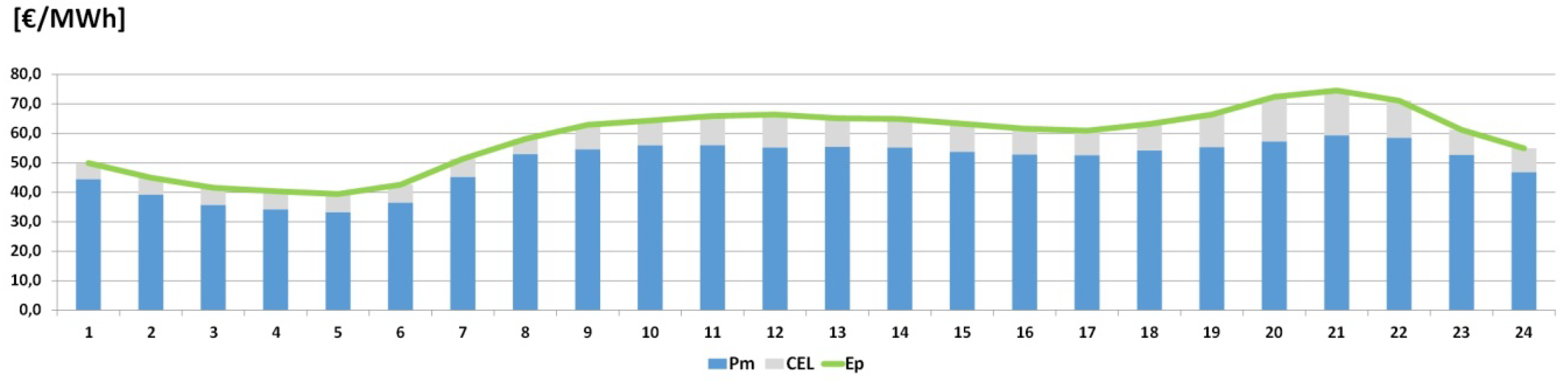
3.2.1. Electricity Market Prices

The electricity price for a typical weekday day of September was obtained from the Iberian Spot Power Market Operator database [41] over the last few years. As a result, Figure 10 depicts the day-ahead market price, the cost of the energy loss of the system and the equivalent energy price of the consumer.

3.2.2. Electricity Billing Access Tariffs

The data of the access tariffs used for the analysis is depicted in

Table 2. Access tariff coefficients [42].

Type of Supply Contract	Single Period (SP)	Multiple Period (MP)
Access tariffs	p = 1	p = 1	p = 2	p = 3
Te [€/kWh]	0.044	0.062	0.003	0.001
Tp [€/kW·year]	38.04	38.04	38.04	38.04

.

3.2.3. Electricity Billing under Feed-in Tariff and Net Metering

Both feed-in tariff and net-metering schemes follow very simple variations in respect to the billing without self-consumption. In the case of feed-in tariff, the price of energy sale is fixed, disregarding the amount of energy sold, the location of the facility and the time of the year. In this paper, the feed-in tariff value is fixed to 0.1315 €/kWh.

Under a net metering scheme, there is no price for the sale of energy, but every unit of energy sold into the grid discounts one unit of energy imported from the grid. In consequence, the amount of energy taken into account at the bill is equal to the purchased energy minus the sold energy, with the condition that this amount can never be negative.

3.2.4. Electricity Billing under Self-Consumption Regulatory Structure

Regarding the self-consumption regulatory structure, besides the well-known costs (energy cost and access cost), some additional charges are also included in the energy billing. These charges are justified, under this scheme, because self-consumption compromises the stability of the grid.

The values of the additional charges used in the article are depicted in

Table 3. Self-consumption charges [43].

Type of Supply Contract	Single Period (SP)	Multiple Period (MP)
Charges	p = 1	p = 1	p = 2	p = 3
Ec [€/kWh]	0.043	0.058	0.006	0.006
Pc [€/kW·year]	8.144	8.144	8.144	8.144

.

3.2.5. O&M Costs

The value of the cost of the aggregated PV systems was extracted from the Spanish Renewable Energy Plan [44] and they amount to 35.6 €/kW.

Concerning the aggregated ESS cost, both fixed and variable, these are extracted from the article of Zakeri and Syri [45], where an exhaustive analysis of different technologies of energy storage is realized. Moreover, a statistical breakdown of costs is included. In this regard, the mean cost used in their research is employed. It has to be taken into account that these costs have a strong dependence on the operational regime of the batteries. In the aforementioned article, costs are calculated for a DoD of 80%. The same conditions apply in this case.

3.3. Data Summary

The data employed in the simulation for a typical weekday of September is summarized in

Table 4. Data employed for the energy community simulation.

Data	Value and Units
Time step	1 h
Simulation day	Typical day of September
Generation and consumption
Peak consumption	135.7 kW
Hour of peak consumption	21 h
Daily consumed energy	1683 kWh
Auxiliary services consumption	1.66 kW
Contracted power	381.3 kW
PV peak power per dwelling	2.25 kW
Aggregated PV peak power	209.8 kW
Aggregated generated energy	1657 kWh
Energy storage
Aggregated battery capacity	1275 kWh
Aggregated maximum charge/discharge power	127.5 kW
Aggregated maximum charge/discharge power at status 1	25.5 kW
Efficiency	1 (ideal)
Depth of discharge	80%
Initial State of Charge	60%
Electricity billing
Meter rent	1.11 €/month
VAT	21%
Electricity tax	5113%
Electricity market price	0.039–0.075 €/kWh
Power term of the access tariff	38.04 €/kW·year
Energy term of the access tariff	0.002–0.062
Feed-in Tariff	0.135 €/kWh
Self-consumption O&M Costs
Energy sale tax	0.5 €/MWh + 7% over the energy value
PV O&M costs	36.1 €/kW·year
Storage O&M costs	6.1 €/kW·year + 0.49 €/MWh

.

4. Results

4.1. Energy Management Results with ESS

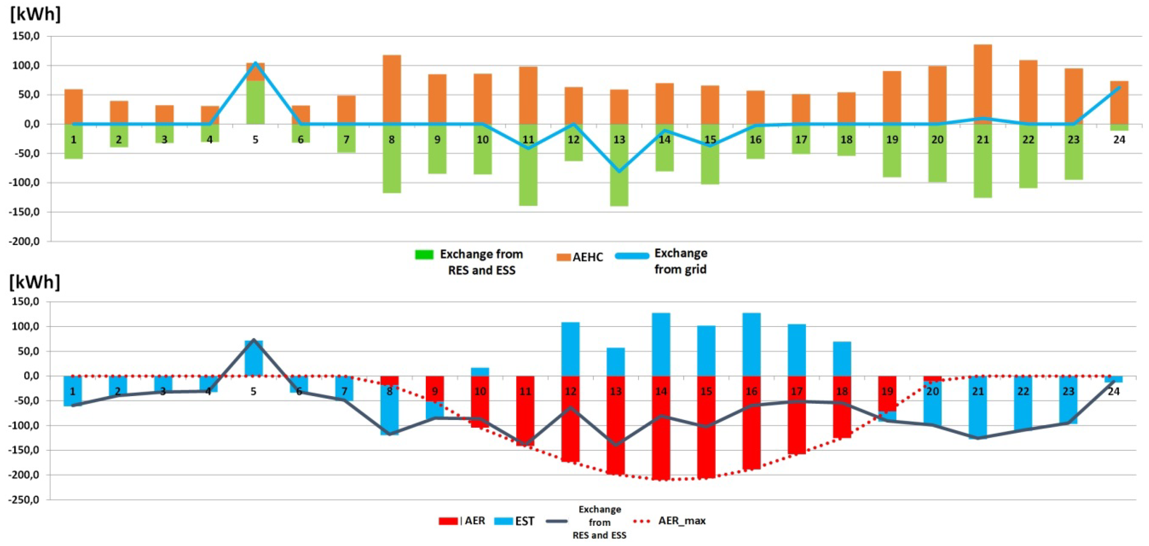
4.1.1. Feed-in Tariff Scheme

Under a FiT scheme, the optimal solution leads to a continuous injection of energy into the grid, except for the energy that is necessary to satisfy the customer’s needs. It indicates that the value of the FiT is high enough to prioritize the injection of electricity from renewable sources (RES_E) to the grid rather than to store it to compensate for the fluctuation of the electricity price. This is the reason why, as depicted in Figure 11, the charge of the batteries is concentrated between 2 a.m., and 7 a.m., during the period with the lowest energy prices. This stored energy is finally used to satisfy the consumption of the energy community at the end of the day, avoiding the highest equivalent energy prices.

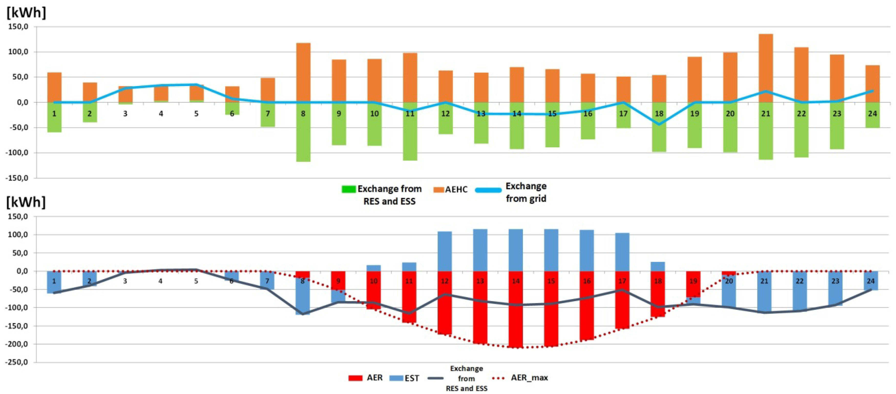
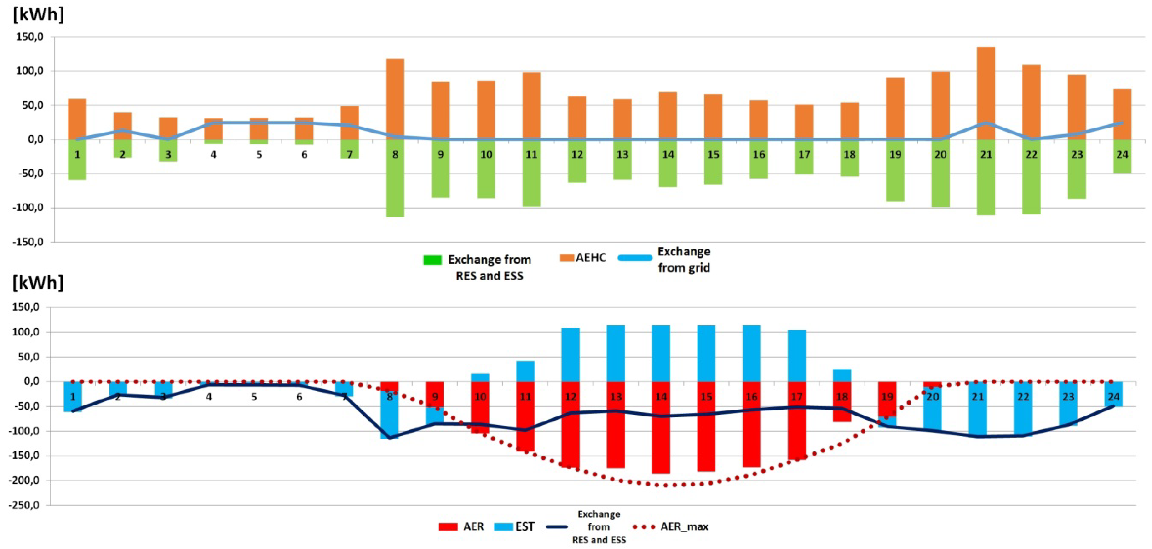
4.1.2. Net Metering Results

Under the net metering scheme, all of the generated energy is almost used up in supplying the energy to the aggregated energy consumption and storage. As the remuneration for injecting energy no longer rules, the exchange to the grid, mostly between 12 a.m. to 4 p.m., is substantively reduced (see Figure 12 and Figure 13). This fact leads the EMS to use the RES_E to charge the ESS. This RES_E is used at the end of the day to feed the aggregated energy consumption of the energy community. As a result, battery use under the net metering scheme is more intensive than under the FiT scheme.

In terms of EMS, when comparing both net-metering schemes, it should be highlighted that the daily net-metering scheme could allow the EMS better prevention of sharp interactions of exchange of energy with the grid.

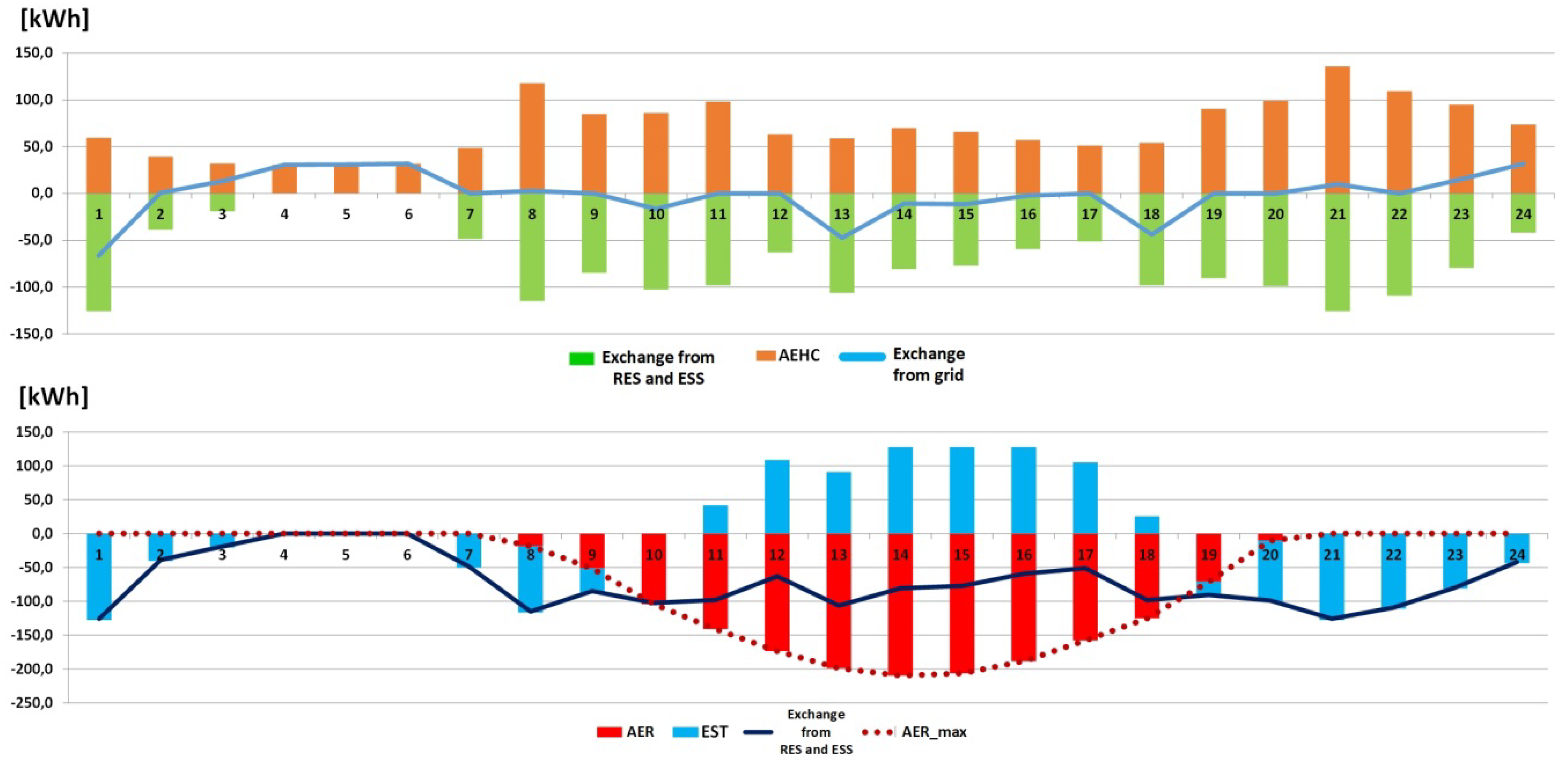
4.1.3. Self-Consumption Results

Despite the differences, energy management under the Type-B self-consumption scheme is quite similar to the energy management results under the net metering scheme. Under this scheme, the injection of energy to the grid is permitted and rewarded. In this regard, and despite the charges applied to self-consumed energy, there is a positive economic balance when the value of the difference between the day-ahead market energy price and the charges is positive. Therefore, the EMS uses this fact in order to optimize the economic results (see Figure 14).

Unlike Type-B, Type-A self-consumption scheme presents significant differences when managing the energy community when compared with the other schemes. The energy management is mainly addressed to optimize energy savings. Due to the injection of energy to the grid is not rewarded and, because there is a charge for the self-consumed energy, the maximum aggregated energy produced by the energy community is not entirely used. The energy only is produced and stored if it results in an economic saving (see Figure 15).

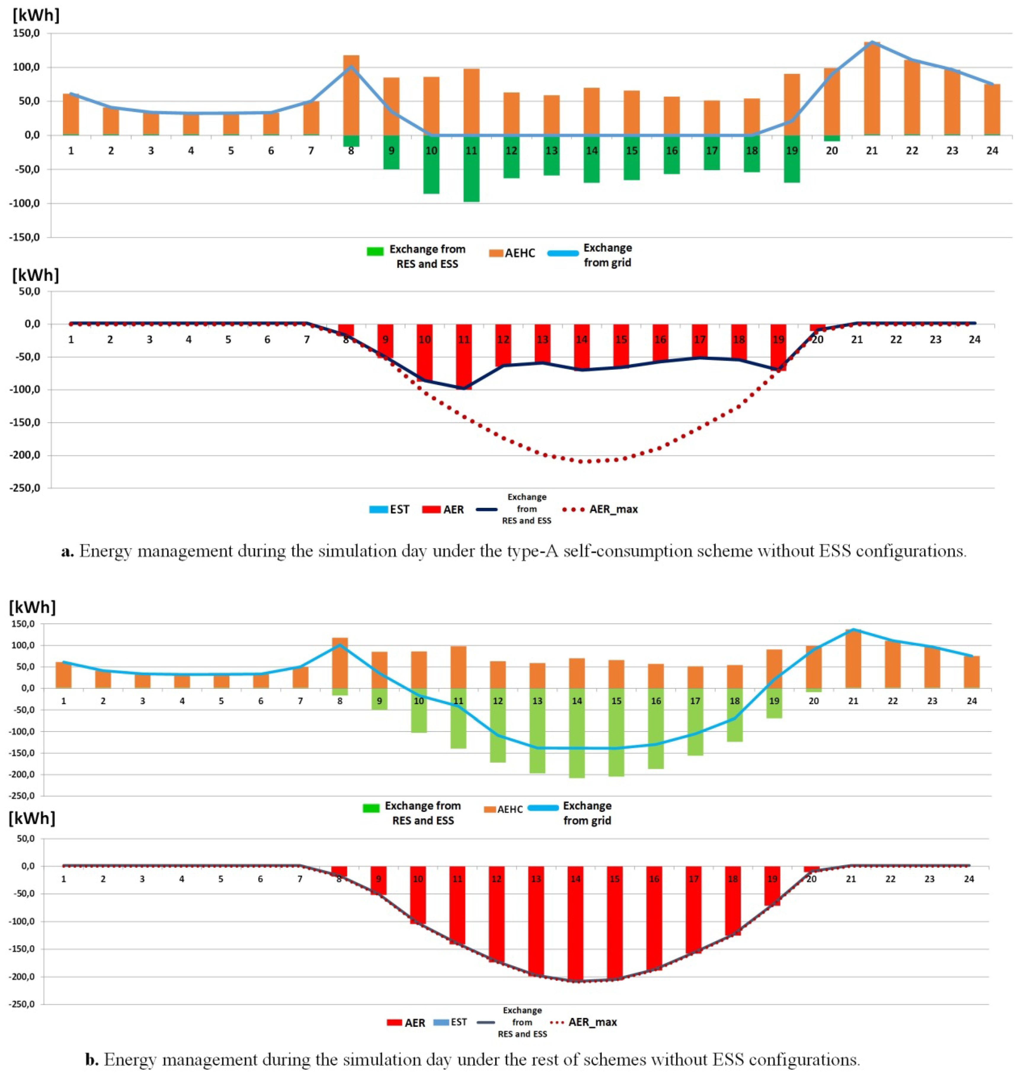
4.2. Energy Management Results without ESS

The energy management of an energy community is significantly affected if the ESS is not used. In this case, for all the promotion schemes but the Type-A self-consumption, the energy management result is the same. For the Type-A self-consumption scheme, the charges for the self-produced energy and the lack of economic reward for injecting this energy into the grid result in the lowest aggregated hourly energy produced by the energy community. The energy produced is addressed to supply the aggregated hourly energy consumption of the energy community exclusively (see Figure 16a).

In the rest of schemes—as they either allow for the compensation of the injected energy into the grid with the energy consumption, or they receive remuneration for it—the system is forced to inject all the maximum aggregated energy produced into the grid to optimize the economic results (see Figure 16b).

4.3. Economic Results

The optimal energy management led to an optimal economic result. These results are depicted in

Table 5. The Objective function and overall saving results [€/day] for the energy community under different regulatory schemes *.

			Energy Community with ESS					Energy Community without ESS
Type of Scheme		Type of Scheme	FiT	DNM	HNM	SF_B	SF_A	FIT	DNM	HNM	SF_B	SF_A
Type of supply	SP	O. F. value	−1.31	−1.19	−1.10	−0.60	−0.56	−1.14	−0.84	−0.48	−0.15	0.07
		Overall saving results	1.31	1.19	1.10	0.60	0.56	1.14	0.84	0.48	0.15	−0.07
	MP	O. F. value	−1.80	−1.07	−0.98	−0.65	−0.60	−1.17	−0.85	−0.45	−0.29	−0.07
		Overall saving results	1.80	1.07	0.98	0.65	0.60	1.17	0.85	0.45	0.29	0.07

* SF_A: self-consumption scheme type-A. SF_B: self-consumption scheme type-B. DNM: daily net metering. HNM: hourly net metering.

. In this regard, at first sight, it is obvious how, according to different regulatory structures, these economic results may differ in value. Therefore, a better understanding of the objective function might be required to have a clear insight into how the regulatory structures could affect the economic results (see Figure 17).

The EBITDA, which considers the revenues and the costs related to any economic activity, is the basis of the objective function. This function is defined as the difference between the EBITDA of the conventional system (EBITDA_CS) and the one under the regulatory framework (EBITDA_RS).

In the conventional case, namely without RES, the household community does not have any type of revenues, only the cost of its energy supply. When the household community becomes an energy community, being able to produce its own energy, the resulting EBITDA changes. Depending on the regulatory structure applied, the energy community might see the energy produced rewarded and the energy bill reduced. Moreover, due to the existence and operation of the RES, an operation and maintenance cost also appears.

By minimizing the objective function, it is sought to increase the economic savings introduced by the RES. This objective can be achieved if the revenues, savings, or both, increase. The lower the objective function, the higher the savings for the energy community.

5. Discussion

5.1. Regarding the Energy Management and the Economic Results of the Energy Community

The economic results corroborate the importance of embedding the economic intricacies of the regulatory structures into the algebraic model addressed to optimize the energy management of the energy community. As it was proved, different regulatory schemes resulted in different energy management results. The differences in the energy management results are summarized in

Table 6. Summary of the differences in energy management under different regulatory schemes.

Type of Scheme	Main Features of the Energy Management
FiT	Maximises the electricity dump into the grid. Favourable hourly discrimination Reduced energy storage use
HNM	Electricity dump mainly without ESS Unfavourable hourly discrimination Extensive use of energy storage. A significant difference between using ESS or not
DNM	Similar management to hourly net metering Neuter hourly discrimination Extensive use of energy storage but the differences are not so significant.
SF_A	No energy dump because there is no reward Hourly discrimination slightly favourable Not profitable without ESS Energy curtail to not increase O&M costs
SF_B	Maximises dumping in systems without ESS Hourly discrimination somewhat favourable Extensive use of ESS if available More profitable than SF_A, but less than the other schemes

. In this regard, manufacturers should seriously consider embedding the regulatory structures into the EMS due to the economic importance on the daily results. As depicted in

Table 7. Differences in saving results under different regulatory schemes *.

			Energy Community with ESS					Energy Community without ESS
Type of Scheme		Type of Scheme	FiT	DNM	HNM	SF_B	SF_A	FIT	DNM	HNM	SF_B	SF_A
Type of supply	SP	Difference in saving results	134%	113%	96%	7%	0%	1.729%	1.300%	786%	314%	0%
	MP	Difference in saving results	200%	78%	63%	8%	0%	1.571%	1.114%	543%	314%	0%

* SF_A: self-consumption scheme type-A. SF_B: self-consumption scheme type-B. DNM: daily net metering. HNM: hourly net metering.

, where SF_A is compared with the other regulatory structures, the difference between them in terms of saving results is considerable.

Regarding the economic performance of the energy community, the FiT regulatory structure appears to be the most favorable solution to promote the development of these energy solutions. The economic savings accomplished by the net metering structure are also significant, predominating the daily net metering solution in terms of higher savings. The analyzed self-consumption structure is the less favorable solution in terms of economic savings, as the charges applied to the self-consumption (either to the energy or the power) reduce the economic savings. This regulation, surprisingly, leads to negative profits in some cases, concretely in type-A self-consumption systems with no energy storage. This type of regulation has been applied, for example, in Spain [46], and has been widely criticized for its negative influence on promoting RES [47].

Finally, it can also be inferred from the results of the economic savings that:

• There might be a link between the type of energy supply (single period or multiple periods) and the regulatory structure.
• In terms of EBITDA’s income statement, the energy community with ESS reaches the best economics results.

Among the studied schemes, the FiT regulatory structure was the most favorable one, followed by the net metering structures. Nevertheless, in terms of promotion cost, the aforementioned regulatory structures might be harmful to the electricity system cost containment. In this regard, policymakers should balance the pros and cons of the applied regulatory structure. This is the reason why some countries are considering leaving behind these types of regulatory structures, such as the Netherlands [48].

Regarding the FiT, even though it is the most profitable scheme for the prosumer, it is consequently the least profitable one under the perspective of the electrical system in terms of cost and impact on the grid. As a result, it would be advisable for policymakers to apply this kind of regulation solely for large producers, in order to promote each kind of technology.

Regarding net metering, it proved to be less harmful economically than the FiT scheme, but some countries that opted for it in the past have seen the incomes of the electricity sector diminished, especially in the case of the yearly and daily net-metering scheme. In this regard, the hourly net-metering scheme or the studied self-consumption (depending on the values of the applied charges) might be a reliable solution for policymakers in order to promote the energy communities and to guarantee the economic feasibility of the electricity sector.

5.2. Regarding the Impact on the Grid

The results of the research help us to foresee the impact that the studied regulatory structures might have on the grid, especially in a low voltage grid due to the resistive predominance. For an energy community with an ESS, the FiT structure would be the regulatory scheme that would introduce the highest impact on the grid. In low voltage grids, the high values of injected power during the morning and the noon might result in voltage drops along the low voltage grid and a poor quality of power supply. This effect might prevent the distributors from properly managing the low voltage grid. The other studied regulatory structures proved to be effective when limiting the injection of energy to the grid, and among them, the Type-A self-consumption scheme should be stressed.

For an energy community without ESS, the results prove that only the Type-A self-consumption scheme can prevent low voltage grids from suffering the injection of all the maximum aggregated energy that an energy community would produce, therefore limiting the negative impact.

In this regard, it would be advisable that policymakers modify the regulatory structures in order to prevent the massive dumping of energy in front of an energy asset without an ESS.

5.3. Regarding the Sizing of the Energy Asset

In the majority of scientific literature, FiT is implicitly the scheme that is used to evaluate the operation of an energy community. In consequence, as may be deduced from this article, in front of some regulatory structures (see Figure 16a), most of the studies about design and operation of distributed generation systems are, probably, overestimating their benefits and they might be oversizing the energy asset. In consequence, it is deemed necessary to carefully specify the regulatory scheme embedded in these kinds of studies, in order to evaluate whether the economic results could apply to real-life situations. In this regard, and considering the economic differences depicted in Table 7, it should be more than advisable that engineers and promoters of these energy communities embed the regulatory structures into the models addressed to size those energy assets.

6. Conclusions

The crucial part of this work was to synthesize and define, in mathematical terms, the regulatory structures addressed to promote energy communities. As a consequence, it was possible to embed these structures into an optimization program aimed to obtain the most economical operation. The work proved the importance of embedding the regulatory structures into the energy model addressed to characterize an energy community. In this regard, the depicted regulatory structures showed to be able to represent the essence of the actual regulatory schemes, avoiding their particularities. In order for RES to increasingly penetrate the electricity system, policies that regulate them must overcome the challenges presented by their integration in the grid. All of this must be carried out while maintaining RES competitiveness high enough for investments to take place. The complexity of this task means that from now on, regulatory schemes should be expressed in a mathematical way. Regulatory schemes should be “engineered”, instead of the approach that is performed nowadays, which is to analyze it qualitatively and apply it without further considerations. This step might suppose a change in policy design. It might help policymakers to elaborate on regulatory schemes, to be able to balance the pros and cons that distributed energy systems introduce into the electricity sector.

References

1. Gangale, F.; Vasiljevska, J.; Covrig, F.; Mengolini, A.; Fulli, G. Smart Grid Projects Outlook 2017: Facts, Figures and Trends in Europe; Publications Office of the European Union: Luxembourg, 2017; pp. 31–32. [Google Scholar] [CrossRef]
2. Koirala, B.P.; Koliou, E.; Friege, J.; Hakvoort, R.A.; Herder, P.M. Energetic Communities for Community Energy: A Review of Key Issues and Trends Shaping Integrated Community Energy Systems. Renew. Sustain. Energy Rev. 2016, 56, 722–744. [Google Scholar] [CrossRef] [Green Version]
3. Lindquist, H. The Journey of Reinventing the European Electricity Landscape—Challenges and Pioneers. In Renewable Energy Integration; Jones, L.E., Ed.; Academic Press: Cambridge, MA, USA, 2014; Chapter 1; pp. 3–12. [Google Scholar]
4. Haas, R.; Panzer, C.; Resch, G.; Ragwitz, M.; Reece, G.; Held, A. A historical review of promotion strategies for electricity from renewable energy sources in EU countries. Renew. Sustain. Energy Rev. 2011, 15, 1003–1034. [Google Scholar] [CrossRef]
5. Mancarella, P. MES (Multi-Energy Systems): An Overview of Concepts and Evaluation Models. Energy 2014, 65, 1–17. [Google Scholar] [CrossRef]
6. Gui, E.M.; MacGill, I. Typology of future clean energy communities: An exploratory structure, opportunities and challenges. Energy Res. Soc. Sci. 2018, 35, 94–107. [Google Scholar] [CrossRef]
7. Hossain, E.; Kabalci, E.; Bayindir, R.; Perez, R. Microgrid Testbeds around the World: State of Art. Energy Convers. Manag. 2014, 86, 132–153. [Google Scholar] [CrossRef]
8. Romero-Rubio, C.; de Andrés Díaz, J.R. Sustainable Energy Communities: A Study Contrasting Spain and Germany. Energy Policy 2015, 85, 397–409. [Google Scholar] [CrossRef]
9. Alarcon-Rodriguez, A.; Ault, G.; Galloway, S. Multi-Objective Planning of Distributed Energy Resources: A Review of the State-of-the-Art. Renew. Sustain. Energy Rev. 2010, 14, 1353–1366. [Google Scholar] [CrossRef]
10. Orehounig, K.; Mavromatidis, G.; Evins, R.; Dorer, V.; Carmeliet, J. Towards an Energy Sustainable Community: An Energy System Analysis for a Village in Switzerland. Energy Build. 2014, 84, 277–286. [Google Scholar] [CrossRef]
11. Xu, X.; Jin, X.; Jia, H.; Yu, X.; Li, K. Hierarchical Management for Integrated Community Energy Systems. Appl. Energy 2015, 160, 231–243. [Google Scholar] [CrossRef]
12. Wang, H.; Abdollahi, E.; Lahdelma, R.; Jiao, W.; Zhou, Z. Modelling and Optimization of the Smart Hybrid Renewable Energy for Communities (SHREC). Renew. Energy 2015, 84, 114–123. [Google Scholar] [CrossRef]
13. Verschae, R.; Kawashima, H.; Kato, T.; Matsuyama, T. Coordinated Energy Management for Inter-Community Imbalance Minimization. Renew. Energy 2016, 87, 922–935. [Google Scholar] [CrossRef]
14. Awad, H.; Gül, M. Optimisation of community shared solar application in energy efficient communities. Sustain. Cities Soc. 2018, 43, 221–237. [Google Scholar] [CrossRef]
15. Arghandeh, R.; Woyak, J.; Onen, A.; Jung, J.; Broadwater, R.P. Economic Optimal Operation of Community Energy Storage Systems in Competitive Energy Markets. Appl. Energy 2014, 135, 71–80. [Google Scholar] [CrossRef] [Green Version]
16. Parra, D.; Gillott, M.; Norman, S.A.; Walker, G.S. Optimum Community Energy Storage System for PV Energy Time-Shift. Appl. Energy 2015, 137, 576–587. [Google Scholar] [CrossRef]
17. Barbour, E.; Parra, D.; Awwad, Z.; González, M.C. Community Energy Storage: A smart choice for the smart grid? Appl. Energy 2018, 212, 489–497. [Google Scholar] [CrossRef]
18. Gaiser, K.; Stroeve, P. The Impact of Scheduling Appliances and Rate Structure on Bill Savings for Net-Zero Energy Communities: Application to West Village. Appl. Energy 2014, 113, 1586–1595. [Google Scholar] [CrossRef] [Green Version]
19. Bracco, S.; Delfino, F.; Pampararo, F.; Robba, M.; Rossi, M. A Mathematical Model for the Optimal Operation of the University of Genoa Smart Polygeneration Microgrid: Evaluation of Technical, Economic and Environmental Performance Indicators. Energy 2014, 64, 912–922. [Google Scholar] [CrossRef]
20. Erdinc, O. Economic Impacts of Small-Scale Own Generating and Storage Units, and Electric Vehicles under Different Demand Response Strategies for Smart Households. Appl. Energy 2014, 126, 142–150. [Google Scholar] [CrossRef]
21. Craparo, E.; Karatas, M.; Singham, D.I. A robust optimization approach to hybrid microgrid operation using ensemble weather forecasts. Appl. Energy 2017, 201, 135–147. [Google Scholar] [CrossRef]
22. Charitopoulos, V.M.; Dua, V. A unified framework for model-based multi-objective lineaer process and energy optimization under uncertainty. Appl. Energy 2017, 186, 539–548. [Google Scholar] [CrossRef]
23. Marzband, M.; Sumper, A.; Domínguez-García, J.L.; Gumara-Ferret, R. Experimental Validation of a Real Time Energy Management System for Microgrids in Islanded Mode Using a Local Day-Ahead Electricity Market and MINLP. Energy Convers. Manag. 2013, 76, 314–322. [Google Scholar] [CrossRef]
24. Rogers, J.C.; Simmons, E.A.; Convery, I.; Weatherall, A. Public Perceptions of Opportunities for Community-Based Renewable Energy Projects. Energy Policy 2008, 36, 4217–4226. [Google Scholar] [CrossRef] [Green Version]
25. Nolden, C. Governing Community Energy-Feed-in Tariffs and the Development of Community Wind Energy Schemes in the United Kingdom and Germany. Energy Policy 2013, 63, 543–552. [Google Scholar] [CrossRef]
26. Parajuli, R. Looking into the Danish Energy System: Lesson to Be Learned by Other Communities. Renew. Sustain. Energy Rev. 2012, 16, 2191–2199. [Google Scholar] [CrossRef]
27. Dóci, G.; Gotchev, B. When Energy Policy Meets Community: Rethinking Risk Perceptions of Renewable Energy in Germany and the Netherlands. Energy Res. Soc. Sci. 2016, 22, 26–35. [Google Scholar] [CrossRef]
28. Mey, F.; Diesendorf, M.; MacGill, I. Can Local Government Play a Greater Role for Community Renewable Energy? A Case Study from Australia. Energy Res. Soc. Sci. 2016, 21, 33–43. [Google Scholar] [CrossRef]
29. Roby, H.; Dibb, S. Future Pathways to Mainstreaming Community Energy. Energy Policy 2019, 135, 111020. [Google Scholar] [CrossRef]
30. Campos, I.; Pontes Luz, G.; Marín-González, E.; Gährs, S.; Hall, S.; Holstenkamp, L. Regulatory challenges and opportunities for collective renewable energy prosumers in the EU. Energy Policy 2019, 138, 111212. [Google Scholar] [CrossRef]
31. Husein, M.; Chung, I.Y. Optimal design and financial feasibility of a university campus microgrid considering renewable energy incentives. Appl. Energy 2018, 225, 273–289. [Google Scholar] [CrossRef]
32. Nguyen, S.; Peng, W.; Sokolowski, P.; Alahakoon, D.; Yu, X. Optimizing rooftop photovoltaic distributed generation with battery storage for peer-to-peer energy trading. Appl. Energy 2018, 228, 2567–2580. [Google Scholar] [CrossRef]
33. Ramos-Teodoro, J.; Rodríguez, F.; Berenguel, M.; Torres, J.L. Heterogeneous resource management in energy hubs with self-consumption: Contributions and application example. Appl. Energy 2018, 229, 537–550. [Google Scholar] [CrossRef] [Green Version]
34. De la Hoz, J.; Martín, H.; Alonso, À.; Carolina Luna, A.; Matas, J.; Vasquez, J.C.; Guerrero, J.M. Regulatory-framework-embedded energy management system for microgrids: The case study of the Spanish self-consumption scheme. Appl. Energy 2019, 251, 113374. [Google Scholar] [CrossRef]
35. Manual de la Energía—Energía y Sociedad. Mecanismos de Apoyo a las Energías Renovables. Available online: http://www.energiaysociedad.es/manenergia/manual-de-la-energia/ (accessed on 23 January 2020).
36. Luna, A.C.; Diaz, N.L.; Graells, M.; Vasquez, J.C.; Guerrero, J.M. Mixed- Integer-Linear-Programming Based Energy Management System for Hybrid PV wind- battery Microgrids: Modelling, Design and Experimental Verification. IEEE Trans. Power Electr. 2017, 32, 2769–2783. [Google Scholar] [CrossRef] [Green Version]
37. Photovoltaic Geographical Information System—European Commission. Available online: https://re.jrc.ec.europa.eu/pvg_tools/en/tools.html#MR (accessed on 10 July 2017).
38. PVSyst Photovoltaic Source Component Databsase. Available online: https://www.pvsyst.com/help/pvmodule_database.htm (accessed on 10 July 2017).
39. Ortiz, J.; Guarino, F.; Salom, J.; Corchero, C.; Cellura, M. Stochastic model for electrical loads in Mediterranean residential buildings: Validation and applications. Energy Build 2014, 80, 23–36. [Google Scholar] [CrossRef] [Green Version]
40. Instituto para la Diversificacion y Ahorro de la Energía. Proyecto SECH-SPAHOUSEC: Análisis del Consumo Energético en el Sector Residencial en España; Instituto para la Diversificacion y Ahorro de la Energía: Madrid, Spain, 2011; Available online: https://www.idae.es/uploads/documentos/documentos_Informe_SPAHOUSEC_ACC_f68291a3.pdf (accessed on 2 September 2019).
41. Operador del Mercado Ibérico de la Electricidad. Available online: http://www.omie.es (accessed on 10 July 2017).
42. Ministerio de Industria, Energía y Turismo. Orden IET/107/2014, de 31 de enero. BOE, 01/02/2014. Available online: https://www.boe.es/diario_boe/txt.php?id=BOE-A-2014-1052 (accessed on 25 July 2017).
43. Ministerio de Energía, Turismo, y Agenda Digital. Orden ETU/1976/2016, de 23 de Diciembre. BOE, 29/12/2016. Available online: https://www.boe.es/buscar/doc.php?id=BOE-A-2016-12464 (accessed on 25 July 2017).
44. Instituto Para la Diversificación y Ahorro de la Energía (IDAE). Plan de Energías Renovables 2011–2020. Madrid. 2011. Available online: https://www.idae.es/tecnologias/energias-renovables/plan-de-energias-renovables-2011-2020 (accessed on 25 July 2017).
45. Zakeri, B.; Syri, S. Electrical energy storage systems: A comparative life cycle cost analysis. Renew. Sustain. Energy Rev. 2014, 42, 569–596. [Google Scholar] [CrossRef]
46. Ministerio de Industria, Energía y turismo. Real Decreto 900/2015, de 9 de Octubre. BOE, 10/10/2015. Available online: https://www.boe.es/diario_boe/txt.php?id=BOE-A-2015-10927 (accessed on 11 May 2020).
47. López-Prol, J.; Steininger, K.W. Photovoltaic self-consumption regulation in Spain: Profitability analysis and alternative regulation schemes. Energy Policy 2017, 108, 742–754. [Google Scholar] [CrossRef]
48. Londo, M.; Matton, R.; Usmani, O.; van Klaveren, M.; Tigchelaar, C.; Brunsting, S. Alternatives for current net metering policy for solar PV in the Netherlands: A comparison of impacts on business case and purchasing behaviour of private homeowners, and on governmental costs. Renew. Energy 2020, 147, 903. [Google Scholar] [CrossRef]
Figure 1. Methodology employed in this article. Source: self-elaboration.
Energies 13 02892 g001
Figure 2. Representation of the physical model of one prosumer that belongs to the energy community. Source: self-elaboration.
Energies 13 02892 g002
Figure 3. Representation of the physical model of the of the energy community. Source: self-elaboration.
Energies 13 02892 g003
Figure 4. Representation of the applied consumer’s billing structure. Source: self-elaboration.
Energies 13 02892 g004
Figure 5. Representation of the prosumer’s billing subjected to the feed-in tariff (FiT) structure. Source: self-elaboration.
Energies 13 02892 g005
Figure 6. Representation of the prosumer’s billing subjected to the net metering structure. Source: self-elaboration.
Energies 13 02892 g006
Figure 7. Representation of the prosumer’s billing subjected to the self-consumption structure. Source: self-elaboration.
Energies 13 02892 g007
Figure 8. The maximum aggregated energy produced by the energy community for the most typical day of September.
Energies 13 02892 g008
Figure 9. Aggregated hourly energy consumption of the energy community for the typical day of September.
Energies 13 02892 g009
Figure 10. Equivalent energy price of the consumer for a typical day of September.
Energies 13 02892 g010
Figure 11. Energy management during the simulation day under the FiT scheme, with an energy storage system (ESS) configuration.
Energies 13 02892 g011
Figure 12. Energy management during the simulation day under the hourly net metering scheme, with an ESS configuration.
Energies 13 02892 g012
Figure 13. Energy management during the simulation day under the daily net metering scheme, with an ESS configuration.
Energies 13 02892 g013
Figure 14. Energy management during the simulation day under the type-B self-consumption scheme, with an ESS configuration.
Energies 13 02892 g014
Figure 15. Energy management during the simulation day under the type-A self-consumption scheme, with an ESS configuration.
Energies 13 02892 g015
Figure 16. Energy management during the simulation day under all schemes without an ESS configuration. (a). Energy management during the simulation day under the type-A self-consumption scheme without ESS configurations. (b). Energy management during the simulation day under the rest of schemes without ESS configurations.
Energies 13 02892 g016
Figure 17. Objective function and economic results disaggregation. Source: self-elaboration.
Energies 13 02892 g017