Abstract
This study addresses the thermal and energy performance assessment of a Building Integrated Photovoltaic Thermal (BIPVT) system installed on the façade of a test room in Solar XXI, a Net Zero Energy Building (NZEB) located in Lisbon, Portugal. A numerical analysis using the dynamic simulation tool EnergyPlus was carried out for assessing the performance of the test room with the BIPVT integrated on its façade through a parametric analysis of 14 scenarios in two conditions: a) receiving direct solar gains on the glazing surface and b) avoiding direct solar gains on the glazing surface. Additionally, a computational fluid dynamics (CFD) analysis of the BIPVT system was performed using ANSYS Fluent. The findings of this work demonstrate that the BIPVT has a good potential to improve the sustainability of the building by reducing the nominal energy needs to achieve thermal comfort, reducing up to 48% the total energy needs for heating and cooling compared to the base case. The operation mode must be adjusted to the other strategies already implemented in the room (e.g., the presence of windows and blinds to control direct solar gains), and the automatic operation mode has proven to have a better performance in the scope of this work.
1. Introduction
The energy use in buildings in the EU and US represents around 40% of final energy demand [1], and therefore is one of the most significant contributors to the increase of greenhouse gas emissions and the global warming effect. To maintain a minimum level of comfort for the occupants, in general, significant use of energy is required to operate the systems. The maintenance of minimum indoor comfort plays a significant role in the occupants’ health, working efficiency and overall satisfaction, and therefore shall not be neglected. For this reason, there has been an increasing pressure to conciliate the improvement of occupants’ comfort with the reduction of greenhouse gas emissions caused by the systems that provide comfort. However, achieving indoor building comfort with improved energy efficiency is still a challenge [2]. In general, the maximization of comfort is a conflicting objective with the minimization of energy use, which makes energy management in building a complex problem.
Taking into consideration the impacts of the building sector on energy use, usually from non-renewable sources, the implementation of integrated solar systems in façades is an urgent need that contributes to the development of Net Zero Energy Buildings (NZEB). The NZEB concept may be defined as a building that over a year is neutral (i.e., it delivers as much energy to the supply grids as it uses from the grids) when energy efficiency measures are successfully combined with energy renewable sources. Accordingly, the net-zero-energy performance may be achieved as a result of executing two fundamental steps: first, reduce building energy demand and second, generate electricity or other energy carriers to obtain enough credits to achieve the desired energy balance [3,4,5].
The integration of solar systems in the building envelope (photovoltaic (PVs) and other renewable energy systems) are known as valuable design solution and contribute to NZEB performance through direct generation and use. However, these systems still constitute a challenge in overall buildings design, from both an architectural and operational point of view.
The photovoltaic systems integrated in the building envelope are usually known as Building Integrated Photovoltaic (BIPV). When this integration includes an air cavity (ventilated or not) between the PV panel and the building wall element, these systems are known as Building Integrated Photovoltaic Thermal (BIPVT). In addition to energy generation, they may also contribute to improving the indoor climate when thermal energy released during the conversion process is passively or actively recovered through an air gap cavity [6,7].
The present work is motivated mainly by the notable potential of development of a new BIPVT system for façades. Recent studies concerning solar innovative technologies for the Mediterranean climate may be found in [8,9,10,11]. Specifically for NZEBs, a detailed study concerning energy analysis may be found in [12]. As technology lowers the cost and increases the sophistication of data observation, management and modelling [13], it is possible to obtain data not only from the practical representation of this information, but also to develop detailed energy simulations to characterize and describe the thermal behavior and energy usage of buildings considering different scenarios.
The BIPVT systems being used to improve the thermal performance of adjacent thermal zones are increasingly becoming the focus of academic research. The very dynamic behavior of BIPVT systems shall not be seen as an obstacle to their implementation on a building’s façade. Indeed, it shall be considered that these elements may complement the performance of common building constructive elements that have a naturally slower response to weather variations. If designed and operated properly, the BIPVT may provide by these means more flexibility to the building’s energy systems operation. There is a vast potential for the integration of solar energy into façades, not only to produce electricity but also to recover heat. Solar energy technology integrated into façades is strongly related to adaptive techniques: solar energy may be used with many different purposes, like heating, cooling and energy generation. In [14], an extensive review covering thermal modeling of BIPV and BIPVT systems is presented, focusing on describing the recent developments of the technologies worldwide. In complement, energy and economic analysis are developed for European climates in [15]. Parametric analyses are also being developed considering the BIPVT system. Examples of studies with a parametric analysis of BIPVT systems may be found in [15,16,17,18].
Aim of Work and Work Organization
This work assesses the thermal and energy performance of a Building Integrated Photovoltaic Thermal system installed in a Net Zero Energy Building located in the mild Mediterranean climate of Portugal through the use of a whole-building dynamic simulation (using EnergyPlus) in a parametric analysis approach complemented with a computational fluid dynamics (CFD) analysis (using ANSYS Fluent). It aims to contribute to the decision-making process of the use of a BIPVT system and its control strategies through energy management system (EMS), focusing on the potential energy savings for heating and cooling the building. The innovation of this work is based on the specific region where the case study is located: the Mediterranean climate characterized by mild temperatures (the Csa and Csb Köppen–Geiger climate classification [19,20,21]) and also by the type of building in which the BIPVT system is inserted, described in the later section of the case study. It aims to provide a broad scenario of how the different operation modes of the BIPVT system impact the nominal energy needs of the thermal zone for heating and cooling. Moreover, the CFD analysis aims to complement the whole-building energy simulation (that as a result provides the average temperature for the thermal zone) by providing the contour results of temperature, air velocity and turbulence (in steady-state simulation) for the BIPVT systems. In terms of EMS, the locations of the sensors have a strong impact on the operation of the system, especially in a highly dynamic system like the BIPVT. As such, it contributes to the visualization of the temperature, air velocity and turbulence gradient that exists within the air cavity.
This project was developed based on an existent BIPVT system located in a test room, which is the object of the experimental testing for the validation of the numerical models. The BIPVT system integrated into the façade aims to both generate energy and reduce demand for heating and cooling to meet the comfort of the occupants of the building and increase the sustainability of the building sector. This work is thus inserted in the current context that the building sector is facing concerning the requirements to improve a building’s energy performance while reducing its energy demand.
Motivated by what has been presented so far concerning solar energy systems integrated into building façades, this work intends to assess:
- (i)
- How the BIPVT system thermally behaves in a NZEB located in a mild Mediterranean climate;
- (ii)
- Which are the adequate control models and setpoints given a set of proposed scenarios.
To address these research questions, the objectives of this work are: (i) to develop a detailed numerical investigation of the BIPVT system integrated into the adjacent space (test room), using computational simulations with validated models; and (ii) to develop a parametric analysis to access different scenarios to improve the control operation setpoints of the EMS to better respond in real-time to the energy and comfort needs of the adjacent space in which the BIPVT is integrated.
The work is organized into five sections. Section 1 introduces the topic, the motivation, objectives and work organization. Section 2 presents the methodology and Section 3 presents a detailed description of the case study, considering location and weather, building and BIPVT characteristics, and modelling parameters. Section 4 presents the numerical assessment and discussion of the results, experimental validation of the models, reference model and parametric analysis results. Section 5 presents the conclusions.
2. Methodology
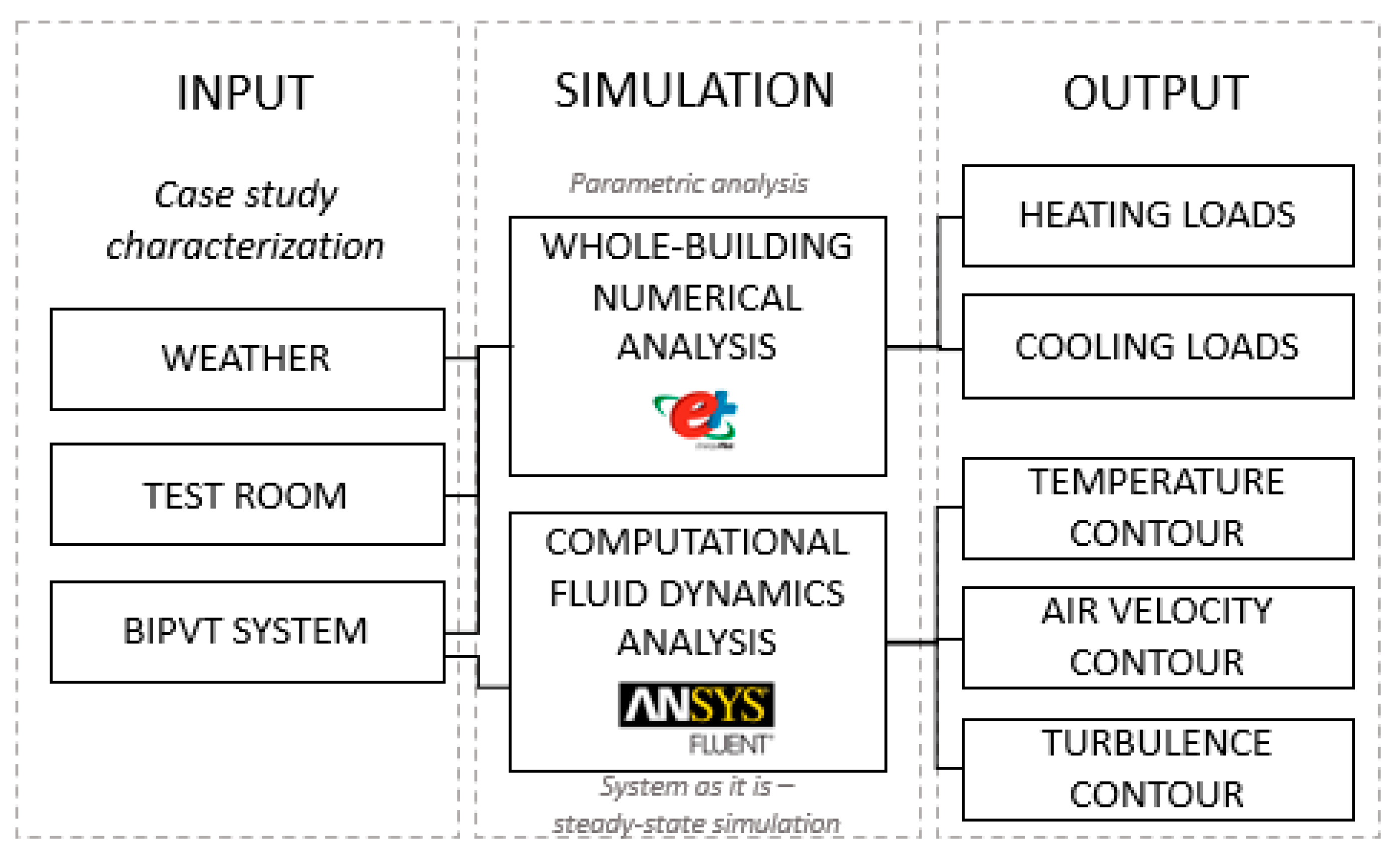
The methodology used to develop this work is based on: (i) case study characterization (presented in Section 3 in order to provide detailed description), with a special focus on the BIPVT system and the thermal zone in which it is inserted; (ii) whole-building numerical simulation; and (iii) CFD numerical simulation. This approach to evaluating the thermal performance is useful not only to NZEBs but to regular buildings as well. The approach is scalable in terms of adding multiple thermal zones (which is not the specific case of this work, that approaches only the pertinent thermal zone to the BIPVT system), and also in the scale of energy analysis, being possible to add various inputs and outputs to the simulation. Concerning the CFD system, it is also possible to scalate the methodology to other types of buildings and systems, and also vary from two-dimension simulation to three-dimension simulation and from steady-state analysis to transient analysis.
As a brief introduction to the case study, the test room is located in the Solar XXI building from the National Laboratory for Energy and Geology (LNEG). This building was designed as a low-energy-demand building that integrates renewable energy into the main façade and roof. The building integrates solutions and strategies aiming to reduce cooling loads using passive approaches and solutions, namely external solar shading, natural ventilation and passive cooling utilizing 32 buried pipes that exchange heat in the soil. The buried pipe system will not be further described in this work because it was not used during the entire testing period of the test room. For the heating period, the solution and strategies integrated into the Solar XXI building are the optimized envelopes externally insulated and the use of direct solar gain through the south-oriented main façade of the building. More details about the building may be found in [22].
Moreover, the main façade is composed by BIPVT systems that aim not only to generate electrical energy but also act as a natural heat recovery system. These systems are integrated into the main façade and consist of 76 photovoltaic multi-crystalline silicon modules with an area of 96 m2 and a 12 kW peak power. The average productivity is 1004 kWh/kW. The geometry and functionality of the BIPVT system will be further described in the next subsections. The system and test room will be further described in Section 3.
Figure 1 presents a flowchart with the schematic outline of the methodology used in the scope of this work.

Figure 1.
Methodology outline.
The numerical analysis was performed in this study both specifically for the BIPVT system and for the integration of the BIPVT system into the test room façade. The numerical analysis was structured in three parts. The first part described and characterized the case study. The second part developed the whole-building dynamic simulation employing a parametric analysis. The third part developed the CFD simulation.
This study adopted a methodology concerning building energy simulations in accordance with the work of [23,24]. For both numerical approaches (the whole-building dynamic simulation and CFD analysis), the case study was described concerning the BIPVT system and its boundary conditions. This section does not aim to extensively describe the numerical equations that support the computational modelling, as they are widely known and described in the literature, and may be found in [25], but instead to describe the parameters used for the simulation process and validation of the models.
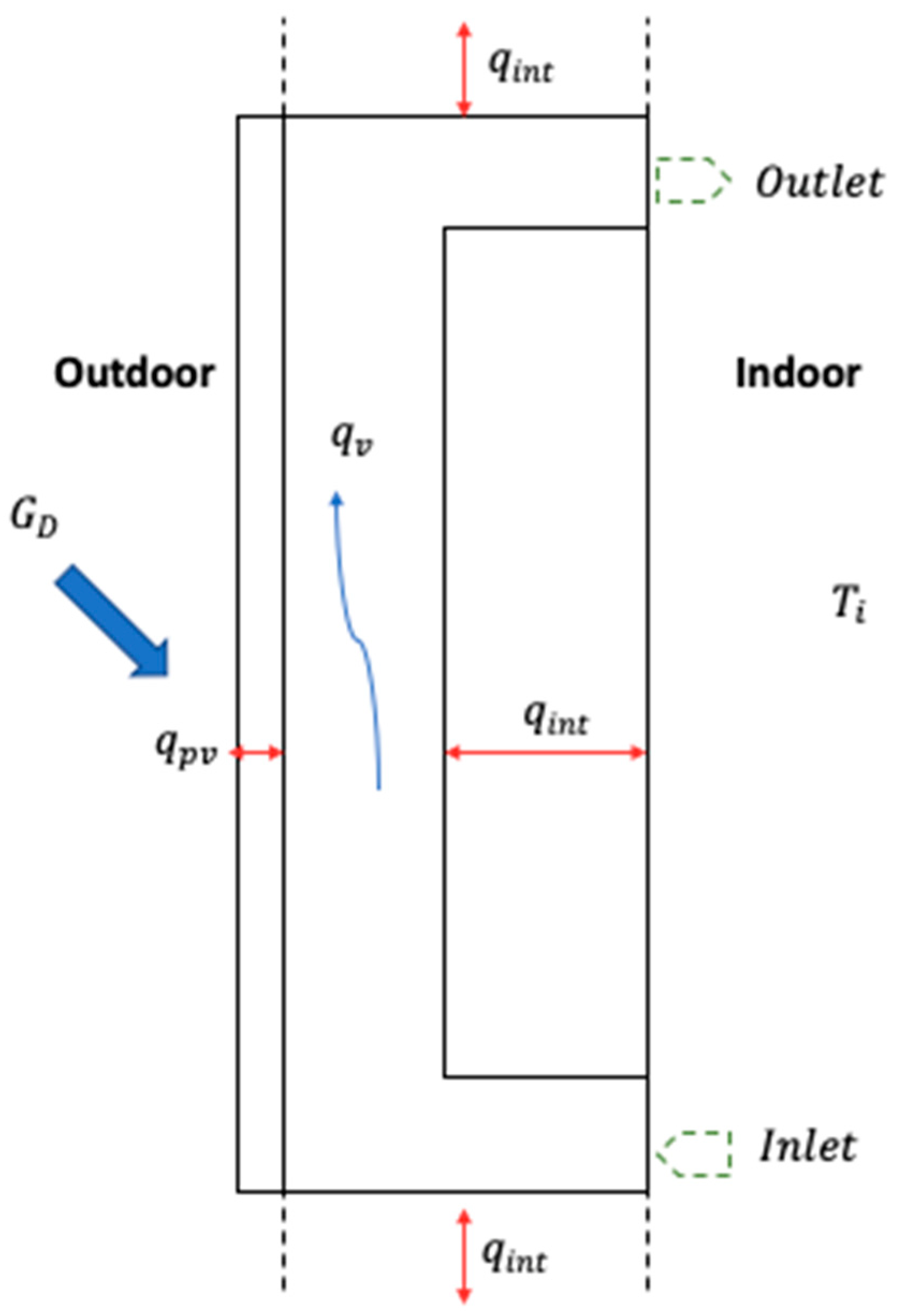
The heat balance of the BIPVT system is presented in Figure 2. It considers the solar gains and conductive and convective heat fluxes throughout the module. The heat transfer through radiation within the system was ignored in this scheme. In this scheme, qint stands for heat flux through the interior elements, qpv for heat flux through the photovoltaic module, qv for convective heat flux and GD for direct solar radiation.
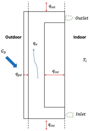
Figure 2.
Thermal balance scheme.
2.1. BIPVT Control Logic
The control strategies fundamentally contribute to achieving the NZEB concept. Among the different objectives of the control strategies, some of the most important are the comfort of the occupants and the efficiency of energy use while reducing the energy demand of a building. The control of the systems also has the potential to contribute to demand response strategies, as in [12]. The smart scheduling of the operation of the systems is important not only in scenarios in which model predictive controls are employed to reduce energy use in the building itself, as in [12,26], but also in a more general context in which the actions of the building systems are a part of the grid energy flux planning.
In its current state, the BIPVT system installed in the test room is manually operated. With the aim of improving the operation of the system, which can be subjected to occupants’ perception of the environment and also the availability for operation, the current study aims to assess the control logic throughout the parametric analysis of different setpoints for the BIPVT vents opening and closing. The proposed EMS control logic assessment for the automation of the BIPVT system does not account for the energy consumed to its own operation. Indeed, its focus is the reduction of the energy needs of cooling and heating of the adjacent thermal zone (the test room).
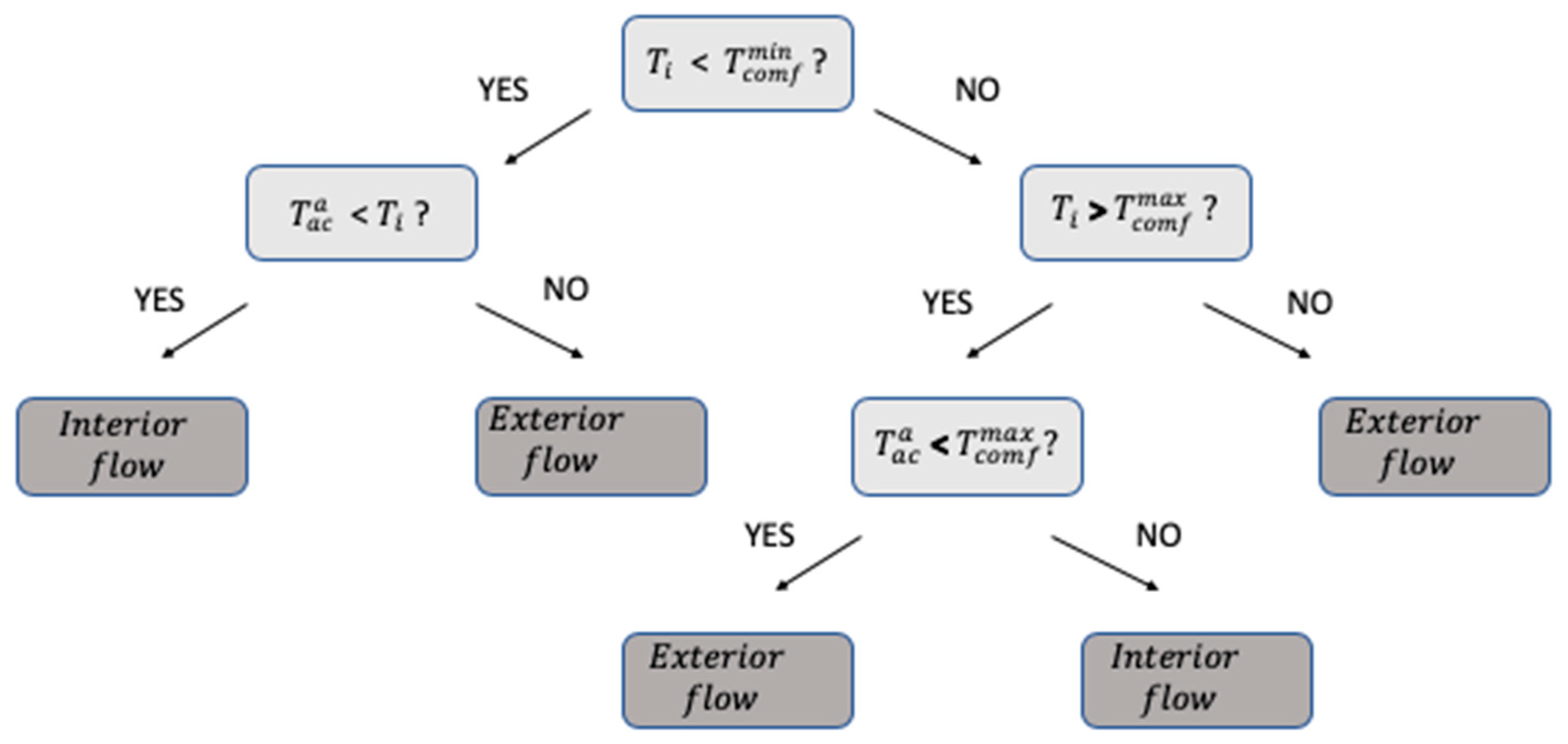
The proposed control logic process for the automatic operation scheme is presented in Figure 3. It takes into consideration: the maximum temperature of comfort () and the minimum temperature of comfort () between which the occupant is considered comfortable (comfort range temperature (); the indoor temperature (); and the air cavity temperature (). The temperatures considered for the operation may be changed according to the occupants’ preferences, in terms of setpoint definition for the smart operation of the system. However, during the development of this work, the range was assumed to be between 18 °C () and 25 °C (). The average temperature of the air cavity temperature () also interfered with the operation of the vents, as it is possible to see in the scheme. It is important to highlight here that the temperatures considered for the air cavity considering the obtained experimental values refer to a punctual value translating the temperature in the sensor’s location, whereas the average temperature accounts for all the sensors located within the air cavity (vertical duct, inlet and outlet).
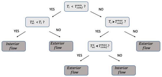
Figure 3.
Control logic for the automation process of the BIPVT system.
2.2. Whole-Building Dynamic Energy Simulations
Most studies on building heating and cooling load calculations are strongly based on computer simulations, due to the challenges posed by the many aspects involved in modelling the entire building. To evaluate the interaction between the system and the room, EnergyPlus software [27] was used (version 8.6.0.) with the primary purpose of estimating thermal changes, lighting levels, heating and cooling, natural ventilation, water uses, photovoltaic systems, thermal comfort indices, and other variables. It can be adapted to different climates from weather archives with hourly data. As a result, a wide range of calculated data, such as interior temperatures, surface temperatures, heat flow through building components, interior heat gains, air exchange, energy use and others, are obtained.
The real conditions dynamic simulation is focused on the Solar XXI NZEB test room and energy systems tested as integrated façade solutions. Overall, the main façade is south oriented, as was demonstrated in the case study section. The time step set for the simulation was 20-time steps per hours, beginning on 1 January and ending on 31 December, accounting for 8760 h simulated for each case in same boundary conditions regarding weather conditions for the parametric analysis (based on the original weather file for Lisbon) and a modified weather file for the model under validation process. The daylight saving period was set from 30 March to 30 October. The HVAC template used for nominal energy needs calculation was 20 °C for the constant heating setpoint and 25 °C for the constant cooling setpoint, and the results were obtained through the utilization of an ideal loads system.
First, the model for experimental validation was developed (M1). The M1 was elaborated to compare its results with the data recorded by the experimental campaign carried out at the test room site to validate the inputs inserted in the program. To ensure that the results obtained by computer modelling effectively represent the thermal behavior of the building, it was essential that the simulation model was calibrated correctly [28]. The model was validated as given by [29,30] for the performance criteria of the model validation. The usage pattern (occupancy, lighting and equipment) registered in the building for the considered days was inserted into the validation model. Moreover, observational measurements were taken to confirm the infiltration calculations. The temperature sensor used (series PT100) had a sampling interval of 1 min, and 60-min averages were calculated once the output of the simulation had hourly sampling. The sensor was located in the middle of the room, avoiding direct solar gains. Table 1 presents the sensors’ specifications.
The weather file containing the Test Reference Year (TRY) values of the city of Lisbon was modified, with radiation, temperature data and relative humidity recorded by the experimental campaign. The modification of the weather file may be a tricky process, and the steps follow the approach described in detail in [31]. The weather file was modified using the experimental data from January and February of 2018, and the remainder of the file was kept as the original. After the modification of the weather file, this study followed the simulation of the validation model.

Table 1.
Sensor specifications.
Table 1.
Sensor specifications.
| Observable Variable | Sensor Brand/Model | Range | Accuracy |
|---|---|---|---|
| Room temperature | Omega/PT100 [32] | −70 to 500 °C | 0.03–0.07 |
| Outdoor temperature | Omega/PT100 [32] | −70 to 500 °C | |
| Global horizontal radiation | Kipp & Zonen CM6B 951765 [33] | 200 to 4000 nm | <0.2% |
| Direct normal radiation (weather station) | Kipp & Zonen CHP1 100434 [34] | 200 to 4000 nm | <0.2% |
| Direct normal radiation (wall of test room) | Kipp & Zonen CHP1 100434 [34] | 200 to 4000 nm | <0.2% |
| Diffuse horizontal radiation | Kipp & Zonen CM6B 983431 [33] | 200 to 4000 nm | <0.2% |
| Air infiltration | Testo 425 | 0 m/s to 20 m/s | 0.01 m/s |
| Air cavity temperature | Omega/PT100 [32] | −70 to 500 °C | 0.03–0.07 |
| PV module temperature | Omega/PT100 [32] | −70 to 500 °C | 0.03–0.07 |
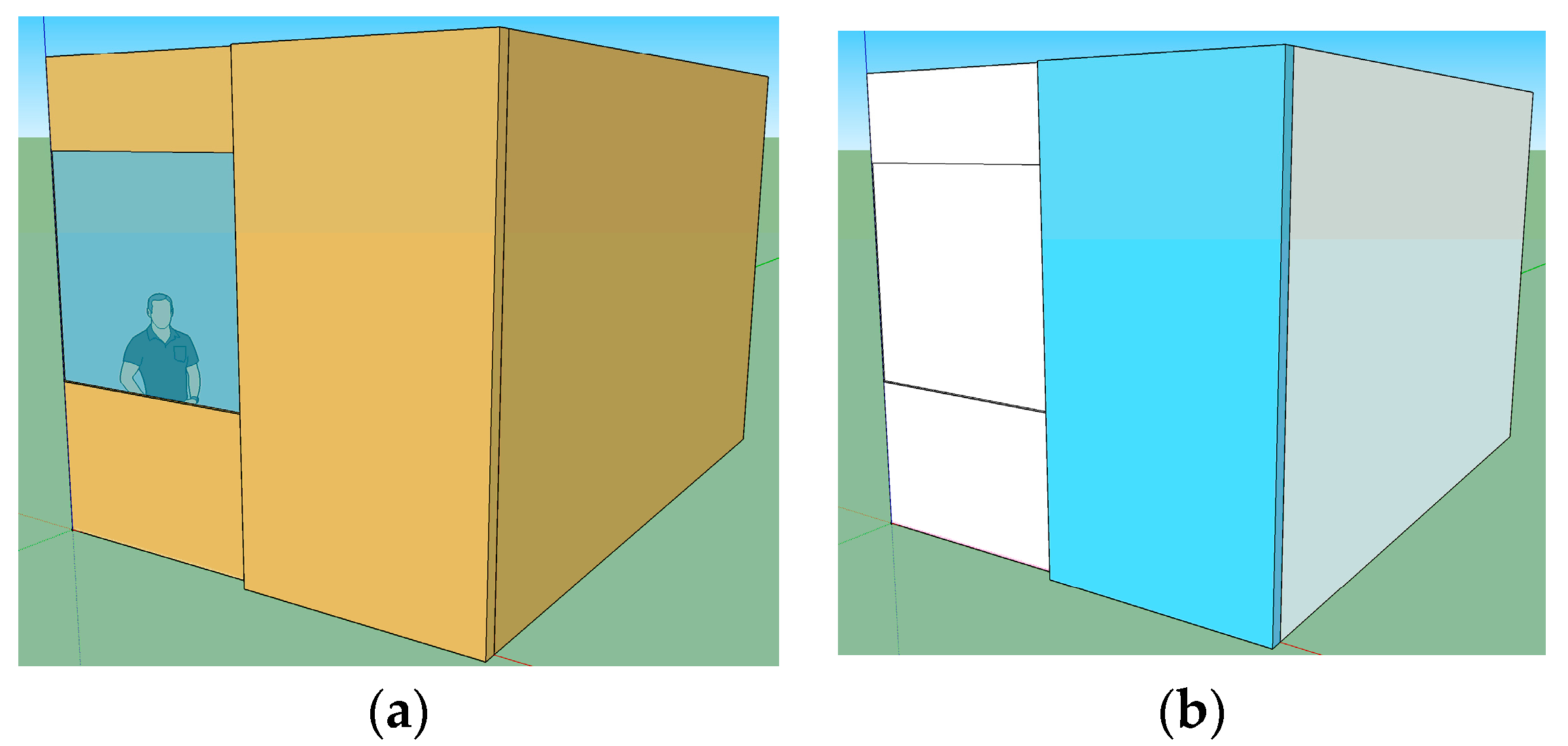
The simulation parameters used for the validation model are described in this sub-section and were kept for all the models developed in EnergyPlus in the scope of this work. The main simulation parameters and objects, and the value/option are described in Appendix A. The results obtained for the model using EnergyPlus software were compared with the temperature measurements made within the thermal zones in which the case study was performed. The root mean square error (RMSE) and mean bias error (MBE) were calculated and compared with the maximum allowable values for validation [28]. To achieve a more accurate validation of the model, two periods were used—from 22 January 2018 to 28 January 2018 and from 15 February 2018 to 22 February 2018—accounting for a total of 14 days. After validating the model, the parametric analysis proceeded. The parametric analysis accounts with different geometries for all the models. The geometries were developed, through the OpenStudio plug-in in SketchUp for the test room with the BIPVT element (Figure 4).
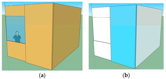
Figure 4.
Test room and BIPVT SketchUp geometry: (a) normal render, and (b) render based on thermal zones.
The parametric analysis aimed to recognize the impact of different parameters in the overall building performance. After validating the model (M1), the scenarios for the parametric analysis were set (M2 to M16), and the reference models were developed (M4). M4 was the model that effectively represented the building with the system as it is, considering geometry, air cavity thickness and air flow between zones obtained by experimental campaign. The reference model M4 was used for comparison with other models in which different strategies were inserted.
To simulate these models, all the inputs needed were added into the model on EnergyPlus and the weather file that contains the values of TRY (Test Reference Year weather data) of the city of Lisbon was used without any kind of modification (and thus different from what was previously used in the validation model).
A utilization pattern was also established for occupation and equipment for working hours from Monday to Friday, from 08:00 a.m. to 12:00 p.m. and from 13:00 a.m. to 17:00 p.m. Lighting was not considered in the simulations. When the blinds were completely opened, the daylight was sufficient to generate visual comfort of the occupants. The lighting system constituted a considerable internal thermal gain to the thermal zone—for comparative purposes, lighting was not considered as well in the set of scenarios in which the blinds were considered closed. It must be acknowledge, however, that as a real condition lighting may be needed in a situation where blinds are closed to achieve visual comfort for the occupants.
The total thermal gains were convective, radiant and latent gain in various proportions. Convective gains are instantaneous additions of heat to the thermal zone since the radiant gains are distributed on the surfaces of the zones where they are first absorbed and then released. Latent gains, in turn, need to be handled through ventilation and air conditioning [27].
The established BIPVT system infiltration of 0.01 m3/s and in the room 1.32 air change per hour were considered as constants during the simulation period. It is important to highlight that the BIPVT system was equipped with vents that increase the airflow of the natural convection through forced convection, and, despite not being tested in the experimental campaign, they were considered in the numerical analysis through the assumption of different airflow rates. The windows were closed all the time.
The scenarios simulated in the parametric analysis have been studied in terms of five groups of parameters:
- Window blind position (open or closed);
- Air gap thickness (0.5, 0.1, 0.16, 0.20 m);
- Zone mixing airflow (0.01, 0.02, 0.03 m3/s);
- Number of PV panels (4, 3, 2, 1 panel);
- Zone mixing setpoint for operation.
Table 2 presents the scenarios with the blinds open (except M2, that is presented as an exceptional comparison in the table because it corresponds to the BIPVT system without ventilation/air changes with the interior test room and with closed blinds) and accounts for 15 scenarios (14 with the blinds open and 1 with the blinds closed). The scenarios in Table 2 are also simulated with the blinds closed. While M2 corresponds to the model with the blinds closed and without ventilation/air changes with the interior test room, M3 correspond to the same configuration with the blinds open. For the BIPVT, M4 (the reference case, as previously explained) corresponds to the M1 (validation model) geometry configuration, but simulated for the whole year and with fixed parameters of ventilation between BIPVT air cavity and test room, whereas M1 was simulated in a free-floating mode for the validation period only (January and February) and no results for energy needs for cooling and heating are presented. Model 4 is represented by an air cavity thickness of 0.16 m, with a zone mixing airflow of 0.01 m3/s, four PV modules, and a fixed zone mixing scheduled from December to February.

Table 2.
Parametric analysis scenarios.
2.3. CFD Simulation
Following the whole-building dynamic simulation analysis, an additional brief assessment was completed using computational fluid dynamics (CFD) analysis. The numerical characterization of the façade elements was developed using the CFD approach through the use of the software Ansys Fluent [35]. It aimed to characterize the thermal behavior of the system in its fluid and solid parts through the analysis of temperature profile, air velocity and turbulence, taking into consideration the cross-section of the element in a bidimensional analysis. Although all three heat transfer modes were present in or around the multielement façade systems which form the object of the present study, this work will place emphasis namely on the conductive and convective heat transfer mechanism.
The equations that govern the fluid flow and heat transfer processes inside the air gap formed between the vertical façade solid elements are the equations of mass, momentum and energy conservation [36]. The fundamentals of the CFD technique are widely discussed in the literature and will not be further described here, besides the basics concerning the simulation set-up used. However, a detailed description of the computational fluid dynamics method may be found in [37]. For this kind of calculation, it is critical to select appropriate boundary conditions that best represent the system.
The general scheme of analysis is briefly explained here. It began by designing the systems’ geometry using the Ansys Design Modeler according to the data provided in the case study description. The next step was to determine the mesh to be used in the fluid and solid parts, followed by the setup of the simulation. The setup of the simulation was done through the consideration of general features (as equations, steady-state mode, among others), model definition, the boundary conditions of the system, reference values, the solution, and initialization configurations. In the solution tab, it was possible to set the methods and monitors to be displayed, the variables to be calculated, and the reporting variables. The model results were observed through the selected plots and graphs.
The thermal behavior of the system was studied in a steady-state simulation. The simulation setup is briefly described here. The turbulent motion, described by the Navier–Stokes equations and characterized as an irregular condition of the flow with random variation with time and space coordinates, has been considered using the k-ε model with standard wall functions. These equations are solved by the use of the Semi-Implicit Method for Pressure-Linked Equations (SIMPLE) algorithm, and are essentially a guess-and-correct procedure for the calculation of pressure on the staggered grid arrangement introduced above. The method is illustrated by considering the two-dimensional laminar steady flow equations in Cartesian coordinates.
The energy model was considered activated. The turbulent viscosity was computed by combining k and ε, while the constants assumed the default values of C1ε = 1.44, C2ε = 1.92, C3ε = 0.09, σk = 1.0, and σε = 1.3. The standard k-ε model was used to perform the calculations in the software. The simplest “complete models’’ of turbulence are the two-equation models in which the solution of two separate transport equations allows the turbulent velocity and length scales to be independently determined. The pressure–velocity coupling used the coupled mode, whereas the influence of buoyancy force caused by the different densities due to the heating process was considered by inducting the Boussinesq approximation model (Boussinesq hypowork). This method uses a starting guess for pressure and velocity to solve the corresponding velocities via momentum equations, followed by introduced correction factors until convergence [37].
The standard k-ε model is a semi-empirical model based on model transport equations for the turbulence kinetic energy (k) and its dissipation rate (ε). The model transport equation for k was derived from the exact equation. In contrast, the model transport equation for ε was obtained using physical reasoning and bears little resemblance to its mathematical counterpart, according to the software theory guide. The Boussinesq approximation was based on the assumption that the components of the Re stress tensor are proportional to the mean velocity gradients, assuming that eddies behave like molecules, that turbulence is isotropic, and that there exists local equilibrium between stress and strain.
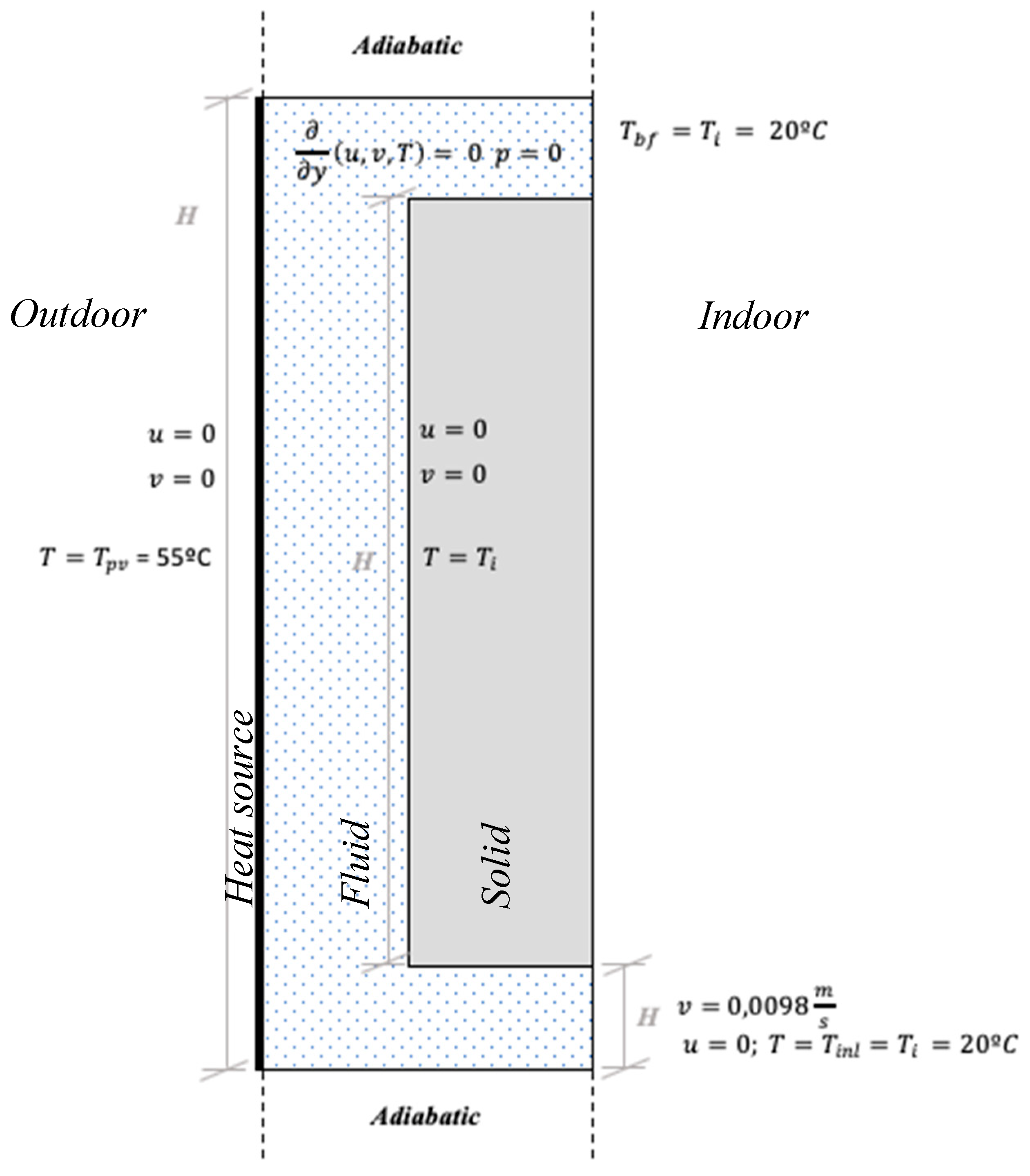
Thus, default residuals were used for continuity, x-momentum, y-momentum, energy, turbulence kinetic energy and the turbulence kinetic energy dissipation rate for checking the convergence of the solution. The more detailed numerical formulation may be found in the software theory reference guide. Figure 5 presents the boundary conditions and the domains of the system.
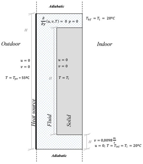
Figure 5.
Boundary conditions and domains in the computational fluid dynamics (CFD) analysis.
All CFD problems are defined in terms of initial and boundary conditions, as has been deeply explored in [37]. Flows inside a CFD solution domain are driven by the boundary conditions, and the most common cause of the rapid divergence of CFD simulations is an inappropriate selection of boundary conditions. It is essential that the user specifies these correctly and understands their role in the numerical algorithm. In transient problems the initial values of all the flow variables need to be specified at all solution points in the flow domain. However, this work assumed steady-state conditions. The boundary conditions considered in the scope of the CFD simulation of this work were the inlet, outlet, solid surfaces and prescribed pressure. The most accurate simulations can only be achieved by supplying the measured inlet values of turbulent kinetic energy k and dissipation rate ε. However, in most cases, such data were often not available, and default values were adopted.
In this CFD analysis, the PV module was considered to be a heat source surface for all the BIPVT systems, with an associated temperature. The temperatures assumed for the PV surface () at a given moment (steady-state condition) were based on the experimental campaign previously developed, as well as the interior module/wall temperature. The interior wall of the BIPVT system was assumed to have the same temperature as the room ( at the initial boundary condition. The inlet velocity was considered as the value registered in the experimental campaign for the system (instant observation through the use of a non-fixed anemometer), corresponding to 0.0098 m/s normal to the boundary. The inlet turbulent intensity fraction was 0.5, and the turbulent viscosity ratio was 10. The outlet had a backflow direction specification method as normal to the boundary, while the backflow pressure specification was the total pressure. Moreover, the was assumed to be the same as the at a given moment.
All the elements were simulated under the same conditions of the heat source and inlet velocity to obtain comparable values. This was contrary to the experimental campaign in which each one of the elements was evaluated at a different time period with different boundary conditions. The PV surface was considered at 55 °C (based on the experimental data for the particular day of the BIPVT system). The was also the same as the experimental campaign for the given day. The outlet boundary conditions may be used in conjunction with the inlet boundary conditions. The air properties were sourced from the software database. The water properties were also sourced from the software database. The solid properties were mentioned in the case study description, and no-slip and no-permeability hydrodynamic condition along X and Y directions were considered.
It is essential to highlight that the real system temperature presented more heat losses, since in the CFD simulation the upper and bottom surface of the air cavity were considered adiabatic due to the lack of control in the experimental campaign to determine the heat fluxes through these surfaces. By simplification, the mesh was considered uniform for all the models. Considering these remarks, the results obtained for each simulation are presented in the following section.
3. Case Study Description
3.1. Location and Weather
The case study was located in Lisbon, Portugal in the Solar XXI building (38°46′21.74″ N; 9°10′35.54″ W) of the National Laboratory for Energy and Geology. In [38], it is described that the continental Portuguese territory (between latitudes 37° and 42° N) is located in the transitional region between the subtropical anticyclone and the subpolar depression zones. Lisbon has a subtropical Mediterranean climate and, according to the Köppen climate classification, is classified as Csa [19,20,21] with the Atlantic Ocean wind influencing the rain but maintaining moderate temperatures. The climate is also influenced by the orography and the effect of the Atlantic Ocean, with the continental climate affecting around 220 km of the regions furthest from the ocean.
3.2. Test Room Characterization
The physical characteristics of the building in the scope of this research are composed by the description of the envelope of the test room (the exterior and interior walls, floor, ceiling, roof and fenestration surfaces) considering the thermal characteristics of the elements. Also, other parameters such as internal gains and air infiltration are described. The output of this section will be the data to be used to describe the building in the numerical modelling assessment.
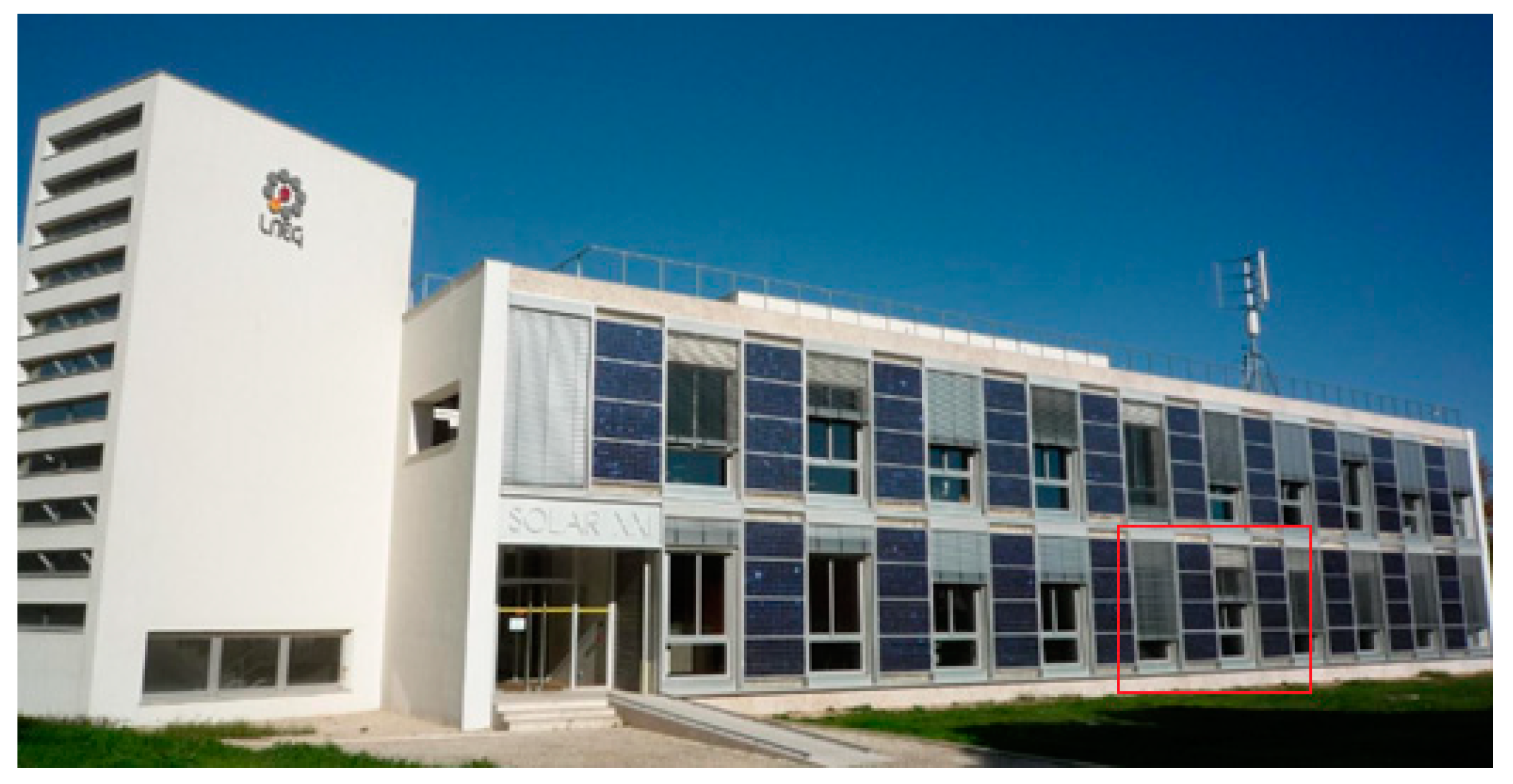
Two test rooms were used in the Solar XXI building to test building-integrated solar energy systems and energy flexibility, the intelligent management of system-to-building interaction, and occupant behavior. In Figure 6, a red rectangle signals the location of the test rooms in the main façade. In the present work, only one of the test rooms (NZEB_LAB 1) was object of study, since this is the one where a complex system of automation and monitoring has been implemented.

Figure 6.
The Solar XXI building and the location of monitored test rooms (within the red rectangle).
The geometry and picture of the test rooms are shown in Figure 7: Figure 7a presents a cross-section view and Figure 7b presents an indoor picture of the test room and BIPVT system. The test room under analysis in the present work has a floor area of 16.70 m2. The exterior wall has a gross area of 3.97 m2, with a glazing area of 2.82 m2. The lateral walls (West and East oriented) are adjacent to other rooms with similar thermal behavior. The interior wall that opposes the exterior wall (North oriented) is adjacent to the corridor of the building. All of the test room surfaces are subjected to heat losses and gains. However, the interior walls are in contact with thermal zones with similar thermal behavior; thus, the heat gains are not accentuated, and these surfaces are considered adiabatic during numerical analysis. The ceiling of the room is also adjacent to a thermal zone with similar thermal behavior. It was also considered adiabatic in the numerical analysis, as was the floor. There is also a floor underneath the test rooms. Specific details concerning the architectural elements and their thermal characteristics may be found in Appendix B (Table A1).
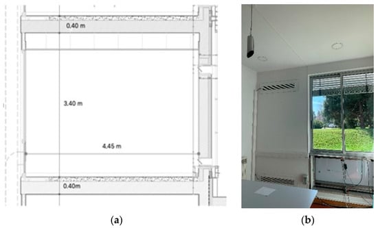
Figure 7.
Test room: (a) cross-section view; (b) indoor picture and Building Integrated Photovoltaic Thermal (BIPVT) system.
According to [39], the thermal zones are the space or set of spaces that can be considered together due to their similarities in terms of user profile, lighting and equipment, mechanical ventilation and air conditioning system, and air-conditioned spaces. Due to the similarities in terms of solar exposure conditions, small commercial buildings and services with a useful floor area of up to 250 m2 can be considered to have only one thermal zone, according to [39]. However, in the scope of this study, the test room was considered as a thermal zone to obtain accurate and detailed results on the building energy simulations considering the test of the BIPVT system (further described in the next sections). The concept of the thermal zone introduces the boundary conditions, envelope and internal gains assumed for further modelling and simulation. The building’s thermal behavior and the related energy use are defined by a complex interaction of heat gains, losses and storage in building materials and finishing.
The solar radiation transmitted through the transparent components of the building skin, such as windows and skylights, originate a significant heat flux source and direct heat gains. Another main contributor to the heat balance of a building is the heat flow through the opaque building envelope. These transmission losses or gains can mainly be described by the physical process of heat transfer through the materials. These fundamental principles will not be further described as they are common knowledge in the field. However, further details may be found in [40]. Also, [41] describes further the main components of heat fluxes in buildings.
The accurate description of the building envelope and the previously presented specific climatic conditions were crucial for the success of the energy analysis. As described by [41], many of the boundary conditions inducing these heat fluxes are not constant over time. Weather conditions, such as outside air temperature and solar irradiation, are continually fluctuating. In most cases, the building operation also imposes fluctuating interior heat loads. While solar radiation and convective heat flows vary nearly simultaneously with the fluctuation of the outdoor boundary conditions, the conductive heat flows through the building skin will present a time lag compared to the external excitation.
A significant heat flux consists of heat generated (internal gains) or extracted interiorly due to building operations. These thermal loads stem from heat losses from various sources such as artificial lighting, office equipment and metabolic heat gains from building occupants. The internal gains through lighting, occupation and various equipment are often significant elements in the thermal balance of the zones. The gains regarding the total convective heat are the result of radiant and latent gains in various proportions.
The occupancy component is described not only based on the number of occupants but also based on the usual metabolic rate for the performed activities (activity levels), the radiant fraction, and the comfort level expectations according to the season. The internal gains related to the devices and lighting inside the test rooms are described in terms of the maximum level of design, and the latent, radiant and lost fractions. The heat gains from lighting in particular may be broken down between the visible portion and the thermal portion [27]. The use of scheduling described by a fraction of peak usage for each time interval details on the occupant behavior for whole-building energy simulations may be found in [42].
The output of this section will be the data to be used to describe the internal gains of the building in the numerical modelling process. Appendix B (Table A2, Table A3 and Table A4) also presents details concerning the internal gains of the building due to occupation, lighting and equipment, respectively.
Finally, ventilation and infiltration through the building façade will be responsible for other components of the heat flux process in buildings. In any case, determining the real air infiltration in a room is a complicated process, because any gap present in the envelope can be an inlet or outlet of the air, and the air infiltration can have different values in each segment of the gap area. The air movement, however, will be punctually determined through the experimental campaign in the next section.
3.3. BIPVT Characterization
The BIPVT systems with heat recovery aim to increase the outlet temperature compared to the inlet temperature of the system, having as source air the air volume from the test room. They are composed of a PV area per BIPVT system of 5.25 m2 (four modules), with vent opening areas (inlet at the bottom and outlet at the top of the system) of 0.186 m2 each for the interior and another two with the same area for the exterior (allowing circulation between air cavity and the exterior to cool the PV panels). Between the interior wall and the PV modules, there is an air cavity of 0.16 m of thickness. Moreover, it is important to mention the properties of the air considered to be flowing or stationary in the air cavity. It is considered to have a density (ρ) of 1.213 kg/m3, a specific heat of 1006.7 J/kg.K, a thermal conductivity of 0.02544 W/(m.K) and viscosity of 1.79 × 10⁻⁵ kg/m.s. [35]. Table 3 presents the thermal characteristics [16] of the constructive elements of the BIPVT systems, the “exterior wall” that separates the test room from the air cavity between wall and photovoltaic panels.

Table 3.
Characteristics of the BIPVT constructive elements.
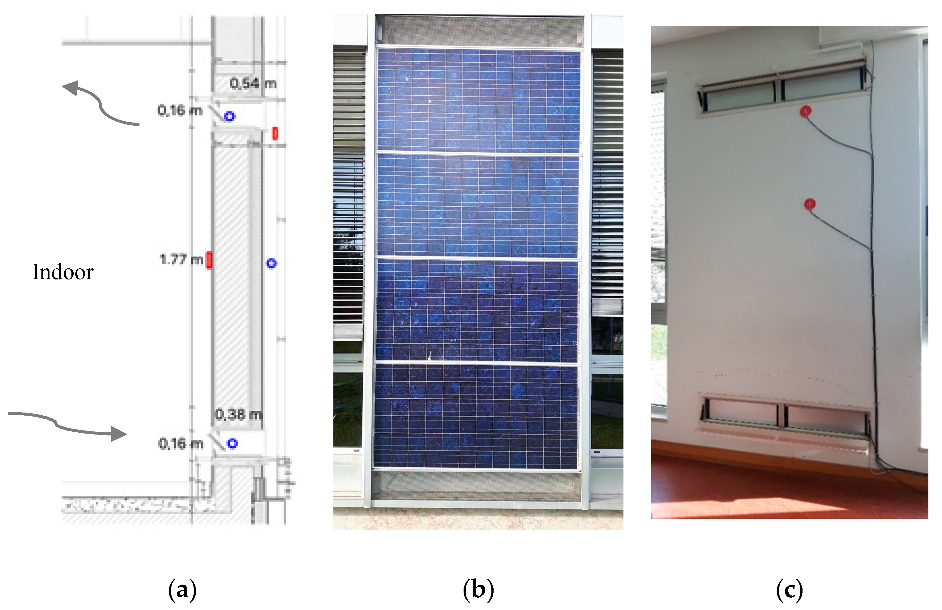
Figure 8 presents the details of the geometry of the BIPVT systems as well as the pictures of the exterior and interior view of the system. The BIPVT thermal behavior is registered by temperature and heat flux sensors. There is a total of three temperature sensors located at the bottom (inlet), at the middle of the air cavity and at the top (outlet). The temperature sensor locations are signaled with blue circles, whereas the heat flux sensors are signaled with a red square. The temperature sensors located in the inlet and outlet openings are located 0.08 m from the interior surface of the opening. The heat flux sensor used in the scope of the work is the one located in the wall, and its height is approximately 0.88 m above the inlet opening, in the same height as the air cavity temperature sensor. The dimensions of the air duct are also shown in the picture.
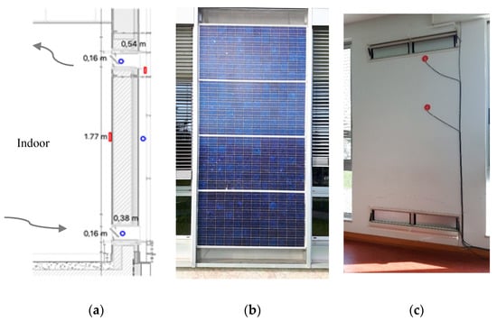
Figure 8.
(a) Cross-section of the BIPVT system and sensors location; (b) exterior view of the system; (c) interior view of the system.
The BIPVT system is composed by four vents (one at the bottom and one at the top at the indoor component and outdoor component), as was previously described, that allow either interior circulation to heat the room or external circulation to cool the PV panels. The vents are operated either manually according to the occupants’ wishes or automatically, according to a control logic for the automation process. The manual operation was segmented in two: heating mode and cooling mode. The heating mode refers to wintertime: at night all the vents are closed, and during the day the interior vents are opened. The cooling mode refers to summertime, in which the interior vents are closed and exterior vents are opened both during night and day.
4. Results and Discussion
Following the methodology section, in which the case study characterization was outlined and the simulation processes determined, this section presents the obtained results.
4.1. Whole-Building Dynamic Simulation Results
4.1.1. Model Validation
The results obtained for the model validation (M1) are shown in Table 4 for the first period (22 January 2018 to 28 January 2018) and in Table 5 for the second period (15 February 2018 to 22 February 2018) accounting for a 14-day validation period. The limits for validation concerning the Coefficient of Variation of Root-Mean Squared Error (cv(RMSE)) and the Mean Bias Error (MBE) are 0.3 and 0.1, respectively. Given the obtained results, the model was considered validated.

Table 4.
Validation of the model for the period 22 January 2018 to 28 January 2018.

Table 5.
Validation of the model for the period 15 February 2018 to 22 February 2018.
4.1.2. Parametric Analysis
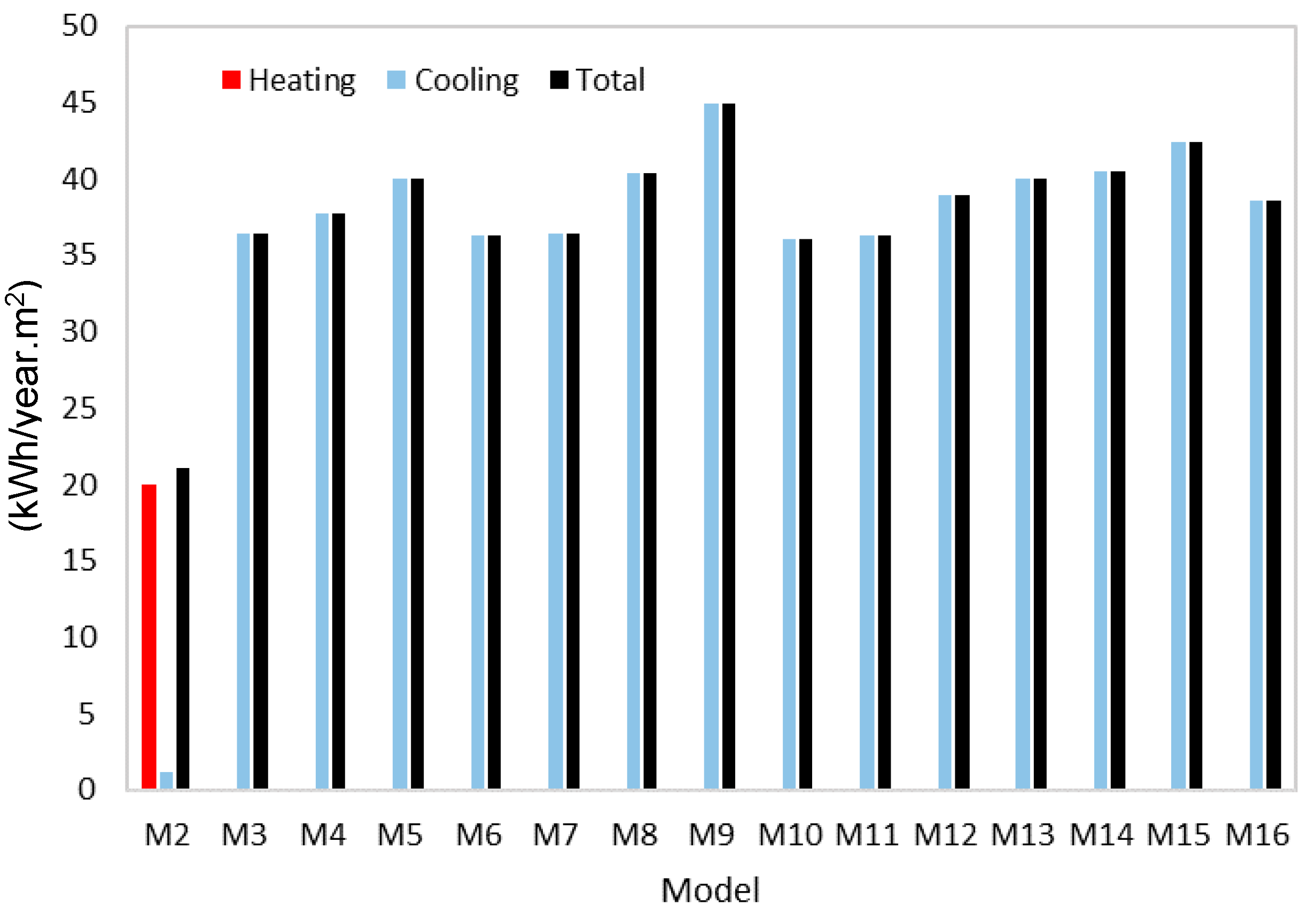
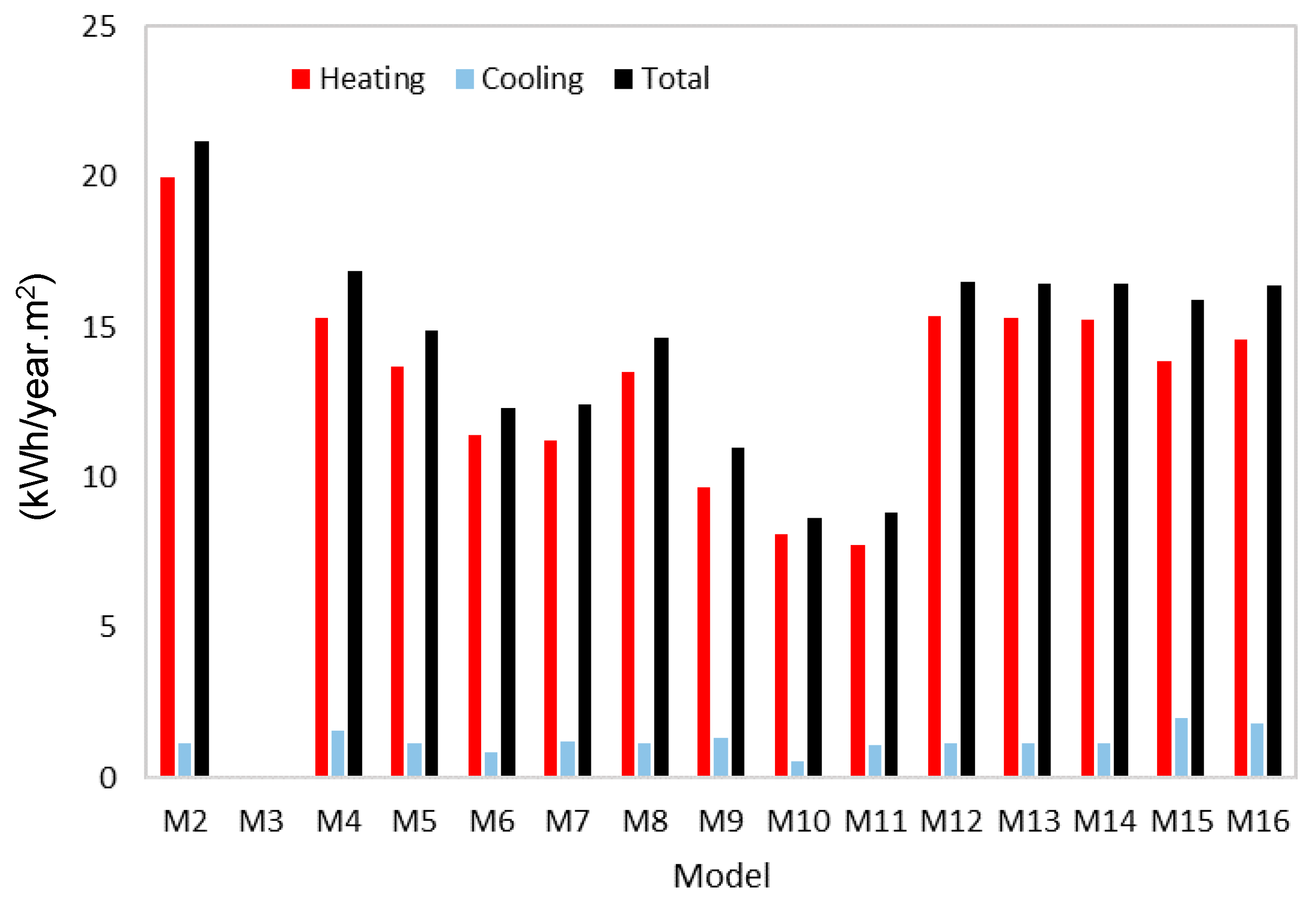
The obtained results are fully presented here in terms of the nominal energy needs for the heating and cooling of the building, taking into consideration a setpoint of with a lower limit at = 18 °C (under which the building will be thermally conditioned) and the upper limit at = 25 °C (above which the building will be thermally conditioned). Table 6 presents the results for all the scenarios under consideration in this parametric analysis, while Figure 9 and Figure 10 graphically display the results.

Table 6.
The whole-building dynamic energy needs simulation results (in kWh/m2/year) and percentage variation (%) of total energy needs in relation to the M4 reference scenario.
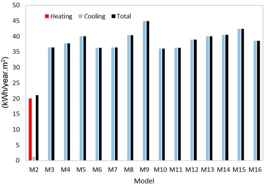
Figure 9.
BIPVT simulation results for the energy needs with the window blinds always open (except M2 which is M3 closed, for comparison purposes).
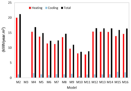
Figure 10.
BIPVT simulation results for the energy needs with the window blinds always closed (in this case, M3 = M2).
To evaluate the impact of the strategies for energy use while reducing the uncertainty brought by the direct heat gain through the window, two sets of scenarios were simulated. In the first set, the blinds were considered open all the time, with exception of the M2 that was inserted in the graph (Figure 8) for the sake of comparison. In the second set (Figure 9), the blinds were considered closed all year. In the second set M3 is equal to M2, which is the reason why no results are shown for this model. It is possible to see that the cooling energy needs are predominant and may constitute the total energy needs for the building to reach comfortable temperatures.
It is possible to see that there is a shift in the energy needs, from cooling to heating, showing the huge role the direct heat gains play in the thermal behavior of the building. In most cases, the total energy needs dropped by almost half of their value. The models grew in complexity, and for this reason M2 shows the results for the room with the windows closed and without any air mixing between the zones, while M3 shows the results for the room with the windows opened and no air mixing between the zones. From M4 onwards, the models begin to present air mixing between zones.
From model 3 to model 16, the simulations concern the use of the BIPVT element. Model 4 to model 7 present the room with the BIPVT with 0.16 m of air cavity thickness, varying the zone air mixing parameter from two fixed schedules of operation to two smart operations (0.01 m3/s). Among these models, the fixed operation schedule (presented in the simulation scenarios) resulted in higher values of the nominal energy needs. In contrast, the smart operation (with very similar results between them) present a decrease in the nominal energy needs, in comparison with a fixed schedule. From model 8 to model 11, the schedule of operation of the air mixing was also evaluated; however, with an increased flow of 0.02 m3/s. In this group, the smart operation schedule shows similar results to the previous ones with reduced airflow. However, the energy needs for the fixed schedule increased.
The system with the highest energy needs was M9 (0.02 m3/s in the zone mixing system and the setpoint of operation from November–March from 10 h to 16 h) and the variations among models reach 10 kWh/year·m2, not considering M2 which represents the system with the window blinds always closed. For most of the models, the results vary slightly. Considering the simulations with the blinds always closed, it is possible to notice, however, that M9 is one of the models with lower total energy needs.
Overall, as seen in the results, for the cases in which the room did not have the blind closed the BIPVT was the system with the highest number of scenarios in which the nominal energy needs increased compared to the reference model, reaching a percentage increase of nearly 20%. Still considering the blinds opened, for the best situation in each one of the systems, concerning the BIPVT system the model 6 and model 7 (smart operation of the air mixing between zones), model 10 and model 11 presented improvements in comparison to the reference model (the flow increased to 0.02 m3/s with smart operation).
When the simulation set is changed to avoid the direct solar gains through the use of a blind on the window, as was previously seen, the situation is inverse. In this situation of the avoidance of the direct solar gains, all the models contributed to reducing the energy needs compared to model M2, where only the BIPVT system existed. Still, no air change occurred between the room and the system. When the window blind was open, the smart operation of the air mixing was the main contributor to reducing the energy needs of the building, showing that a passive operation is not the best choice when comparing to an operation focusing on meeting temperature requirements. The airflow of the air mixing between the systems and the room does also have a positive impact for the BIPVT system, but may have a reverse effect on the BIPVT due to the bigger area of the heat source surface (four PV modules instead of one).
4.2. CFD Simulation Results
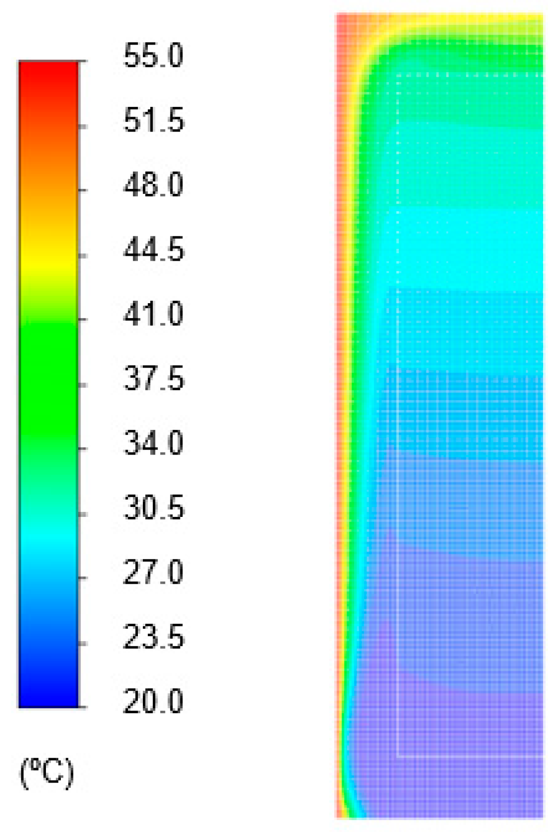
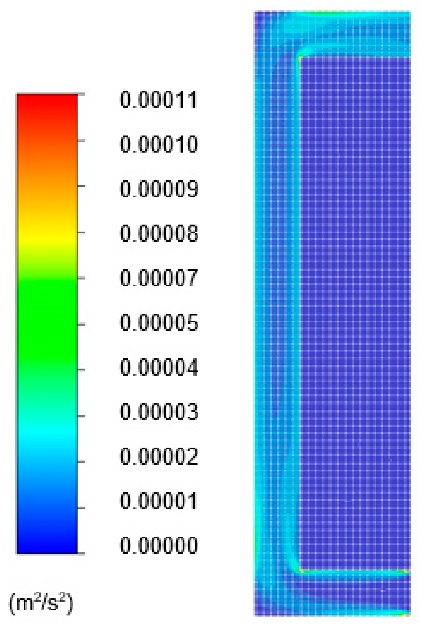
The BIPVT analysis used a mesh size of 0.005 m, chosen due to the computational capabilities to process the mesh given the area of the geometry, and the results are presented for temperature distribution in the air cavity and interior wall, velocity of air inside the cavity, and turbulence. The results for the temperature contour of the cross-section are presented in Figure 11. Figure 12 presents: (a) the velocity contour of the cross-section and (b) detail on the outlet vectors of velocity. Turbulence is presented in Figure 13.

Figure 11.
BIPVT temperature contour (°C).
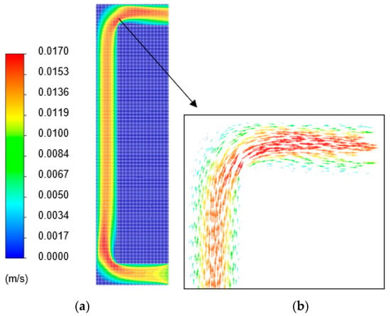
Figure 12.
BIPVT velocity contour (m/s).
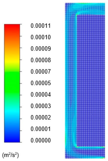
Figure 13.
BIPVT turbulence contour (m2/s2).
Considering the BIPVT system, the temperature increased due to the source of heat from the PV module entering the cavity in the inlet at a defined temperature of 20 °C and leaving the air cavity at a Tout of near 35 °C. The solid temperature presented a gradient that varies from 20 °C to 31 °C, similar to the air cavity, achieving higher temperatures in the upper part of its geometry. The temperature was higher near to the PV module surface, as this was the heat source for the simulation. The air cavity velocity reached a value to 0.017 m/s at some points, showing an increase of 0.007 m/s concerning the inlet velocity.
In the BIPVT case, there was only one sensor to represent the air cavity results in terms of air temperature. The position of the sensor (installed in a period prior to this study), impacted the results not only in vertical axis terms but also in the distance from the heat source surface (PV module) or the interior part of the system. Considering the middle height of the system, in horizontal axis terms, the temperature varied from 23 °C (near to the interior part surface) to 55 °C (value of the heat source surface temperature). The air velocity was also shown to have increased inside the air cavity due to the buoyancy effects of the natural convection.
The data was considered validated, employing temperature comparison with the experimental data concerning the detailed day of each BIPVT and BIPVT system. This analysis through the CFD software, even though was not extensive, was fundamental in different ways. First, the detailed profile of the cross-section modelling results was useful to understand the impacts of the sensor location on the results of the experimental analysis. For example, and taking into consideration the presented results from a sensor located in the lower part of the air cavity closer to the interior module, the results from a sensor located in the upper part of the air cavity closer to the PV module would result in a higher temperature gradient within the air duct, reflecting in a higher efficiency value than the actual efficiency of the system (keeping the other parameters constant).
This highlights the importance of the proper experimental setup disposition within the system to obtaining more accurate results. Moreover, it enhances the importance of having more than one sensor to characterize the temperature profile and, in experimental campaign terms, the air cavity.
However, it is important to refer to that the elements are dynamic in terms of heat transfer, and the CFD analysis performed in the scope of this work was a steady-state simulation representing the results of the calculation (until reaching convergence) for a particular set of inputs. In other words, this represented a specific hour of the day and room condition in terms of the Tinl, interior wall/module temperature and backflow in the outlet. For further representation during the year, the BIPVT systems should be tested with a CFD analysis for more than one condition, in different hours of the day, and preferably in different weather stations. The CFD analysis was also shown to be very useful in a preliminary analysis and the pre-manufacturing of the final BIPVT system design, to access the better materials and geometry more cost-effectively before production.
5. Conclusions
The numerical analysis was developed to evaluate the impact of the systems on the nominal energy needs of the adjacent thermal zone, namely for heating and cooling. The numerical analysis was segmented in two parts: (i) the dynamic simulation of the building in real condition through the use of the EnergyPlus, and (ii) component assessment through CFD analysis in a steady-state mode through the use of ANSYS Fluent. It was found that the energy needs of the test room can effectively be reduced by the use of the BIPVT elements, up to 48% in a scenario with an air cavity thickness of 0.16 m, a zone mixing airflow of 0.02 m3/s, 4 PV panels (the height of the system) and with smart controlled vents working on a whole year basis when the source temperature (air cavity air) is higher than 18 °C and the room temperature is lower than 24 °C. However, careful analysis must be completed concerning the configuration of the system in use—the operation mode, zone air mixing flow between zones, and also the thickness of the air cavity—due to the integration with other passive systems in the test room, as is the case of the window that allows direct solar gains. It was perceived that not all the configurations brought benefits to the test room in thermal terms. Some of the configurations raised the nominal energy needs and overheated the room, and they were mainly the ones with a fixed setpoint in the BIPVT system operation. Concerning the CFD analysis, it was possible to perceive an increase from 20 °C to 31 °C in the air cavity air temperature, supporting the suitability of the system for the application as a thermal heating recovery system.
The automated operation of the vents in the BIPVT system, enabling either exterior ventilation or interior ventilation, was the parameter with the highest impact on the reduction of the energy needs for cooling and heating. The obtained results showed that the increase of the airflow in the zone mixing could be beneficial in some cases, namely when coupled with smart operation. These results strongly highlight the importance of smart operation due to the automation in the BIPVT systems, in particular for mild climates like that of Portugal. In mild climates, the daily temperature in a thermal zone can range from below the minimum comfort temperature to above the maximum comfort temperature, contributing to increasing the thermal discomfort due to overheating or excessive cooling. In this scenario, the flexibility of the smart systems is fundamental to adapt to the different thermal conditions during the day and the different seasons of the year. Also, the occupants may be able to interact with the BIPVT systems human–machine interface (HMI) to set their preferred band of temperatures, as the thermal comfort preferences may change from one building user to another.
This work contributes to the advancement of the BIPVT in façades, and more specifically generates more detailed data of the behavior of these systems not only in the city in which the case study is located (Lisbon, Portugal) but also in other locations with similar climates.
Author Contributions
Conceptualization, K.B. and L.A.; methodology, K.B. and L.A.; software, K.B.; validation, K.B.; investigation, K.B., L.A., M.d.G.G. and C.S.S.; writing—original draft preparation, K.B.; writing—review and editing, L.A., M.d.G.G. and C.S.S.; supervision, L.A., M.d.G.G. and C.S.S.; project administration, L.A. All authors have read and agreed to the published version of the manuscript.
Funding
This research was funded by FCT/MCTES (PIDDAC) and European FEDER from Regional Operation Program of Lisbon, Refª. LISBOA-01-0145-FEDER-022075.
Acknowledgments
NZEB_LAB—Research Infrastructure on Integration of Solar Energy Systems in Buildings” (Refª. LISBOA-01-0145-FEDER-022075)” is financed of national funds FCT/MCTES (PIDDAC) and European FEDER from Regional Operation Program of Lisbon.
Conflicts of Interest
The authors declare no conflict of interest.
Appendix A
The EnergyPlus simulation parameters used in the scope of this work are:
- Simulation control: “run simulation for Weather file run periods”;
- Building: south oriented, solar exposed, wind exposed, city, convergence criteria for thermal loads of 0.04 and for temperature 0.40 °C, with solar distribution full interior and exterior, and 25 days of convergence;
- Shadow calculation: 20 days (standard value);
- Surface convection algorithm: inside and outside, DOE2 and TARP;
- Timestep: 20 timesteps per hour;
- Site location: Lisbon;
- Run period: whole year;
- Schedules compact: based on the previously described occupation pattern during a typical week of work;
- Surface elements: as previously described in the case study section;
- Surfaces and thermal zones: as previously described in the case study section;
- Interior loads: people, lights and equipment as previously described in the case study section;
- Infiltration flow rates: as previously described in the case study section;
- Output reporting: variable dictionary, variables (zone temperature and ideal loads) and diagnostics, with display of extra warnings.
Appendix B
This appendix presents the tables with data pertinent to case study description.

Table A1.
Characteristics of the test rooms envelope components.
Table A1.
Characteristics of the test rooms envelope components.
| Opaque Elements | Elements | Thickness (m) | Conductivity (W/(m·K)) | Density (kg/m3) | Specific Heat (J/(kg·K) |
|---|---|---|---|---|---|
| Exterior walls | Traditional plaster | 0.030 | 1.300 | 1900 | 1000 |
| EPS | 0.060 | 0.040 | 1000 | 1400 | |
| Masonry | 0.220 | 0.420 | 1000 | 790 | |
| Traditional plaster | 0.020 | 1.300 | 1900 | 1000 | |
| Interior walls | Traditional plaster | 0.010 | 1.300 | 1900 | 1000 |
| EPS | 0.060 | 0.040 | 1000 | 1400 | |
| Masonry | 0.110 | 0.410 | 1455 | 790 | |
| Traditional plaster | 0.010 | 1.300 | 1900 | 1000 | |
| Concrete | 0.300 | 2.000 | 2350 | 1000 | |
| Shaping layer | 0.100 | 0.700 | 1300 | 1000 | |
| Linoleum | 0.003 | 0.170 | 1200 | 1000 | |
| Roof/Ceiling | Linoleum | 0.003 | 0.170 | 1200 | 1000 |
| Screed | 0.100 | 0.700 | 1300 | 1000 | |
| Concrete | 0.300 | 2.000 | 2350 | 1000 | |
| Air cavity | 0.05 m of thickness, standard thermal properties | ||||
| Gypsum board | 0.130 | 0.250 | 900 | 820 | |
| BIPVT system | (Described in detail in Table 5) | ||||
| Translucid Elements | Parameter | Value | |||
| Double Glazing surface (window) | Optical data type | Spectral average | |||
| Thickness (m) | 0.014 | ||||
| Solar transmittance at normal incidence | 0.75 | ||||
| Front side solar reflectance at normal incidence | 0.17 | ||||
| Back side solar reflectance at normal incidence | 0.17 | ||||
| Visible transmittance at normal incidence | 0.82 | ||||
| Front side visible reflectance at normal incidence | 0.15 | ||||
| Back side visible reflectance at normal incidence | 0.15 | ||||
| Infrared transmitted at normal incidence | 0.05 | ||||
| Front side infrared hemispherical emissivity | 0.84 | ||||
| Back side infrared hemispherical emissivity | 0.84 | ||||
| Conductivity (W/(m·K)) | 0.268 | ||||
| Dirt correction factor for solar and visible transmittance | 1 | ||||
| Solar diffusing | No | ||||
| Young’s module (P(a) | - | ||||
| Poisson’s ratio | - | ||||

Table A2.
Characteristics of the test room occupation internal gains.
Table A2.
Characteristics of the test room occupation internal gains.
| Interior Gain | Parameter | Value |
|---|---|---|
| People | Number of people calculation method | People |
| Number of people | 1 | |
| Fraction radiant | 0.5 | |
| Activity level | 120 | |
| Clothing insulation calculation method | 1–0.5 |

Table A3.
Characteristics of the test room lighting usage.
Table A3.
Characteristics of the test room lighting usage.
| Interior Gain | Parameter | Value |
|---|---|---|
| Lighting | Design level calculation method | No lighting was used during the testing period and numerical assessment, due to the daylight availability. |
| Lighting level (W) | ||
| Watts per zone floor area (W/m2) | ||
| Watts per person (W/person) | ||
| Return air fraction | ||
| Fraction radiant | ||
| Fraction visible | ||
| Fraction replaceable | ||
| End-use subcategory |

Table A4.
Characteristics of the test room equipment usage.
Table A4.
Characteristics of the test room equipment usage.
| Interior Gain | Parameter | Heating System | Data Acquisition System | Computer |
|---|---|---|---|---|
| Equipment | Design level (W) | Design level | Design level | Design level |
| Watts per zone floor area (W/m2) | 1989 | 100 | 150 | |
| Fraction latent | 0.3 | 0.3 | 0.3 | |
| Fraction radiant | 0.7 | 0.7 | 0.2 | |
| Fraction lost | 0 | 0.5 | ||
| End-use subcategory | General | General | General |
References
- Junker, R.G.; Azar, A.G.; Lopes, R.A.; Lindberg, K.B.; Reynders, G.; Relan, R.; Madsen, H. Characterizing the energy flexibility of buildings and districts. Appl. Energy 2018, 225, 175–182. [Google Scholar] [CrossRef]
- Shaikh, P.H.; Nor, N.B.M.; Nallagownden, P.; Elamvazuthi, I.; Ibrahim, T. Intelligent multi-objective control and management for smart energy efficient buildings. Int. J. Electr. Power Energy Syst. 2016, 74, 403–409. [Google Scholar] [CrossRef]
- Aelenei, L.; Frattari, A.; Riscala, L.; Altan, H.; Hashemi, A.; Aoul, K.A.T.; Noguchi, M. Zero Energy Homes. In ZEMCH: Toward the Delivery of Zero Energy Mass Custom Homes; Springer: Berlin/Heidelberg, Germany, 2016; pp. 275–309. [Google Scholar]
- Garde, F.; Ayoub, J.; Aelenei, L.; Aelenei, D.; Scognamiglio, A. Solution Sets for Net Zero Energy Buildings: Feedback from 30 Buildings Worldwide; John Wiley & Sons: Hoboken, NJ, USA, 2017; ISBN 343360469X. [Google Scholar]
- Gonçalves, H.; Aelenei, L.; Rodrigues, C. Solar XXI: A Portuguese office building towards net zero-energy building. REHVA Eur. HVAC J. 2012, 49, 34–40. [Google Scholar]
- Pereira, R.; Aelenei, L. Optimization assessment of the energy performance of a BIPV/T-PCM system using Genetic Algorithms. Renew. Energy 2019, 137, 157–166. [Google Scholar] [CrossRef]
- Aelenei, L.; Pereira, R.; Gonçalves, H. BIPV/T versus BIPV/T-PCM: A numerical investigation of advanced system integrated into Solar XXI building façade. In Proceedings of the 2nd International Conference on Sustainable Energy Storage, Dublin, Ireland, 19–21 June 2013. [Google Scholar]
- Chen, X.; Wang, W.; Luo, D.; Zhu, C. Performance Evaluation and Optimization of a Building-Integrated Photovoltaic/Thermal Solar Water Heating System for Exterior Shading: A Case Study in South China. Appl. Sci. 2019, 9, 5395. [Google Scholar] [CrossRef]
- Katsaprakakis, D.A.; Zidianakis, G.; Yiannakoudakis, Y.; Manioudakis, E.; Dakanali, I.; Kanouras, S. Working on Buildings’ Energy Performance Upgrade in Mediterranean Climate. Energies 2020, 13, 2159. [Google Scholar] [CrossRef]
- De Masi, R.F.; de Rossi, F.; Ruggiero, S.; Vanoli, G.P. Numerical optimization for the design of living walls in the Mediterranean climate. Energy Convers. Manag. 2019, 195, 573–586. [Google Scholar] [CrossRef]
- Hu, Y.; Guo, R.; Heiselberg, P.K. Performance and control strategy development of a PCM enhanced ventilated window system by a combined experimental and numerical study. Renew. Energy 2020, 155, 134–152. [Google Scholar] [CrossRef]
- Liu, M.; Heiselberg, P. Energy flexibility of a nearly zero-energy building with weather predictive control on a convective building energy system and evaluated with different metrics. Appl. Energy 2019, 233, 764–775. [Google Scholar] [CrossRef]
- Hensen, J.L.M.; Lamberts, R. Building Performance Simulation for Design and Operation; Routledge: Abingdon-on-Thames, UK, 2012; ISBN 1134026358. [Google Scholar]
- Debbarma, M.; Sudhakar, K.; Baredar, P. Thermal modeling, exergy analysis, performance of BIPV and BIPVT: A review. Renew. Sustain. Energy Rev. 2017, 73, 1276–1288. [Google Scholar] [CrossRef]
- Buonomano, A.; Calise, F.; Palombo, A.; Vicidomini, M. BIPVT systems for residential applications: An energy and economic analysis for European climates. Appl. Energy 2016, 184, 1411–1431. [Google Scholar] [CrossRef]
- Pina-Santos, C.; Matias, L. ITE 50-Coeficientes de Transmissão Térmica de Elementos da Envolvente dos Edifícios, 10th ed.; LNEC: Lisbon, Portugal, 2006. [Google Scholar]
- Lai, C.; Hokoi, S. Experimental and numerical studies on the thermal performance of ventilated BIPV curtain walls. Indoor Built Environ. 2017, 26, 1243–1256. [Google Scholar] [CrossRef]
- Peng, J.; Curcija, D.C.; Lu, L.; Selkowitz, S.E.; Yang, H.; Zhang, W. Numerical investigation of the energy saving potential of a semi-transparent photovoltaic double-skin facade in a cool-summer Mediterranean climate. Appl. Energy 2016, 165, 345–356. [Google Scholar] [CrossRef]
- Peel, M.C.; Finlayson, B.L.; McMahon, T.A. Updated world map of the Köppen-Geiger climate classification. Hydrol. Earth Syst. Sci. 2007, 11, 1633–1644. [Google Scholar] [CrossRef]
- Rubel, F.; Kottek, M. Observed and projected climate shifts 1901–2100 depicted by world maps of the Köppen-Geiger climate classification. Meteorol. Zeitschrift. 2010, 19, 135–141. [Google Scholar] [CrossRef]
- Moret Rodrigues, A.; Santos, M.; Gomes, M.G.; Duarte, R. Impact of natural ventilation on the thermal and energy performance of buildings in a Mediterranean climate. Buildings 2019, 9, 123. [Google Scholar] [CrossRef]
- Camelo, S.; Gonçalves, H. Solar XXI Building—Towards Net Zero Energy Buildings NZEB. In Proceedings of the CAIII Luxembourg Meeting, Luxembourg, April 2011; Available online: http://repositorio.lneg.pt/handle/10400.9/1549?locale=en (accessed on 21 May 2020).
- European Commission Energy Audit Guide—Part A: Methodology and Technics; European Commission: Athens, Greece, 2000.
- Gautam, K.R.; Andresen, G.B. Performance comparison of building-integrated combined photovoltaic thermal solar collectors (BiPVT) with other building-integrated solar technologies. Sol. Energy 2017, 155, 93–102. [Google Scholar] [CrossRef]
- Tannehill, J.; Anderson, D.A.; Pletcher, R.H. Computational Fluid Mechanics and Heat Transfer; Taylor & Francis: Abingdon, UK, 1997; ISBN 1-56032-046-X. [Google Scholar]
- Carli, R.; Dotoli, M.; Jantzen, J.; Kristensen, M.; Othman, S. Ben Energy scheduling of a smart microgrid with shared photovoltaic panels and storage: The case of the Ballen marina in Samsø. Energy 2020, 198, 117188. [Google Scholar] [CrossRef]
- DoE, U. S. Energyplus Engineering Reference; U.S. Department of Energy: Washington, DC, USA, 2010.
- Nannei, E.; Schenone, C. Thermal transients in buildings: Development and validation of a numerical model. Energy Build. 1999, 29, 209–215. [Google Scholar] [CrossRef]
- ASHRAE Guideline Guideline 14-2002. Measurement of Energy and Demand Savings. 2002. Available online: https://www.techstreet.com/ashrae/standards/guideline-14-2002-measurement-of-energy-and-demand-savings?gateway_code=ashrae&product_id=1645226 (accessed on 5 February 2020).
- ASHRAE Guideline Guideline 14-2014. Measurement of Energy and Demand Savings. 2014. Available online: https://www.techstreet.com/ashrae/standards/guideline-14-2014-measurement-of-energy-demand-and-water-savings?gateway_code=ashrae&product_id=1888937 (accessed on 5 February 2020).
- Pereira, J.O. Simulação Energética De Películas Em Envidraçados; Instituto Superior Técnico: Lisbon, Portugal, 2015. [Google Scholar]
- Omega PT 100 Omega. Available online: https://www.omega.co.uk/section/rtd-pt100-probes-elements.html (accessed on 21 May 2020).
- Kipp & Zonen Pyranometers Kipp & Zonen. Available online: https://www.kippzonen.com/ProductGroup/3/Pyranometers (accessed on 21 May 2020).
- Kipp & Zonen Pyranometers Kipp & Zonen. Available online: https://www.kippzonen.com/ProductGroup/8/Pyrheliometers (accessed on 21 May 2020).
- Ansys ANSYS. Available online: https://www.ansys.com/products/fluids/ansys-fluent (accessed on 15 May 2018).
- Lax, P.; Wendroff, B. Systems of conservation laws. Commun. Pure Appl. Math. 1960, 13, 217–237. [Google Scholar] [CrossRef]
- Versteeg, H.K.; Malalasekara, W. An Introduction to Computational Fluid Dynamics—The Finite Volume Method; Pearson Education Limited: London, UK, 2007. [Google Scholar]
- Miranda, P.; Coelho, F.E.S.; Tomé, A.R.; Valente, M.A.; Carvalho, A.; Pires, C.; Pires, H.O.; Pires, V.C.; Ramalho, C. 20th century portuguese climate and climate scenarios in climate change in portugal: Scenarios, impacts and adaptation. In Climate Change in Portugal: Scenarios, Impacts and Adptation Measures; Santos, F.D., Forbes, K., Moita, R., Eds.; Gradiva Publicações, Lda.: Lisboa, Portugal, 2002; pp. 23–83. [Google Scholar]
- Diário da República n.º 159/2013 Decreto-Lei 118/2013; Ministério da Economia e do Emprego: Lisbon, Portugal, 2013.
- Kusuda, T.; Ta, T.A. Fundamentals of Building Heat Transfer. J. Res. Nat. Bur. Stand. 1977, 82, 97–106. [Google Scholar] [CrossRef]
- Verbeke, S.; Audenaert, A. Thermal inertia in buildings: A review of impacts across climate and building use. Renew. Sustain. Energy Rev. 2018, 82, 2300–2318. [Google Scholar] [CrossRef]
- Hoes, P.; Hensen, J.L.M.; Loomans, M.; De Vries, B.; Bourgeois, D. User behavior in whole building simulation. Energy Build. 2009, 41, 295–302. [Google Scholar] [CrossRef]
© 2020 by the authors. Licensee MDPI, Basel, Switzerland. This article is an open access article distributed under the terms and conditions of the Creative Commons Attribution (CC BY) license (http://creativecommons.org/licenses/by/4.0/).

