Abstract
Due to the intermittency and randomness of photovoltaic (PV) power, the PV power prediction accuracy of the traditional data-driven prediction models is difficult to improve. A prediction model based on the localized emotion reconstruction emotional neural network (LERENN) is proposed, which is motivated by chaos theory and the neuropsychological theory of emotion. Firstly, the chaotic nonlinear dynamics approach is used to draw the hidden characteristics of PV power time series, and the single-step cyclic rolling localized prediction mechanism is derived. Secondly, in order to establish the correlation between the prediction model and the specific characteristics of PV power time series, the extended signal and emotional parameters are reconstructed with a relatively certain local basis. Finally, the proposed prediction model is trained and tested for single-step and three-step prediction using the actual measured data. Compared with the prediction model based on the long short-term memory (LSTM) neural network, limbic-based artificial emotional neural network (LiAENN), the back propagation neural network (BPNN), and the persistence model (PM), numerical results show that the proposed prediction model achieves better accuracy and better detection of ramp events for different weather conditions when only using PV power data.
1. Introduction
In response to reducing carbon emission caused by the fossil fuels and following the trend of global environmental protection, photovoltaic (PV) generation has been widely used as one of the environmentally friendly power generation alternatives. However, PV power shows high intermittency and randomness due to the impacts of various meteorological factors, which hinders the development of the grid-connected PV power system [1]. Ultra-short-term PV power prediction is considered for intra-hour prediction. The accurate prediction of PV power from a few seconds to one hour is important to assure grid quality and stability and can effectively help the grid to perform power smoothing [2]. Therefore, an effective and accurate prediction model for PV power is of great importance.
Physical methods and statistical methods can be used for ultra-short-term PV power prediction [3,4]. Physical methods are based on physical equations describing the laws of solar radiation and the operation of PV modules, as well as the detailed data from numerical weather prediction (NWP) [5]. The cloud image-based prediction method in the physical method can achieve high precision ultra-short-term PV power prediction by monitoring cloud movement [6,7,8]. The physical method does not require a lot of historical data, but it is difficult to simulate some extreme weather conditions and the changes of the environment and PV module parameters with time [9,10]. Compared with the physical method, the statistical method needs a lot of historical data. At present, it is difficult to improve the quality of model input data and mining the characteristics of data [11,12]. However, since there is no need of knowing PV plant characteristics and it is more generalizable, statistical methods are used in short/ultra-short-term prediction. The artificial neural network (ANN) is widely used to predict PV power in most researches of statistical prediction methods [13,14]. The deep neural network contains a large number of hidden layers, which has a good ability of feature extraction for non-stationary data and has also been widely used in the field of PV power prediction [15,16].
For most machine learning models represented by ANNs, training of the model is the first step for prediction. The training methods can be divided into global training and localized training. The localized training focuses only on predicting the upcoming output of the current data point, so it makes use of the most relevant historical data points with the current data points. Compared to global training, localized training has superior performance in prediction accuracy [17,18]. The essence of PV power prediction using ANNs is to find the nonlinear mapping relationships between PV power time series, and the training relies on global fitting approaches to capture the average trend of input historical data. Due to the excellent nonlinear mapping function, self-learning, adaptive ability, and fault tolerance, the error back propagation (BP) training algorithm is the most widely used global training algorithm for matured ANNs to predict PV power [19]. Although ANNs are widely used in PV power prediction, they still suffer from the problem of model complexity [20,21,22]. The establishment of precise mapping relationships requires a good deal of neurons, and the number of hidden layer neurons is often difficult to determine. Furthermore, uncertain weather conditions may cause these historical data to contain non-stationary components, which will result in high prediction errors due to improper training of the model. For all of these reasons, the accuracy of prediction results needs to be further improved.
Time series analysis can be a pre-stage of prediction. Recent studies have proved that PV power time series have chaotic characteristics [23,24]. The fluctuation of a PV power time series is not completely random, but still has certain regularity which can be reflected in different weather types. The trajectories of PV power time series look very similar under typical conditions. Chaotic time series analysis can draw the hidden information from random-look data produced by chaotic systems. However, only a few researches have applied chaotic time series analysis to PV power prediction, and the correlation between the prediction model and specific characteristics of PV power time series is neglected in the modeling process.
With the rapid development of neuropsychology, emotional intelligence is applicable. Emotional neural networks (ENNs) are among the most important achievements earned from the above efforts. The high speed of emotional processing and the inhibitory connections between the amygdala and the orbitofrontal cortex (OFC) in the limbic system motivate the application of ENNs. The distinctive features of emotional processing reveal the biological background of the brain emotional learning (BEL) algorithm, which contributes to BEL-based ENNs. There are various modified versions of BEL-based ENNs, and all of them have achieved many improvements on prediction applications. Milad indicated that BEL-based ENNs are superior in the prediction of classical chaotic time series such as Lorenz, Mackey glass, and Rossler [25]. For real time series, predictions of solar geomagnetic activity index have been carried out by modified versions of BEL-based ENNs, where fuzzy-logic-based algorithms and genetic algorithms (GA) were applied to improve the performance of network [26,27]. However, for power systems, only a few studies have tried in the field of load and wind power prediction [28,29]. Although BEL-based ENNs have demonstrated promising results for predictions of complex systems, the modeling of emotion mentioned above is created only as an anatomical model in artificial intelligence. Furthermore, the importance of emotion for optimization tasks is ignored. A model that integrates emotional appraisal with the BEL learning algorithm was first proposed by Lotfi and Akbarzadeh-T [30]. The novel computational model is named as the limbic-based artificial emotional neural network (LiAENN), which is inspired by the emotional back propagation (EmBP) neural network. So far, ENNs have not been applied to the field of PV power prediction. In this paper, an ultra-short-term PV power prediction model with localized emotion reconstruction in the LiAENN is proposed, which is combined with the idea of phase space reconstruction in chaotic time series analysis.
The contributions of this paper are as follows:
(a) The chaos theory is first combined with neuropsychological theory of emotion to improve the LiAENN-based model; the proposed LERENN-based prediction model provides a new direction for ultra-short-term PV power prediction.
(b) By mining the hidden information of PV power time series and deriving the single-step cyclic rolling localized prediction mechanism, the influence of human subjective factors in the prediction process can be reduced.
(c) The reconstructed extended signal and emotional parameters according to the derived single-step rolling localized prediction mechanism makes the correlation between the prediction model and the characteristics of the PV power time series more accurate, which can further improve prediction accuracy.
2. The Localized Emotion Reconstruction in the Limbic-Based Artificial Emotional Neural Network
2.1. The Neuropsychological Aspect of Emotion
The emotion plays an essential role in human cognition and perception process, which happens in the limbic system. Figure 1 shows the schematic diagram of the amygdala interaction with other brain systems in the limbic system. The limbic system commonly includes amygdala, orbitofrontal cortex (OFC), thalamus, sensory cortex, hypothalamus and hippocampus. It can be clearly seen that the amygdala is highly connected with other limbic system components, such as thalamus, sensory cortex and OFC. The amygdala is responsible for dealing with emotional stimulus which comes from two pathways: one is directly transmitted by the thalamus, which is short and inaccurate; the other is derived from the sensory cortex, which is long but accurate. The important position of the amygdala in emotional processing indicates that it is the centerpiece of neuroeconomic decision-making.
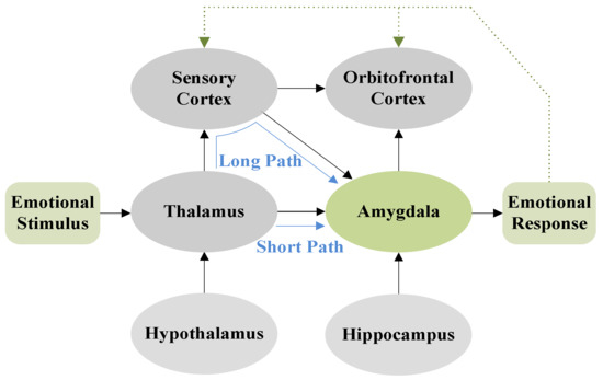
Figure 1.
Schematic diagram of the amygdala interaction with other brain systems in the limbic system.
In the LiAENN from Figure 2, the amygdala and OFC module are expanded into two layers with two hidden neurons and single output neuron by using biases bs and activation function f to introduce the anxiety-confidence emotional states into the network [30]. The emotional stimuli Pq (q = 1,...,n) as the input patterns enter into the thalamus and then go to the sensory cortex. Amygdala receives the input information from the sensory cortex. The thalamus also maps the expanded signals Pn+1 extracted from input information directly to the amygdala. The emotional output of amygdala is Ea. The OFC produces the emotional output Eo, which is to inhibit the inaccurate emotional response of the amygdala and determine the final emotional output E. The dashed line in Figure 1 and Figure 2 represent the feedback effects of resultant emotional response. In the LiAENN, the target value of input pattern T which controls the feedback effects is employed to adjust the amygdala weights vs and the OFC weights ws. Additionally, to control the effects of using targets, the network uses a decay rate to simulate the oblivious characteristic of amygdala.
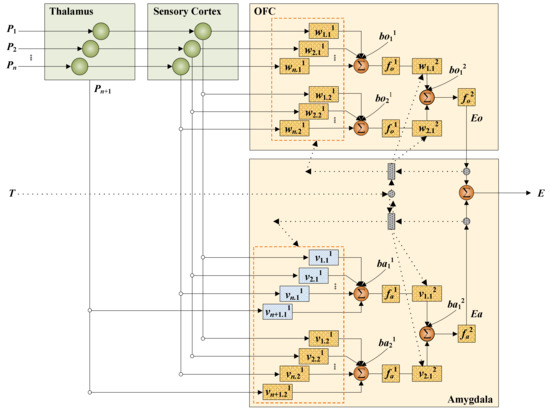
Figure 2.
Limbic-based artificial emotional neural network (LiAENN) architecture.
The LiAENN is trained with the anxious confident decayed brain emotional learning rules (ACDBEL), wherein the added anxiety-confidence emotional state and their attentional effects are used in learning in the amygdala. The emotionally derived concepts in LiAENN provide a new direction for its application in the ultra-short-term prediction of PV power.
2.2. Limitations of the Current Limbic-Based Artificial Emotion Neural Network
2.2.1. The Limitations of the Expanded Signal
The existence of the short path not only allows the model to react faster to a wide range of stimuli, but also provides another pathway for emotional learning if the long path is damaged. However, inappropriate expanded signals also bring greater challenges to the application of prediction such as interfering with other input information or leading to the redundancy of information. The two-layer architecture of LiAENN has two short paths, which increases the inaccuracy of the information transmitted through the short paths. The expanded signal, which is transmitted through the short path, is usually calculated using a nonlinear function such as a mean operator or a max operator. A mean operator represents the average value of the input signals, which is used to simulate the average trend of input signals. A max operator, which is the maximum value of input signals, is chosen to simulate the expanded signal in most ENNs. Although the applications of ENNs are becoming more and more mature, the expanded signal is still not clearly defined as to whether it is a uniform regulation or a choice based on a particular application. However, the precise definition of the extended signal is critical to the accuracy of the prediction. In this paper, the expanded signal is considered according to the chaotic characteristics of PV power time series and the prediction mechanism.
2.2.2. The Limitations of the Emotional Parameters
The LiAENN is distinctive because more emotional concepts are involved in the emotional computing. The added emotional parameters referring to the anxiety and confidence more closely mimic the attentional behavior of human learning. The confidence and anxiety variables are influenced by the perceived objects. Emotional psychology theory holds that the new learning task will bring a high initial anxiety level and low confidence level. Rather, the proficiency of practice will lead to a lower level of anxiety and a higher level of confidence. Confidence makes the previous update occupy a dominant position. Anxiety has an effect on enhancement, including latest errors, which effectively slows down the learning of new tasks. Hence, anxiety can be seen as a feature of attention focusing on learning about new and "interesting" data. The choice of these data should be considered in terms of the interaction mechanism between emotion and attention. The amygdala is responsible for attentional behavior, which can eliminate interference items from desired target objects to obtain the salience. The interaction mechanism between emotion and attention can be summarized as follows: the attention is the first step in emotion processing, and on the contrary, emotional function helps to guide attention to a great extent. The important role of the amygdala in attention and memory suggests that the quick low-level automatic emotional responses are derived from the most important stimuli associated with survival [31]. Hence, these new and "interesting" data should be determined according to the specific application. On the facial detection and emotion recognition experiments, the new and "interesting" data are resourced from the average value of the global input signals, whose goal is to mimic trends in human emotional judgments and preferences based on general impressions, rather than precise details of perceived objects.
The fluctuation of wind power is mainly reflected in the hourly fluctuation, whereas the PV power has stronger fluctuation in a few minutes. Therefore, for the ultra-short-term PV power prediction, the global average of the input signals does not provide the most direct stimulus to the emotional learning of the network. It is especially important to pick out the most important information about the prediction from the input signals. The improvement of LiAENN concentrates on tracking the detailed information of input signals, which is crucial for ultra-short-term PV power prediction. The construction of emotion parameters has a relatively certain local basis based on the chaos theory.
2.3. The Localized Emotion Reconstruction in the Limbic-based Artificial Emotional Neural Network
2.3.1. Chaotic Time Series Analysis
If the behavior of the observed time series data is chaotic, it can be assumed that the behavior follows a certain deterministic law in the high-dimensional phase space. Considering the chaotic characteristics of PV power helps to better explore the relationship between emotion and attention. The key point of this approach lies in the phase space reconstruction of the dynamics, which is aimed at mapping these historical time series into high-dimensional phase space, and then extracting and restoring the original law. The original law is a kind of trajectory in high-dimensional space, which is called chaotic attractor [32].
For a chaotic system, the phase space is defined as a vector space Rm, where each point is represented by an m-dimensional vector r(t), which is expressed as:
where t is the index of the time series and m is the dimension of the vector space.
According to Taken’s embedding theorem, the value of r(t) and its related components are unknown in the chaotic system. However, the evolution of any component of the system can be determined by other components interacting with it, so the information of these related components is implicit in the development of any components. This means that if a single quantity or variable x(t) can be observed from a chaotic system, the chaotic attractor can be recovered from the reconstructed dynamics of a system after a certain time delay , which are geometrically similar to the original attractor. Therefore, the reconstructed phase space can be used to reflect the unknown dynamics of the actual system [33]. The future value of system at time can be determined by the following equation with the nonlinear function f: , which describes the system:
where the arrows appearing in the text represent a mapping from one-dimensional space to multi-dimensional space.
Thus, although the PV power time series is random, its deterministic behavior can be described in the embedded phase space. The first step in reconstructing the PV power chaotic time series into phase space points is to determine the embedding dimension m and delay time based on the embedding theorem. Due to the small amount of calculation and strong anti-noise performance, the C-C method is used to calculate the phase space reconstruction parameters [23]. It is a kind of time delay window technique based on time series. The delay time is obtained by multiplying the delay amount and the sampling time . Taking into account the discreteness of the sampling data, we use the delay amount instead of delay time .
First, the correlation integral of PV power time series is given as follows:
where N is the length of time series; M is the number of delay vectors; is defined as the spatial distance; and H(a) is a step function, i.e., H(a)=0 if ; 1 otherwise. Xe and Xf are the random point vectors of the PV power output time series in the reconstructed phase space. Infinite norm is used to calculate the Euclidean distance between Xe and Xf. The BDS (Brock-Dechert-Scheinkman) statistic is applied to obtain the appropriate estimation of m and rd. Choose:
where and is the standard deviation of the time series.
Second, the PV power output test statistics are computed. Considering the limited sequence length and the possible relationship among the time series data points, we divide the PV power output time series into l sequences with a length . We define as an intermediate variable. The system test statistics can be found when is large enough (or approaches the infinity in theory):
The first zero crossing of is selected as the optimal delay amount of PV power output time series phase space reconstruction. Get the difference between the maximum value and the minimum value of for given the same and . is defined as the average value of the difference with different dimension , i.e.,
On account of the finite length and noise effect of the time series data, may not reach a zero-crossing point. Then, the first local minimum value of can be chosen to determine optimal delay amount in the time series phase space reconstruction. A new statistic is then defined as:
Determine the global minimum value of , which corresponds to the average trajectory cycle optimal estimate . We have the best dimension .
Then, the PV power time series can be embedded in m-dimensional space by plotting the delay vector X:
2.3.2. The Single-Step Cyclic Scrolling Localized Prediction Mechanism
The single-step cyclic scrolling localized prediction mechanism [34] is described as follows: x(t1) is assumed as the first power to be predicted and the x(t0) is the known quantity. When the power x(t1) is to be predicted at time t1, the correspondence between X(t0) and x(t1) is as follows:
where the arrow represents the corresponding relationship between input and output when the model predicts the power value x(t1) at time t1.
Then, the delay vector X(t0) is imported into the trained model, and the single-step prediction is performed. Hence, the predicted power x(t1)preat t1 time is obtained.
When the power at t2 time is to be predicted, considering that at t2 time, the actual PV power x(t1)real at the t1 time is available, the x(t1)real can be added to the last position of the phase space vector X(t1) (x(t1)=x(t1)real). Based on the phase space reconstruction, a new chaotic phase space based on x(t1) is constructed as follows:
Then, the delay vector X(t1) is imported into the trained model, and the power x(t2) at t2 time can be predicted. The effect of rolling forward one step is realized, and the cycle is used to realize the ultra-short-term prediction of every moment in the future day. The pattern-target samples extracted from PV power chaotic time series are shown in Table 1 and the whole prediction mechanism is shown in Figure 3.

Table 1.
The pattern-target samples extracted from photovoltaic (PV) power chaotic time series.
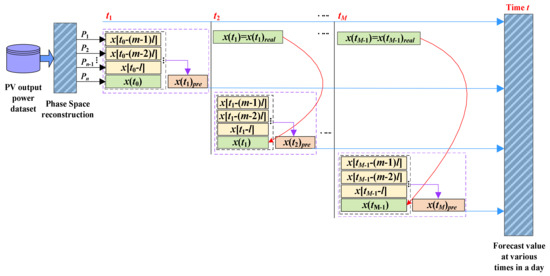
Figure 3.
The block diagram of the single-step cyclic scrolling localized prediction mechanism.
It is worth noting that each update forms a new set of chaotic phase space points, and the only unknown value in the actual prediction process refers to the last phase space point of each delay vector, which can be defined as prediction center point. The mapping relationship is more precise. This prediction mechanism ensures that the model can be adjusted by pattern-target samples and the next predicted value is not affected by the previous predicted value, which avoids the problem of error accumulation in rolling prediction.
2.3.3. The Localized Emotion Reconstruction
A. Expanded Signal
Based on aforementioned analysis, the actual prediction process can be described as a localized rolling prediction between a single delay vector with m input components and one output component. The mapping relationship shown in Table 1 indicates that the prediction center point is critical to the prediction value, which can be chosen as the expanded signal. The expanded signal is expressed as follows:
B. Emotional Parameters
The motivation for modifying these emotional parameters is our human cognitive process of new learning tasks. For the ultra-short-term prediction of PV power, the delay vector X is a time-dependent sequence transformed from the initial observation x(i) after stretching and folding. According to the prediction mechanism and the embedding theorem, the network tracks one pattern at a time. The anxiety level is affected by each pattern-target sample which is exposed to the network, and the effect of each component of single pattern on anxiety level increases with time. The predicted value is determined by x(tj) to a large extent. Based on the above analysis, the emotional parameters can be successfully modeled within the network configuration by paying attention to the details of each pattern-target sample instead of the general impression.
The anxiety coefficient and confidence coefficient can be expressed as and . The initial values of the anxiety coefficient and the confidence coefficient are set to “1” and “0”, respectively, which means that a new learning task such as first iteration needs more attention to be devoted to the learning of prediction model. With the deepening of learning or the increase of iteration steps, the decrease of anxiety level means that the derivative of the error of the training patterns is less and less valued by the network. On the contrary, increasing attention has been attached to the previous changes of network that confidence level made to weights. Therefore, the minimization of the error brings about a high level of confidence and a low level of anxiety. The anxiety and confidence maintain a balance of attention between previous iteration and subsequent iteration.
The anxiety coefficient at each time can be expressed as follows:
The err feedback of each pattern-target sample at each time is defined as:
Then the final anxiety coefficient at the -th iteration can be calculated as:
The value of confidence coefficient at the -th iteration is defined as:
where is the value of anxiety coefficient at the first iteration.
After the localized emotion reconstruction, the prediction model is trained to capture the functional relationship among given phase space points. Finally, the weights and biases of the trained model are maintained to predict the future values of the phase space points. The future values of time series are obtained when the unknown phase space points are predicted. Only the amygdala involves the emotional states, and the above process is presented in Figure 4.
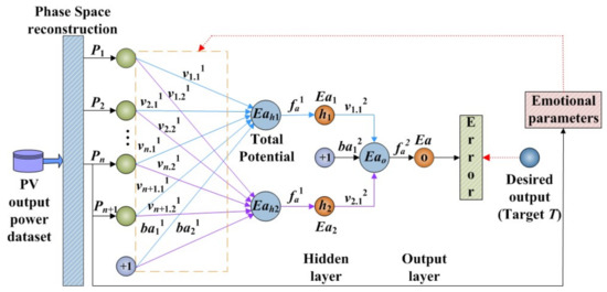
Figure 4.
The localized emotion reconstruction in the amygdala part of the localized emotion reconstruction emotional neural network (LERENN).
3. Ultra-Short-Term Photovoltaic Power Prediction Model Based on the Localized Emotion Reconstruction Emotional Neural Network
3.1. The Training Algorithm of the Localized Emotion Reconstruction Emotional Neural Network
3.1.1. Feed Forward Computations
For the amygdala, the detailed steps are as follows:
i. Input Layer to Hidden Layer
In Figure 4, the delay vector X(tj) (j = 0,1,...,M–1) as the n inputs Pq (q = 1,...,n) enter the amygdala, which come from the sensory cortex; meanwhile, the expanded signal Pn+1 as another input enters the amygdala. For the amygdala, hi is the i-th (i = 1, 2) neuron in the hidden layer. is the i-th bias neuron in the hidden layer, which is set to “+1.” Eahi is the weighted sum of the inputs to the i-th neuron in the hidden layer, which can be expressed as in Equation (17). is the activation function of the hidden layer. Eai is the activated value of the i-th neuron as the final output of hidden layer, which can be expressed as in Equation (18). is the amygdala weight associated with the connection between the q-th neuron in the input layer and the i-th neuron in the hidden layer.
ii. Hidden Layer to Output Layer
Similarly, the output value of output layer in amygdala is calculated as follows:
where (i = 1, 2) is the amygdala weight in the output layer located between the i-th neuron in the hidden layer and the output neuron; is related to the bias neuron in output layer; is the activation function of the output layer.
In the same way, the output Eo of OFC can be obtained, and the final output can be calculated by the following equation:
3.1.2. Backward Learning Computations
The backward learning computations are aimed at updating the learning weights of the amygdala and the OFC, which is similar to the error back propagation algorithm.
As can be seen from Figure 2, the output error of the amygdala is err, as shown in Equation (22):
where T is the target value, and the err actually has a result of the feed forward calculations, and the amygdala is Ea.
The aim of the training process is to minimize this error over training patterns. For the output layer neuron, a quantity called the error signal is represented by , which is expressed as:
For the first hidden neuron, an error signal definition is as follows:
Then, the learning weights of the first hidden neuron are calculated by the following equation:
Particularly, due to the expanded single from the thalamus,
where and are updated based on Equations (13)–(16) at each iteration, is the learning coefficient, and is the decay rate in amygdala learning rule. The and are adjusted as follows:
The updating between the second hidden neuron and the output neuron is similar to the backward learning computations of the OFC, and so details are no longer given here.
3.2. The Ultra-Short-Term PV Power Prediction Framework Based on the Localized Emotion Reconstruction Emotional Neural Network
After collecting the PV power time series data, the prediction can be implemented with the following steps:
(a) After data normalization, the phase space reconstruction of the obtained PV power time series is performed.
(b) Construct the localized emotion reconstruction emotional neural network (LERENN)-based model; the overall frame structure of the prediction model, especially the number of input nodes and output nodes, is determined based on the data matrix of phase space point vector. Additionally, the initial values of the emotional parameters are set.
(c) Import the phase space points to the model; the proposed model is trained with the pattern-target pairs to capture the functional relationships among the given phase space points. The total training process includes the feed forward computations, emotional parameter settings, and backward learning computations. Among them, the setting of emotional parameters is carried out in accordance with 2.3.3.
(d) The weights and biases of the trained model are maintained to predict the future values of the phase space points.
(e) Repeat the above steps to perform prediction.
The corresponding prediction process of PV power based on the proposed model is shown in Figure 5.
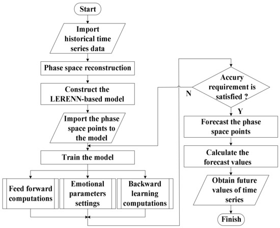
Figure 5.
The flow chart of PV power ultra-short-term prediction based on LERENN.
4. Case Study
4.1. Description of Dataset
The grid-connected PV power station built by the National Institute of Standards and Technology (NIST) in Gaithersburg, MD campus can provide the high-resolution, low uncertainty, comprehensive PV output power data for extended, continuous time periods. There is a single inverter at the station that is connected to the local grid via the NIST campus grid [35]. In this paper, the data of 70 days in the third quarter of 2015 were selected for simulation. Sampling was done daily from 6:00 am to 7:00 pm every 5 min, and 157 sampling points were included in one day set. In order to obtain an appropriate prediction accuracy with an affordable computation burden, historical data of 62 days were used as the training dataset, and 8 days of data under different weather conditions were chosen as the forecasting dataset. The training dataset includes different weather conditions, and all the dataset only includes historical PV power data. To reflect the prediction performance of the proposed model, the selected forecasting dataset include 2 sunny days, 2 cloudy days, 2 overcast days, and 2 abrupt weather days like sunny to cloudy and cloudy to sunny weather [36]. For this dataset, the ultra-short-term PV power prediction was carried out with the step length of 5 min.
To quantify errors, the mean absolute percentage error (MAPE) and the root-mean-squared error (RMSE) were used as the main two metrics. In particular, MAPE and RMSE are defined as follows:
where and are the s-th value in the predicted time series and the actual series of measured PV power, respectively, and N denotes the number of samples in test set.
However, since in some extreme weather conditions or at certain points in time, the actual PV power may fall to zero, the sum of squares due to error (SSE) defined by Equation (32) was used to represent the error in PV power prediction.
The above three evaluation metrics give the prediction information of point-wise error, however, they are not sufficient to distinguish the prediction behavior between different prediction methods. In the variability of PV power, repercussions from large ramping events are of primary concern. Hence it is useful to use ramp metric to quantify the ability of prediction methods to capture the ramp events. In this paper, we use the Ramp score proposed by Vallance et al [37] as another metric. The Ramp metric is defined as follows:
where SD(T(t)) and SD(R(t)) are the slopes of the test series and real series ramps, respectively, and the tmax and tmin are the bounds of the period to be predicted.
4.2. Benchmark Models for Numerical Comparison
For comparison, the proposed model was compared with a persistence model (PM) [38] commonly used as a benchmark model for ultra-short-term PV power prediction. In addition, the performance of the LSTM-based model, LiAENN-based model and the BPNN-based model were also compared to the proposed model.
It is noteworthy to mention that for a fair comparison, the setting of key parameters was tested in the search of optimum values. For the proposed model, the statistic curve obtained with the C-C method is shown in Figure 6.
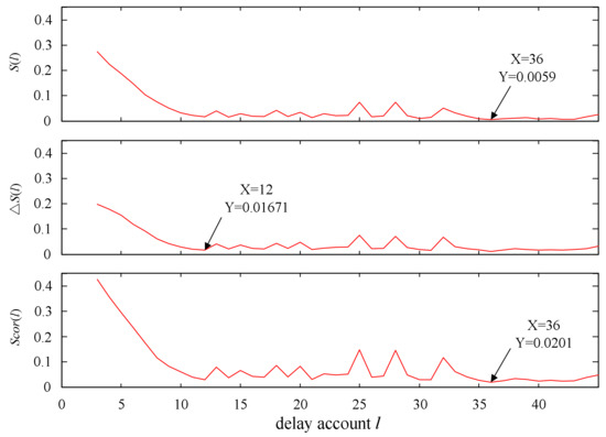
Figure 6.
Statistic curves of PV power output time series using C-C methodNote: The C-C method is a kind of time delay window technique based on time series.
As can be seen from Figure 6, since has no zero crossing, the first local minimum value of can be chosen to determine optimal delay amount in the time series phase space reconstruction. Determine the global minimum value of , which corresponds to the average trajectory cycle optimal estimate . From it, we have and . We then calculate the optimal dimension via Equation (8).
For decay rate , due to the sensitivity of the PV power chaotic system to the initial value, the should be set as a relatively small value. Take values at intervals of 0.05 within 0 to 1, and each training is repeated 10 times. = 0 is unreliable, meaning that the model barely learns new pattern-target samples during each training iteration. With the continuous increase of , the error jump range increases, and finally, the performance of the model tends to be unstable. When = 0.55, the training fails. Then, constrain the range of from 0 to 0.05 with step size 0.01. Finally, the value 0.01 is achieved as the optimum decay rate. For the BPNN-based model, we choose BPNN with three-layer network structure, the logsig function is used for the neural-transfer function of hidden layer, and the purelin function is used for the neuron transfer function of output layer. The weights and thresholds of the network are initialized by rand function. The number of neurons in the hidden layer is determined by trail according to the empirical formulas [39]. Namely, that,
where G, l, H are the number of neurons in the input layer, the hidden layer, and the output layer, respectively; and a is a constant between 0–10.
Here, eight different structures (5-9-1; 5-10-1; 5-11-1; 5-12-1; 5-13-1; 5-14-1; 5-15-1; 5-16-1) of the BPNN-based model were considered. For each structure, the experiment was repeated 20 times, and the results are presented in Table 2.
Table 2.
Comparison of the back propagation neural network (BPNN)-based model architecture.
As can be seen from Table 2, the best architecture of the BPNN-based model for PV power prediction is 5-11-1 (5 inputs, 11 hidden neurons, and 1 output). Table 3 lists the final parameters of the successfully trained models, including the BPNN-based model, the LiAENN-based model, and the proposed model.
Table 3.
The final training parameters used in the BPNN-based model, the limbic-based artificial emotional neural network (LiAENN)-based model, and the proposed model.
4.3. Numerical Results and Analysis
The simulations were carried out, aimed at testing the performance of the proposed model and comparing its performance with the benchmark models. Training and testing of the prediction models were implemented in MATLAB. For a fairer comparison, each model was run 30 times independently.
Figure 7 shows the prediction results of PV power under five typical weather conditions. It is clear that the five prediction models coincide well with the actual value in sunny weather from Figure 7b,c. It can be seen from the Figure 7b that the actual power curve is not completely smooth, so the prediction curves of each prediction model have different degrees of deviation throughout the prediction interval. Between 6:00 am to 7:00 am and 15:00 pm to 19:00 pm, the prediction results of the LiAENN-based model and the BPNN-based model both show significant deviations, and the BPNN-based model is the most significant. The prediction results of the PM and the proposed model are relatively close. Overall, the prediction curve of the proposed model is closer to the actual curve. However, the prediction error of the LSTM-based model, PM and the proposed model is mainly reflected in the stage of steep rise and fall of power. In order to further compare the prediction performance of the three prediction models, the prediction curve of the stage with large power fluctuation between 11:00 and 12:00 was selected to be enlarged. From the partial enlarged drawing, it can be seen that each prediction model has a certain lag when tracking PV output. During the power climbing phase, the predicted value is generally lower than the actual value, and during the power decline phase, the predicted value is generally higher than the actual value. The strong inertia effect of the PM model in a short period of time makes the dislocation between the predicted curve and the actual curve most obvious. Compared with the proposed model, the prediction error increases significantly. Compared with the LSTM-based model, the prediction ability of the proposed model at the power inflection point is better than that of LSTM model, which can detect ramp events better. The PV output power curve of Figure 7c is smoother than that on the first sunny day. The large prediction deviation of the benchmark models appears near the peak value. Combining two sunny test days, the proposed model outperforms all of the benchmark models in sunny weather.
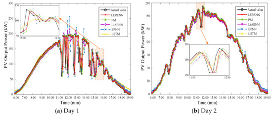
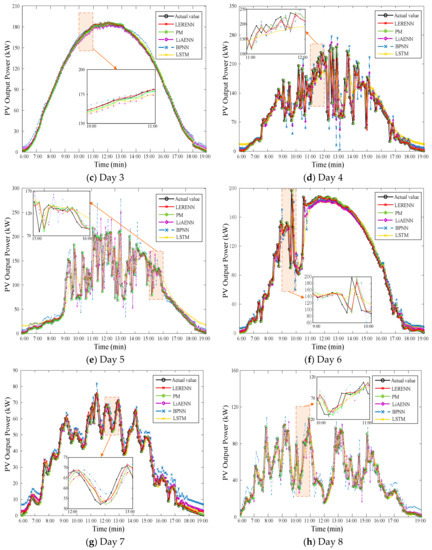
Figure 7.
The results of single-step prediction of PV power in different weather conditions.
In abrupt weather, the clouds change suddenly, and the PV power suddenly rises or falls with large fluctuation. The prediction results of each model fluctuated to a large extent. In the power smoothing phase, each model coincides well with the actual value. In the stage of large power fluctuations, as shown during 11:00 am to 16:00 am in Figure 7a and 9:00 am to 11:00 am in Figure 7f, both the LiAENN-based model and the BPNN-based model have large prediction errors. From the partial enlarged drawings, it can be seen that when the power rises and falls sharply, the prediction curve of the LSTM-based model is smoother than that of the proposed model, and the ability to detect slope events is poor. Although the prediction results based on the PM can reflect the overall trend of PV power, due to the inertia effect of the PM, when the PV power sharply rises and falls, especially at the inflection point, the tracking effect is obviously inferior to the proposed model. The proposed model can still track the original power curve well, although its prediction curve has some fluctuations. This shows that reconstructing the chaotic phase space to extract the original PV power information, and reconstructing the extended signal and emotional parameters, makes the model more sensitive to abrupt changes and fluctuations of PV power.
On cloudy days, effected by the randomness behavior of the clouds, power fluctuates greatly as the PV output is large and the prediction performance of each model is the worst in cloudy weather. From Figure 7d,e and the partial enlarged drawings, it can be seen that the proposed model still outperforms all of the benchmark models, and the BPNN-based model performs the worst. It is shown that the proposed model successfully eliminates large prediction errors, especially when the PV power fluctuates sharply.
On overcast days, the PV output is low, and the PV power fluctuation is relatively small as the cloud cover is relatively uniform. From Figure 7g,h, it can be clearly seen that the predicted values of the four models are generally smaller than the actual values in the power climbing stage. The predicted values of the four models are generally larger than the actual values in the power downhill stage. The prediction deviation is mainly reflected near the peak points and valley points; the BPNN-based model is the worst, followed by the LiAENN-based model. From the partial enlarged drawings, overall, the prediction curves of the proposed model, LSTM-based model and PM are close to each other. The prediction curve of the proposed model is closer to the actual curve means that the proposed model can improve the prediction accuracy of PV output on overcast days, but the accuracy is limited. There is still room for improvement.
To closely compare the effectiveness of the proposed model and the benchmark models, the comparison of prediction errors among different models under different weather conditions is summarized in Table 4. As can be seen from Table 4, the prediction performance of each model has the least difference in sunny weather. The proposed model outperforms all of the benchmark models under different weather conditions in general, except for individual metrics that are slightly higher than those of the LSTM-based model and PM, which are shown in bold font in the table. Focusing on the average of four metrics under various weather conditions in Table 5, the improvement in the average MAPE of the proposed model with respect to the other four models is 27.84%, 23.04%, 31.65%, and 44.90%; the improvement in the average RMSE of the proposed model with respect to the other four models is 1.82%, 7.25%, 13.77%, and 22.81%; the improvement in the average SSE of the proposed model with respect to the other four models is 2.58%, 12.71%, 23.93%, and 37.38%; the improvement in the average Ramp score of the proposed model with respect to the other four models is 30.85%, 19.55%, 31.48%, and 42.84%.
Table 4.
Comparison of single-step prediction errors among different models under different weather conditions.
Table 5.
Average value of indicators for PV power single-step prediction under different weather conditions.
As a comparison, the distributions of relative error for the proposed model and benchmark models over an 8-day period are depicted in Figure 8. The percentage of the relative error is divided into 10 bins and the reduction in prediction error is highlighted in the figure. The largest proportion of reduction in prediction errors associated with the proposed model lies in the first bin; compared with the LSTM-based model, PM, LiAENN-based model and BPNN-based model, it has 9.24%, 5.34%, 14.89% and 20.39% improvement, respectively. This result validates the effectiveness of the LERENN-based model in reducing large prediction errors.
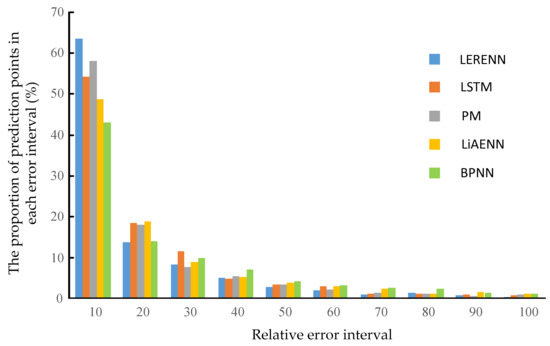
Figure 8.
The distribution of each error interval for single-step prediction.
At present, the minimum time resolution of power dispatching is 15 min. To verify prediction performance comprehensively, the three-step prediction of the first, second, fourth, sixth and seventh test days was implemented.
In order to analyze the performance of each model for the three-step prediction, the prediction errors of the four models under different typical weather conditions are given in Table 6.
Table 6.
Comparison of three-step prediction errors among different models under different weather conditions.
As can be seen from Table 6, except on overcast days, the proposed prediction model has individual metrics slightly higher than the LSTM model. Overall, the proposed prediction model has the highest prediction accuracy, and it can still detect ramp events well. Comparing Table 4 and Table 6, the prediction accuracy of all five of the models deteriorates, along with the increase of the prediction steps. The deterioration of each model is different. Compared with single-step prediction, in three-step prediction the RMSE mean value of the proposed model, the LSTM-based model, PM, the LiAENN-based model, and the BPNN-based model are increased by 17.30%, 19.67%, 21.32%, 20.29% and 23.98%, respectively. Overall, the prediction performance of the BPNN-based model is the worst. The proposed model is less affected by the increase of the prediction steps. Namely, the proposed model can improve the prediction accuracy, and it is still robust to power fluctuations and weather changes.
5. Conclusions
In this paper, a prediction model based on the localized emotion reconstruction emotional neural network for ultra-short-term prediction of PV power was proposed. Based on chaotic time series analysis, the chaotic phase space reconstruction method was used to draw the hidden characteristics of PV power time series, and the single-step cyclic rolling localized prediction mechanism was derived. The extended signal and emotional parameters were determined by the reconstructed phase space points, which have relatively sure local foundations.
Compared to the BPNN-based model, the more emotionally derived concepts in the neural network make the learning of the model more intelligent. Compared to the LiAENN-based model, the reconstructed emotional parameters and expanded signals based on the chaotic time series analysis make the model pay more attention to track each input pattern and pick out the most useful information of input pattern, with the result that the mapping relationship is more precise. Compared with LSTM-based model, the combination of chaos theory and emotion theory makes the proposed model has stronger prediction ability of ramp events. Simulation results validate that the proposed model has certain adaptability under different weather conditions.
Although in a real-world application, the utility company may argue that five minutes power prediction is less applicable since smoothing the power quality is not an easy task. In consideration of point-wise accuracy, other metrics should be considered in the next step to provide more comprehensive information in PV power prediction. In addition, meteorological factors such as solar radiation intensity and aerosol index can be used as new model inputs to further correct the prediction results. All above those are useful for the future research on the smoothing control strategy of the grid-connected PV generation system’s power output using the prediction results combined with the energy storage system.
Author Contributions
Conceptualization, Y.W. and L.Z.; methodology, Y.W. and L.Z.; software, L.Z.; validation, L.Z.; writing—original draft preparation, L.Z.; writing—review and editing, Y.W., H.X. and L.Z. All authors have read and agreed to the published version of the manuscript.
Funding
This research was funded by the Natural Science Foundation of China under Grant 61873159, the Shanghai Municipal Science and Technology Commission’s Local Capacity Construction Plan under Grant 16020500900 and the Shanghai Science and Technology Innovation Action Plan under Grant 19DZ2204700.
Conflicts of Interest
The authors declare no conflicts of interest.
References
- Engerer, N.; Mills, F. KPV: A clear-Sky index for photovoltaics. Sol. Energy 2014, 105, 679–693. [Google Scholar] [CrossRef]
- Antonanzas, J.; Osorio, N.; Escobar, R.; Urraca, R.; Martínez-De-Pisón, F.; Antonanzas-Torres, F. Review of photovoltaic power forecasting. Sol. Energy 2016, 136, 78–111. [Google Scholar] [CrossRef]
- Gigoni, L.; Betti, A.; Crisostomi, E.; Franco, A.; Tucci, M.; Bizzarri, F.; Mucci, D. Day-Ahead Hourly Forecasting of Power Generation From Photovoltaic Plants. IEEE Trans. Sustain. Energy 2017, 9, 831–842. [Google Scholar] [CrossRef]
- Agoua, X.G.; Girard, R.; Kariniotakis, G.; Kariniotakis, G. Short-Term Spatio-Temporal Forecasting of Photovoltaic Power Production. IEEE Trans. Sustain. Energy 2017, 9, 538–546. [Google Scholar] [CrossRef]
- Wang, J.; Zhong, H.; Lai, X.; Xia, Q.; Wang, Y.; Kang, C. Exploring Key Weather Factors From Analytical Modeling Toward Improved Solar Power Forecasting. IEEE Trans. Smart Grid 2019, 10, 1417–1427. [Google Scholar] [CrossRef]
- Zhen, Z.; Pang, S.; Wang, F.; Li, K.; Li, Z.; Ren, H.; Shafie-Khah, M.; Catalao, J.P.S. Pattern Classification and PSO Optimal Weights Based Sky Images Cloud Motion Speed Calculation Method for Solar PV Power Forecasting. IEEE Trans. Ind. Appl. 2019, 55, 3331–3342. [Google Scholar] [CrossRef]
- Tang, J.; Lv, Z.; Zhang, Y.; Yu, M.; Wei, W. An improved cloud recognition and classification method for photovoltaic power prediction based on total-sky-images. J. Eng. 2019, 2019, 4922–4926. [Google Scholar] [CrossRef]
- Xiang, Z.; Ji, W.; Hai, Z.; Jie, D.; Fang, C.; Xin, Z. Very short-term prediction model for photovoltaic power based on improving the total sky cloud image recognition. J. Eng. 2017, 2017, 1947–1952. [Google Scholar] [CrossRef]
- Gong, Y.; Lu, Z.; Qiao, Y.; Wang, Q. An overview of photovoltaic energy system output forecasting technology. Automat. Electron. Power Syst. 2016, 40, 140–151. [Google Scholar]
- Zhu, R.; Guo, W.; Gong, X. Short-Term Photovoltaic Power Output Prediction Based on k-Fold Cross-Validation and an Ensemble Model. Energies 2019, 12, 1220. [Google Scholar] [CrossRef]
- Cui, C.; Zou, Y.; Wei, L.; Wang, Y.; Chenggang, C.; Liaoliao, W.; Yadong, W. Evaluating combination models of solar irradiance on inclined surfaces and forecasting photovoltaic power generation. IET Smart Grid 2019, 2, 123–130. [Google Scholar] [CrossRef]
- Sheng, H.; Xiao, J.; Cheng, Y.; Ni, Q.; Wang, S. Short-Term Solar Power Forecasting Based on Weighted Gaussian Process Regression. IEEE Trans. Ind. Electron. 2017, 65, 300–308. [Google Scholar] [CrossRef]
- Utpal, K.D.; Kok, S.T.; Mehdi, S.; Saad, M.; Moh, Y.I.; Willem, V.D.; Bend, H.; Alex, S. Forecasting of photovoltaic power generation and model optimization: A review. Renew. Sustain. Energy Rev. 2018, 81, 912–928. [Google Scholar]
- Perveen, G.; Rizwan, M.; Goel, N. Comparison of intelligent modelling techniques for forecasting solar energy and its application in solar PV based energy system. IET Energy Syst. Integr. 2019, 1, 34–51. [Google Scholar] [CrossRef]
- Zhou, H.; Zhang, Y.; Yang, L.; Liu, Q.; Yan, K.; Du, Y. Short-Term Photovoltaic Power Forecasting Based on Long Short Term Memory Neural Network and Attention Mechanism. IEEE Access 2019, 7, 78063–78074. [Google Scholar] [CrossRef]
- Aprillia, H.; Yang, H.-T.; Huang, C.-M. Short-Term Photovoltaic Power Forecasting Using a Convolutional Neural Network–Salp Swarm Algorithm. Energies 2020, 13, 1879. [Google Scholar] [CrossRef]
- Safari, N.; Chung, C.Y.; Price, G.C.D. Novel Multi-Step Short-Term Wind Power Prediction Framework Based on Chaotic Time Series Analysis and Singular Spectrum Analysis. IEEE Trans. Power Syst. 2018, 33, 590–601. [Google Scholar] [CrossRef]
- Liu, L.; Ji, T.; Li, M.; Chen, Z.; Wu, Q. Short-Term local prediction of wind speed and wind power based on singular spectrum analysis and locality-sensitive hashing. J. Mod. Power Syst. Clean Energy 2018, 6, 317–329. [Google Scholar] [CrossRef]
- Liu, J.; Fang, W.; Zhang, X.; Yang, C. An Improved Photovoltaic Power Forecasting Model With the Assistance of Aerosol Index Data. IEEE Trans. Sustain. Energy 2015, 6, 434–442. [Google Scholar] [CrossRef]
- Akhter, M.N.; Mekhilef, S.; Mokhlis, H.; Shah, N.M.; Saad, M. Review on forecasting of photovoltaic power generation based on machine learning and metaheuristic techniques. IET Renew. Power Gener. 2019, 13, 1009–1023. [Google Scholar] [CrossRef]
- Zhu, H.; Li, X.; Sun, Q.; Nie, L.; Yao, J.; Zhao, G. A Power Prediction Method for Photovoltaic Power Plant Based on Wavelet Decomposition and Artificial Neural Networks. Energies 2015, 9, 11. [Google Scholar] [CrossRef]
- Al-Dahidi, S.; Ayadi, O.; Alrbai, M.; Adeeb, J. Ensemble Approach of Optimized Artificial Neural Networks for Solar Photovoltaic Power Prediction. IEEE Access 2019, 7, 81741–81758. [Google Scholar] [CrossRef]
- Wang, Y.; Fu, Y.; Sun, L.; Xue, H. Ultra-short term prediction model of photovoltaic output power based on chaos-RBF neural network. Power Syst. Technol. 2018, 42, 1110–1116. [Google Scholar]
- Shibata, K.; Takahashi, A.; Imai, J.; Funabiki, S. Short-Term prediction of power fluctuations in photovoltaic systems using chaos theory. In Proceedings of the 2013 IEEE Power & Energy Society General Meeting, Vancouver, BC, Canada, 21–25 July 2013; pp. 1–5. [Google Scholar]
- Milad, H.S.A.; Farooq, U.; El-Hawary, M.E.; Asad, U.; El-Hawary, M. Neo-Fuzzy Integrated Adaptive Decayed Brain Emotional Learning Network for Online Time Series Prediction. IEEE Access 2017, 5, 1037–1049. [Google Scholar] [CrossRef]
- Parsapoor, M.; Bilstrup, U.; Svensson, B. Forecasting Solar Activity With Computational Intelligence Models. IEEE Access 2018, 6, 70902–70909. [Google Scholar] [CrossRef]
- Mei, Y.; Tan, G.; Liu, Z.; Wu, H. Chaotic time series prediction based on brain emotion learning model and adaptive genetic algorithm. ACTA Phys. Sin. 2018, 67, 20–31. [Google Scholar]
- Zamirpour, E.; Mosleh, M. A biological brain-inspired fuzzy neural network: Fuzzy emotional neural network. Biol. Inspired Cogn. Arch. 2018, 26, 80–90. [Google Scholar] [CrossRef]
- Lotfi, E.; Akbarzadeh-T, M.-R. A winner-take-all approach to emotional neural networks with universal approximation property. Inf. Sci. 2016, 369–388. [Google Scholar] [CrossRef]
- Lotfi, E.; Akbarzadeh-T, M.-R. Practical emotional neural networks. Neural Netw. 2014, 59, 61–72. [Google Scholar] [CrossRef]
- Huang, X.; Wu, W.; Qiao, H.; Ji, Y. Brain-Inspired Motion Learning in Recurrent Neural Network With Emotion Modulation. IEEE Trans. Cogn. Dev. Syst. 2018, 10, 1153–1164. [Google Scholar] [CrossRef]
- Kim, H.; Eykholt, R.; Salas, J. Nonlinear dynamics, delay times, and embedding windows. Phys. D Nonlinear Phenom. 1999, 127, 48–60. [Google Scholar] [CrossRef]
- Ardalani-farsa, M. Chaotic Time Series Forecasting with Residual Analysis Using Synergy of Ensemble Neural Networks and Taguchi’s Design of Experiments. Ph.D. Thesis, Ryerson University, Toronto, ON, Canada, 2010. [Google Scholar]
- Wang, Y.; Fu, Y.; Xue, H. DMCS-WNN prediction method of photovoltaic power generation by considering solar radiation and chaotic feature extraction. Proc. CSEE 2019, 39, 63–71. [Google Scholar]
- Boyd, M. Performance Data from the NIST Photovoltaic Arrays and Weather Station. J. Res. Natl. Inst. Stand. Technol. 2017, 122, 40. [Google Scholar] [CrossRef]
- Li, F.; Li, C.; Y, Q. PV power ramp events probability modeling and assessment in multiple time scales. Acta Energi. Sin. 2019, 40, 3289–3298. [Google Scholar]
- Vallance, L.; Charbonnier, B.; Paul, N.; Dubost, S.; Blanc, P. Towards a standardized procedure to assess solar forecast accuracy: A new ramp and time alignment metric. Sol. Energy 2017, 150, 408–422. [Google Scholar] [CrossRef]
- Diagne, M.; David, M.; Lauret, P.; Boland, J.; Schmutz, N. Review of solar irradiance forecasting methods and a proposition for small-scale insular grids. Renew. Sustain. Energy Rev. 2013, 27, 65–76. [Google Scholar] [CrossRef]
- Kůrková, V. Komlogorov’s theorem and multi-Layer neural networks. Neural Net. 1992, 5, 501–506. [Google Scholar] [CrossRef]
© 2020 by the authors. Licensee MDPI, Basel, Switzerland. This article is an open access article distributed under the terms and conditions of the Creative Commons Attribution (CC BY) license (http://creativecommons.org/licenses/by/4.0/).