A Comparison of the Risk Quantification in Traditional and Renewable Energy Markets


Abstract
1. Introduction
2. Literature Review: Risk Quantification
3. Materials and Methods
3.1. Dynamics of VaR/ES with Mean and Variance Models
3.2. Risk Measures under Different Distributions
3.3. VaR Backtesting
3.4. ES Backtesting
3.4.1. Z1 Test
3.4.2. Z2 Test
3.4.3. ZES Test
3.4.4. Algorithm 1: Critical Values for ES Backtesting under Student’s t Distributions
| Algorithm 1 |
| 1. Simulation of under normal, skew-normal, Student’s t, skewed -t, GED and SGED distributions, and M = 10,000 times. The value indicates the test (). |
| 2. Calculation of the statistics, using the data simulated in step 1. |
| 3. Estimation of critical values (cv) at 5%, . |
| 4. Resampling the critical values for the different skewness, degrees of freedom and shape parameters. |
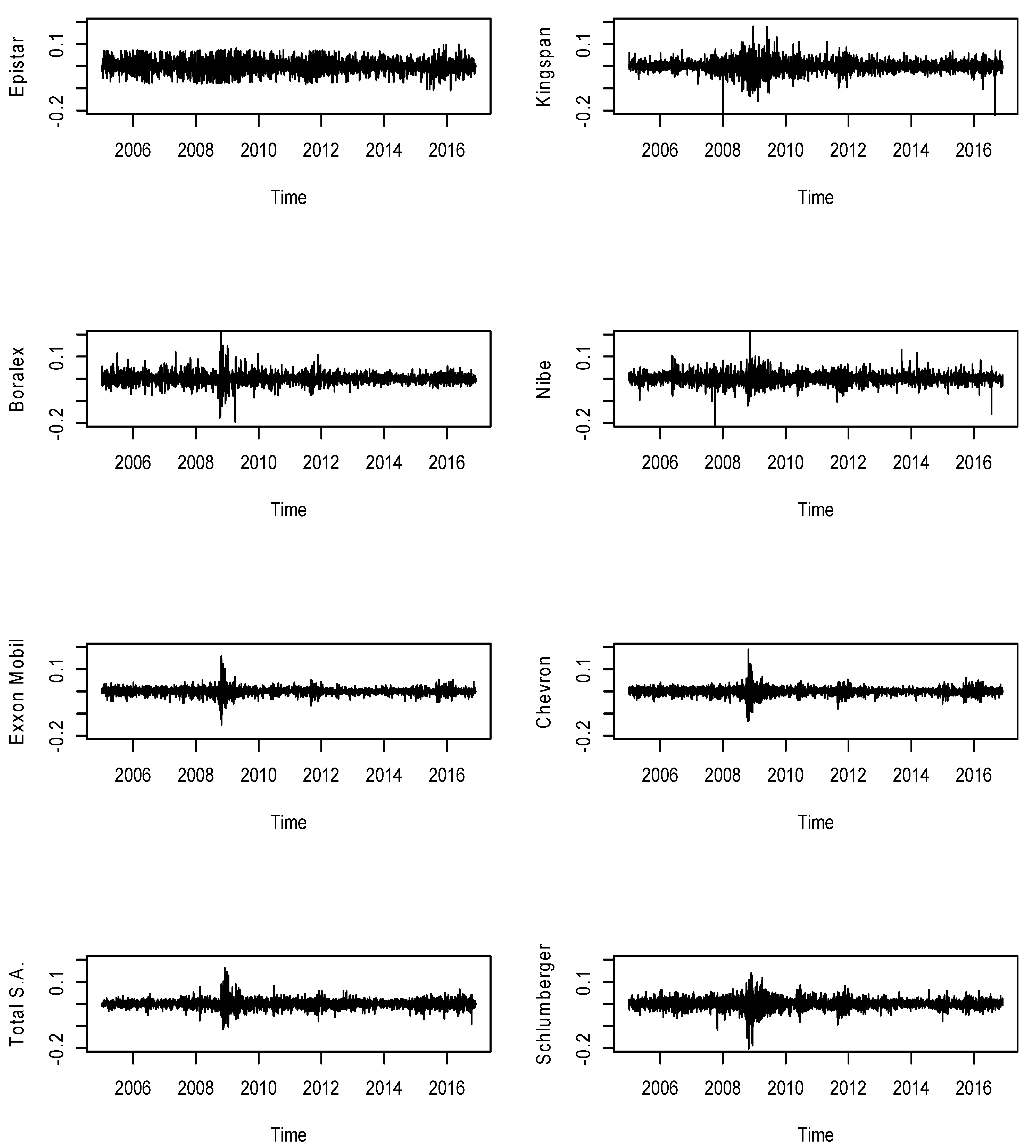
4. Data
5. Empirical Results
5.1. Conditional Mean and Variance Models in Sample Estimations
5.2. Backtesting of 99%-VaR
5.3. Backtesting of 97.5%-VaR
5.4. Backtesting of 97.5%-ES
5.4.1. Z1 Test
5.4.2. Z2 Test
5.4.3. ZES Test
6. Discussion
7. Conclusions
Author Contributions
Funding
Acknowledgments
Conflicts of Interest
Appendix A

| Stock | Index | Description |
|---|---|---|
| EPISTAR | NEX | Epistar Corporation manufactures and markets light-emitting diode (LED) chips and epitaxial wafers. The Company sells its products in Taiwan and exports worldwide. |
| Kingspan Group PLC | NEX | Kingspan Group PLC is a global market player in high-performance insulation and building envelope technologies. |
| Boralex Inc. | NEX | Boralex Inc. is an electricity producer whose core business is the development and operation of renewable energy power stations. The Corporation operates assets in the following power generation types—wind, hydroelectric, thermal and solar-based in Canada, the Northeastern United States, and France. |
| NIBE Industrier | NEX | NIBE Industrier AB is an international heating technology company. The Company is organized around three business areas, all united under a shared vision to create world-class solutions in sustainable energy. NIBE produces and sells heat pumps, boiler and water heaters, electrical heating elements as well as freestanding fireplaces. |
| Exxon Mobil Corporation | BWEI | Exxon Mobil Corporation operates petroleum and petrochemical businesses on a worldwide basis. The Company operations include exploration and production of oil and gas, electric power generation, and coal and mineral operations. Exxon Mobil also manufactures and markets fuels, lubricants and chemicals. |
| Chevron Corporation | BWEI | Chevron Corporation is an integrated energy company with operations in countries located around the world. The Company produces and transports crude oil and natural gas. Chevron also refines, markets, and distributes fuels, as well as is involved in chemical and mining operations, power generation and energy services. |
| TOTAL S.A. | BWEI | TOTAL S.A. explores for, produces, refines, transports, and markets oil and natural gas. The Company also operates a chemical division that produces polypropylene, polyethylene, polystyrene, rubber, paint, ink, adhesives, and resins. TOTAL operates gasoline filling stations in Europe, the United States and Africa. |
| Schlumberger Limited | BWEI | Schlumberger Limited is an oil services company. The Company, through its subsidiaries, provides a wide range of services, including technology, project management, and information solutions to the international petroleum industry as well as advanced acquisition and data processing surveys. |
| NEX stands for WilderHill New Energy Global Innovation index, and BWEI stands for Bloomberg World Energy index. Source: Bloomberg LP. | ||
Appendix B. Tables and Figures
| Epistar | Kingspan | Boralex | Nibe | Exxon | Chevron | Total | Schlumberger | |
|---|---|---|---|---|---|---|---|---|
| Coefficient | Normal Distribution | |||||||
| μ | 0.0000 (0.001) | 0.0000 (0.000) | 0.0000 (0.000) | 0.0000 (0.000) | 0.0000 (0.000) | 0.0000 (0.000) | 0.0000 (0.000) | 0.0000 (0.000) |
| ϕ | 0.0499 (0.019) | 0.0283 (0.020) | −0.0524 (0.019) | 0.0017 (0.020) | −0.0517 (0.019) | −0.0342 (0.019) | −0.0172 (0.019) | −0.0267 (0.019) |
| ω | 0.0000 (0.000) | 0.0000 (0.000) | 0.0000 (0.000) | 0.0000 (0.000) | 0.0000 (0.000) | 0.0000 (0.000) | 0.0000 (0.000) | 0.0000 (0.000) |
| α | 0.0414 (0.007) | 0.0952 (0.017) | 0.0319 (0.004) | 0.0931 (0.014) | 0.0812 (0.010) | 0.0837 (0.010) | 0.0758 (0.010) | 0.0496 (0.006) |
| β | 0.9433 (0.010) | 0.8894 (0.020) | 0.9659 (0.004) | 0.8652 (0.020) | 0.8989 (0.012) | 0.9012 (0.011) | 0.9074 (0.012) | 0.9428 (0.007) |
| Skew-Normal Distribution | ||||||||
| μ | 0.0001 (0.0005) | 0.0012 (0.0004) | 0.0007 (0.0003) | 0.0013 (0.0004) | 0.0004 (0.0002) | 0.0005 (0.0002) | 0.0004 (0.0003) | 0.0007 (0.0003) |
| ϕ | 0.0531 (0.0197) | 0.0298 (0.0198) | −0.0593 (0.0192) | 0.0001 (0.0207) | −0.0611 (0.0198) | −0.0409 (0.0195) | −0.0219 (0.0196) | −0.0235 (0.0198) |
| ω | 0.0000 (0.0000) | 0.0000 (0.0000) | 0.0000 (0.0000) | 0.0000 (0.0000) | 0.0000 (0.0000) | 0.0000 (0.0000) | 0.0000 (0.0000) | 0.0000 (0.0000) |
| α | 0.0405 (0.0028) | 0.0485 (0.0182) | 0.0317 (0.0022) | 0.0862 (0.0142) | 0.0857 (0.0093) | 0.0866 (0.0111) | 0.0682 (0.0095) | 0.0507 (0.0076) |
| β | 0.9435 (0.0050) | 0.9456 (0.0217) | 0.9663 (0.0020) | 0.8740 (0.0207) | 0.8945 (0.0123) | 0.8997 (0.0125) | 0.9184 (0.0119) | 0.9412 0.0089 |
| ξ | 1.0119 (0.0235) | 1.0162 (0.0221) | 1.0032 (0.0194) | 1.0340 (0.0212) | 0.9062 (0.0211) | 0.8597 (0.0225) | 0.9295 (0.0216) | 0.9729 (0.0226) |
| Student’s t Distribution | ||||||||
| μ | 0.0000 (0.000) | 0.0000 (0.000) | 0.0000 (0.000) | 0.0000 (0.000) | 0.0000 (0.000) | 0.0000 (0.000) | 0.0000 (0.000) | 0.0000 (0.000) |
| ϕ | 0.0274 (0.019) | 0.0216 (0.018) | −0.0653 (0.018) | −0.0065 (0.0019) | −0.0524 (0.018) | −0.0352 (0.019) | −0.0196 (0.018) | −0.0285 (0.018) |
| ω | 0.0000 (0.000) | 0.0000 (0.000) | 0.0000 (0.000) | 0.0000 (0.000) | 0.0000 (0.000) | 0.0000 (0.000) | 0.0000 (0.000) | 0.0000 (0.000) |
| α | 0.0500 (0.008) | 0.0446 (0.009) | 0.1131 (0.028) | 0.0883 (0.019) | 0.0831 (0.013) | 0.0805 (0.011) | 0.0689 (0.011) | 0.0478 (0.007) |
| β | 0.9421 (0.010) | 0.9497 (0.010) | 0.8494 (0.039) | 0.8762 (0.026) | 0.9026 (0.014) | 0.9089 (0.011) | 0.9151 (0.014) | 0.9484 (0.007) |
| 8.7578 (1.529) | 5.2540 (0.498) | 5.8807 (0.298) | 5.2573 (0.488) | 6.6061 (0.766) | 10.000 (1.452) | 7.6678 (1.035) | 7.8742 (1.028) | |
| Skewed-t Distribution | ||||||||
| μ | 0.0000 (0.000) | 0.0000 (0.000) | 0.0000 (0.000) | 0.0000 (0.000) | 0.0000 (0.000) | 0.0000 (0.000) | 0.0000 (0.000) | 0.0000 (0.000) |
| ϕ | 0.0286 (0.019) | 0.0216 (0.018) | −0.0653 (0.018) | −0.0030 (0.019) | −0.0572 (0.019) | −0.0427 (0.019) | −0.0268 (0.018) | −0.0285 (0.018) |
| ω | 0.0000 (0.000) | 0.0000 (0.000) | 0.0000 (0.000) | 0.0000 (0.000) | 0.0000 (0.000) | 0.0000 (0.000) | 0.0000 (0.000) | 0.0000 (0.000) |
| α | 0.0501 (0.008) | 0.0445 (0.009) | 0.1132 (0.027) | 0.0887 (0.018) | 0.0833 (0.012) | 0.0809 (0.011) | 0.0670 (0.011) | 0.0478 (0.007) |
| β | 0.9421 (0.010) | 0.9497 (0.010) | 0.8491 (0.038) | 0.8762 (0.025) | 0.9018 (0.014) | 0.9093 (0.011) | 0.9172 (0.014) | 0.9484 (0.007) |
| ν | 8.6184 (1.478) | 5.2529 (0.498) | 5.8799 (0.298) | 5.2686 (0.489) | 6.7975 (0.812) | 10.000 (1.422) | 7.6179 (1.031) | 7.8740 (1.028) |
| λ | 1.0288 (0.025) | 0.9987 (0.025) | 1.0167 (0.024) | 1.0483 (0.027) | 0.9385 (0.024) | 0.882 (0.024) | 0.9253 (0.023) | 1.0003 (0.026) |
| GED | ||||||||
| μ | −0.0003 (0.000) | 0.0009 (0.000) | 0.0003 (0.000) | 0.0007 (0.000) | 0.0005 (0.000) | 0.0007 (0.000) | 0.0006 (0.000) | 0.0007 (0.000) |
| ϕ | 0.0220 (0.019) | 0.0103 (0.019) | −0.0676 (0.015) | −0.0165 (0.019) | −0.0490 (0.019) | −0.0356 (0.019) | −0.023 (0.020) | −0.0283 (0.019) |
| ω | 0.0000 (0.000) | 0.0000 (0.000) | 0.0000 (0.000) | 0.0000 (0.000) | 0.0000 (0.000) | 0.0000 (0.000) | 0.0000 (0.000) | 0.0000 (0.000) |
| α | 0.0444 (0.004) | 0.0431 (0.008) | 0.0394 (0.006) | 0.0760 (0.017) | 0.0851 (0.013) | 0.0852 (0.012) | 0.0676 (0.012) | 0.0501 (0.018) |
| β | 0.9443 (0.006) | 0.9516 (0.009) | 0.9521 (0.007) | 0.8873 (0.027) | 0.8977 (0.015) | 0.9014 (0.014) | 0.9188 (0.015) | 0.9439 (0.021) |
| η | 1.4626 (0.053) | 1.2959 (0.046) | 1.1214 (0.038) | 1.2557 (0.041) | 1.4437 (0.051) | 1.6629 (0.061) | 1.4599 (0.054) | 1.4819 (0.056) |
| SGED | ||||||||
| μ | −0.0001 (0.001) | 0.0010 (0.000) | 0.0005 (0.000) | 0.0010 (0.000) | 0.0003 (0.000) | 0.0005 (0.000) | 0.0004 (0.000) | 0.0006 (0.000) |
| ϕ | 0.0224 (0.019) | 0.0111 (0.016) | −0.0695 (0.013) | −0.0124 (0.022) | −0.0601 (0.020) | −0.0429 (0.019) | −0.0287 (0.019) | −0.0290 (0.019) |
| ω | 0.0000 (0.000) | 0.0000 (0.000) | 0.0000 (0.000) | 0.0000 (0.000) | 0.0000 (0.000) | 0.0000 (0.000) | 0.0000 (0.000) | 0.0000 (0.000) |
| α | 0.0446 (0.004) | 0.0436 (0.009) | 0.0394 (0.006) | 0.0777 (0.017) | 0.0850 (0.013) | 0.0846 (0.013) | 0.0649 (0.012) | 0.0500 (0.018) |
| β | 0.9439 (0.006) | 0.9511 (0.010) | 0.9520 (0.007) | 0.8865 (0.026) | 0.8972 (0.015) | 0.9025 (0.015) | 0.9217 (0.016) | 0.9440 (0.021) |
| η | 1.4597 (0.023) | 1.2970 (0.020) | 1.1220 (0.019) | 1.2533 (0.028) | 1.4618 (0.023) | 1.7051 (0.023) | 1.4639 (0.023) | 1.4834 (0.025) |
| ζ | 1.0266 (0.053) | 1.0128 (0.046) | 1.019 (0.038)0 | 1.0576 (0.040) | 0.9339 (0.052) | 0.8713 (0.064) | 0.9331 (0.054) | 0.9920 (0.057) |
| Epistar | Kingspan | Boralex | Nibe | Exxon | Chevron | Total | Schlumberger | |
|---|---|---|---|---|---|---|---|---|
| Coefficient | Normal Distribution | |||||||
| μ | 0.0000 (0.0009) | 0.0000 (0.0004) | 0.0000 (0.0004) | 0.0000 (0.0003) | 0.0000 (0.0002) | 0.0000 (0.0002) | 0.0000 (0.0002) | 0.0000 (0.0003) |
| ϕ | 0.055 (0.077) | 0.019 (0.020) | −0.052 (0.020) | −0.002 (0.003) | −0.051 (0.020) | −0.022 (0.011) | −0.007 (0.019) | −0.027 (0.019) |
| ω | −2.025 (0.491) | −0.307 (0.061) | −0.390 (0.075) | −0.258 (0.027) | −0.213 (0.021) | −0.157 (0.035) | −0.335 (0.043) | −0.329 (0.045) |
| α | −0.095 (0.022) | −0.042 (0.013) | −0.069 (0.011) | −0.060 (0.011) | −0.069 (0.011) | −0.078 (0.012) | −0.104 (0.005) | −0.060 (0.012) |
| β | 0.712 (0.070) | 0.957 (0.008) | 0.948 (0.010) | 0.965 (0.004) | 0.975 (0.002) | 0.981 (0.004) | 0.959 (0.005) | 0.957 (0.006) |
| γ | 0.278 (0.019) | 0.232 (0.026) | 0.188 (0.005) | 0.154 (0.038) | 0.177 (0.016) | 0.158 (0.041) | 0.160 (0.005) | 0.178 (0.020) |
| Skew-Normal Distribution | ||||||||
| μ | −0.0001 (0.0006) | 0.0007 (0.0003) | 0.0002 (0.0002) | 0.0011 (0.0004) | 0.0001 (0.0002) | 0.0002 (0.0003) | 0.0001 (0.0003) | 0.0003 (0.0003) |
| ϕ | 0.0488 (0.0192) | 0.0219 (0.0172) | −0.0591 (0.0152) | −0.0085 (0.0196) | −0.0570 (0.0188) | −0.0232 (0.0189) | −0.0155 (0.0188) | −0.0225 (0.0191) |
| ω | −0.1515 (0.0086) | −0.0308 (0.0005) | −0.0195 (0.0004) | −0.2447 (0.0089) | −0.2277 (0.0235) | −0.1516 (0.0328) | −0.1556 (0.0089) | −0.0828 (0.0011) |
| α | −0.0324 (0.0079) | −0.0327 (0.0065) | −0.0456 (0.0047) | −0.0585 (0.0060) | −0.0700 (0.0111) | −0.0784 (0.0112) | −0.0803 (0.0107) | −0.0413 (0.0078) |
| β | 0.9782 (0.0012) | 0.9955 (0.0001) | 0.9968 (0.0001) | 0.9667 (0.0013) | 0.9731 (0.0027) | 0.9820 (0.0039) | 0.9808 (0.0011) | 0.9890 (0.0002) |
| γ | 0.0935 (0.0118) | 0.0770 (0.00275 | 0.0690 (0.0027) | 0.1481 (0.0156) | 0.1822 (0.0165) | 0.1561 (0.0423) | 0.1107 (0.0202) | 0.1008 (0.0036) |
| ξ | 1.0226 (0.0240) | 1.0219 (0.0219) | 1.0123 (0.0193) | 1.0390 (0.0211) | 0.9006 (0.0212) | 0.8569 (0.0230) | 0.9351 (0.0219) | 0.9757 (0.0226) |
| Student’s t Distribution | ||||||||
| μ | 0.000 (0.001) | 0.000 (0.000) | 0.000 (0.000) | 0.000 (0.000) | 0.000 (0.000) | 0.000 (0.000) | 0.000 (0.000) | 0.000 (0.000) |
| ϕ | 0.036 (0.020) | 0.023 (0.020) | −0.069 (0.019) | −0.007 (0.018) | −0.052 (0.018) | −0.027 (0.019) | −0.014 (0.020) | −0.025 (0.019) |
| ω | −1.491 (0.341) | −0.562 (0.605) | −1.550 (0.534) | −0.311 (0.026) | −0.150 (0.013) | −0.138 (0.029) | −0.176 (0.002) | −0.068 (0.003) |
| α | −0.095 (0.021) | −0.069 (0.029) | −0.038 (0.027) | −0.066 (0.015) | −0.063 (0.012) | −0.072 (0.013) | −0.083 (0.011) | −0.051 (0.009) |
| β | 0.788 (0.049) | 0.925 (0.081) | 0.798 (0.070) | 0.959 (0.003) | 0.983 (0.002) | 0.984 (0.004) | 0.979 (0.000) | 0.991 (0.000) |
| γ | 0.289 (0.019) | 0.290 (0.148) | 0.414 (0.035) | 0.174 (0.024) | 0.172 (0.020) | 0.150 (0.055) | 0.118 (0.009) | 0.104 (0.011) |
| ν | 9.972 (2.372) | 5.947 (0.574) | 5.621 (0.242) | 5.344 (0.505) | 7.021 (0.898) | 13.361 (5.56) | 8.410 (1.176) | 8.356 (0.801) |
| Skewed-t Distribution | ||||||||
| μ | 0.000 (0.001) | 0.000 (0.000) | 0.000 (0.000) | 0.000 (0.000) | 0.000 (0.000) | 0.000 (0.000) | 0.000 (0.000) | 0.000 (0.000) |
| ϕ | −0.008 (0.018) | 0.011 (0.018) | −0.070 (0.019) | −0.005 (0.023) | −0.057 (0.018) | −0.041 (0.019) | −0.027 (0.018) | −0.025 (0.015) |
| ω | −0.117 (0.072) | −0.132 (0.075) | −1.574 (0.530) | −0.313 (0.026) | −0.150 (0.013) | −0.350 (0.093) | −0.365 (0.110) | −0.068 (0.002) |
| α | −0.698 (0.116) | −0.558 (0.175) | −0.038 (0.027) | −0.066 (0.015) | −0.063 (0.012) | −1.083 (0.278) | −1.417 (0.200) | −0.051 (0.009) |
| β | 0.935 (0.032) | 0.942 (0.028) | 0.795 (0.070) | 0.959 (0.003) | 0.983 (0.001) | 0.889 (0.027) | 0.888 (0.032) | 0.991 (0.000) |
| γ | 2.410 (0.330) | 2.553 (0.517) | 0.416 (0.034) | 0.176 (0.024) | 0.171 (0.020) | 3.587 (0.145) | 2.464 (0.155) | 0.104 (0.011) |
| ν | 4.010 (0.001) | 5.456 (0.000) | 5.613 (0.242) | 5.354 (0.506 | 7.229 (0.957) | 5.812 (0.001) | 4.513 (0.000) | 8.357 (0.808) |
| λ | 1.034 (0.029) | 0.988 (0.023) | 1.011 (0.025) | 1.045 (0.027) | 0.935 (0.024) | 0.926 (0.028) | 0.945 (0.025) | 0.995 (0.026) |
| GED | ||||||||
| μ | −0.0005 (0.001) | 0.0007 (0.000) | 0.0002 (0.000) | 0.0004 (0.000) | 0.0003 (0.000) | 0.0003 (0.000) | 0.0003 (0.000) | 0.0004 (0.000) |
| ϕ | 0.0191 (0.014) | 0.0073 (0.015) | −0.0685 (0.021) | −0.0180 (0.020) | −0.0477 (0.021) | −0.0232 (0.019) | −0.0215 (0.019) | −0.0245 (0.019) |
| ω | −0.1301 (0.004) | −0.0371 (0.001) | −0.0612 (0.001) | −0.2399 (0.037) | −0.2105 (0.024) | −0.1526 (0.019) | −0.1609 (0.003) | −0.0761 (0.002) |
| α | −0.0328 (0.009) | −0.0337 (0.008) | −0.0395 (0.009) | −0.0613 (0.014) | −0.0688 (0.014) | −0.0772 (0.012) | −0.0800 (0.010) | −0.0471 (0.009) |
| β | 0.9816 (0.001) | 0.9952 (0.000) | 0.9922 (0.000) | 0.9684 (0.005) | 0.9759 (0.003) | 0.9823 (0.002) | 0.9807 (0.001) | 0.9903 (0.000) |
| γ | 0.1035 (0.008) | 0.0796 (0.007) | 0.0924 (0.009) | 0.1409 (0.040) | 0.1804 (0.019) | 0.1570 (0.023) | 0.1144 (0.009) | 0.1016 (0.001) |
| η | 1.4724 (0.057) | 1.3183 (0.046) | 1.1360 (0.037) | 1.2649 (0.041) | 1.4612 (0.054) | 1.7093 (0.068) | 1.5078 (0.055) | 1.4797 (0.051) |
| SGED | ||||||||
| μ | −0.0003 (0.001) | 0.0008 (0.000) | 0.0003 (0.000) | 0.0007 (0.000) | 0.0001 (0.000) | 0.0002 (0.000) | 0.0001 (0.000) | 0.0003 (0.000) |
| ϕ | 0.0181 (0.020) | 0.0075 (0.016) | −0.0698 (0.013) | −0.0159 (0.019) | −0.0579 (0.019) | −0.0275 (0.019) | −0.0239 (0.019) | −0.0254 (0.019) |
| ω | −0.1310 (0.004) | −0.0369 (0.001) | −0.0608 (0.001) | −0.2357 (0.030) | −0.2234 (0.042) | −0.1475 (0.028) | −0.1566 (0.001) | −0.0766 (0.002) |
| α | −0.0332 (0.009) | −0.0335 (0.008) | −0.0390 (0.009) | −0.0593 (0.014) | −0.0712 (0.014) | −0.0764 (0.012) | −0.0794 (0.010) | −0.0470 (0.009) |
| β | 0.9815 (0.001) | 0.9952 (0.000) | 0.9923 (0.000) | 0.9690 (0.004) | 0.9743 (0.005) | 0.9827 (0.003) | 0.9811 (0.000) | 0.9902 (0.000) |
| γ | 0.1039 (0.008) | 0.0800 (0.007) | 0.0923 (0.009) | 0.1446 (0.033) | 0.1815 (0.021) | 0.1534 (0.038) | 0.1092 (0.007) | 0.1014 (0.001) |
| η | 1.4707 (0.057) | 1.3192 (0.046) | 1.1362 (0.037) | 1.2652 (0.041) | 1.4805 (0.055) | 1.7464 (0.082) | 1.5056 (0.055) | 1.4806 (0.051) |
| ζ | 1.0310 (0.024) | 1.0063 (0.020) | 1.0131 (0.019) | 1.0514 (0.026) | 0.9247 (0.022) | 0.8641 (0.024) | 0.9294 (0.022) | 0.9879 (0.025) |
| Epistar | Kingspan | Boralex | Nibe | Exxon | Chevron | Total | Schlumberger | |
|---|---|---|---|---|---|---|---|---|
| Coefficient | Normal Distribution | |||||||
| μ | 0.0000 (0.000) | 0.0000 (0.000) | 0.0000 (0.000) | 0.0000 (0.000) | 0.0000 (0.000) | 0.0000 (0.000) | 0.0000 (0.000) | 0.0000 (0.000) |
| ϕ | 0.0463 (0.018) | 0.0145 (0.014) | −0.0511 (0.019) | 0.0019 (0.019) | −0.0529 (0.020) | −0.0246 (0.020) | −0.0151 (0.016) | −0.0218 (0.19) |
| ω | 0.0005 (0.000) | 0.0003 (0.000) | 0.0000 (0.000) | 0.0018 (0.000) | 0.0001 (0.000) | 0.0001 (0.000) | 0.0009 (0.000) | 0.0000 (0.000) |
| α | 0.0498 (0.007) | 0.0361 (0.05) | 0.0307 (0.005) | 0.0844 (0.010) | 0.0881 (0.011) | 0.0802 (0.010) | 0.0653 (0.009) | 0.0500 (0.007) |
| β | 0.9396 (0.010) | 0.9690 (0.003) | 0.9697 (0.003) | 0.9020 (0.013) | 0.8988 (0.011) | 0.9124 (0.009) | 0.9279 (0.011) | 0.9471 (0.006) |
| γ | 0.3283 (0.094) | 0.4062 (0.150) | 0.4534 (0.108) | 0.4670 (0.106) | 0.3935 (0.076) | 0.5248 (0.097) | 0.8203 (0.112) | 0.3714 (0.098) |
| δ | 1.0739 (0.263) | 0.7834 (0.253) | 1.6283 (0.232) | 0.7959 (0.159) | 1.3440 (0.214) | 1.2293 (0.202) | 0.8168 (0.167) | 1.4029 (0.226) |
| Skew-Normal Distribution | ||||||||
| μ | −0.0001 (0.0005) | 0.0007 (0.0003) | 0.0004 (0.0003) | 0.0011 (0.0002) | 0.0001 (0.0002) | 0.0002 (0.0002) | 0.0000 (0.0001) | 0.0004 (0.0003) |
| ϕ | 0.0498 (0.0215) | 0.0206 (0.0130) | −0.0590 (0.0190) | −0.0029 (0.0038) | −0.0553 (0.0196) | −0.0262 (0.0195) | −0.0167 (0.0042) | −0.0188 (0.0194) |
| ω | 0.0005 (0.0005) | 0.0002 (0.0000) | 0.0000 (0.0000) | 0.0018 (0.0012) | 0.0001 (0.0001) | 0.0001 (0.0001) | 0.0010 (0.0007) | 0.0001 (0.0001) |
| α | 0.0495 (0.0103) | 0.0373 (0.0013) | 0.0305 (0.0020) | 0.0795 (0.0108) | 0.0947 (0.0114) | 0.0807 (0.0103) | 0.0544 (0.0155) | 0.0499 (0.0066) |
| β | 0.9378 (0.0156) | 0.9675 (0.0003) | 0.9682 (0.0015) | 0.9062 (0.0132) | 0.8916 (0.0117) | 0.9118 (0.0100) | 0.9422 (0.0216) | 0.9474 (0.0061) |
| γ | 0.3413 (0.1006) | 0.4763 (0.0991) | 0.4041 (0.0759) | 0.4901 (0.1130) | 0.3914 (0.0754) | 0.4775 (0.0945) | 0.9037 (0.1513) | 0.3765 (0.1012) |
| δ | 1.0937 (0.2763) | 0.8959 (0.0482) | 1.7392 (0.0380) | 0.7835 (0.1661) | 1.3313 (0.2018) | 1.2970 (0.1934) | 0.7297 (0.2298) | 1.3378 (0.2035) |
| ξ | 1.0235 (0.0239) | 1.0258 (0.0220) | 1.0135 (0.0198) | 1.0402 (0.0215) | 0.8990 (0.0212) | 0.8575 (0.0225) | 0.9351 (0.0219) | 0.9732 (0.0226) |
| Student’s t Distribution | ||||||||
| μ | 0.0000 (0.000) | 0.0000 (0.000) | 0.0000 (0.000) | 0.0000 (0.000) | 0.0000 (0.000) | 0.0000 (0.000) | 0.0000 (0.000) | 0.0000 (0.000) |
| ϕ | 0.0240 (0.019) | 0.0169 (0.019) | −0.0660 (0.018) | −0.0056 (0.017) | −0.0516 (0.018) | −0.0295 (0.019) | −0.0196 (0.020) | −0.0228 (0.018) |
| ω | 0.0003 (0.000) | 0.0002 (0.000) | 0.0001 (0.000) | 0.0011 (0.000) | 0.0001 (0.000) | 0.0001 (0.000) | 0.0010 (0.000) | 0.0001 (0.000) |
| α | 0.0599 (0.009) | 0.0440 (0.008) | 0.1036 (0.029) | 0.0842 (0.014) | 0.0940 (0.014) | 0.0764 (0.011) | 0.0629 (0.009) | 0.0514 (0.008) |
| β | 0.9374 (0.010) | 0.9611 (0.006) | 0.8826 (0.037) | 0.9087 (0.016) | 0.8995 (0.013) | 0.9190 (0.010) | 0.9309 (0.012) | 0.9494 (0.007) |
| γ | 0.2804 (0.090) | 0.4878 (0.140) | 0.1524 (0.073) | 0.4344 (0.112) | 0.3965 (0.089) | 0.4985 (0.108) | 0.8705 (0.115) | 0.4807 (0.115) |
| δ | 1.1112 (0.253) | 0.9558 (0.173) | 1.6047 (0.266) | 0.8777 (0.182) | 1.2454 (0.235) | 1.2586 (0.227) | 0.7786 (0.180) | 1.2967 (0.230) |
| ν | 8.9644 (0.1609) | 5.4858 (0.534) | 5.9731 (0.315) | 5.3611 (0.500) | 7.0192 (0.854) | 10.000 1.381 | 8.5843 (1.272) | 8.1418 (1.068) |
| Skewed-t Distribution | ||||||||
| μ | 0.0000 (0.001) | 0.0000 (0.000) | 0.0000 (0.000) | 0.0000 (0.000) | 0.0000 (0.000) | 0.0000 (0.000) | 0.0000 (0.000) | 0.0000 (0.000) |
| ϕ | 0.0247 (0.020) | 0.0170 (0.019) | −0.0663 (0.018) | −0.0042 (0.018) | −0.0547 (0.020) | −0.0335 (0.019) | −0.0226 (0.014) | −0.0227 (0.018) |
| ω | 0.0003 (0.000) | 0.0002 (0.000) | 0.0001 (0.000) | 0.0010 (0.000) | 0.0001 (0.000) | 0.0001 (0.000) | 0.0010 (0.000) | 0.0001 (0.000) |
| α | 0.0604 (0.009) | 0.0440 (0.008) | 0.1040 (0.029) | 0.0850 (0.014) | 0.0939 (0.014) | 0.0759 (0.011) | 0.0613 (0.009) | 0.0514 (0.008) |
| β | 0.9369 (0.011) | 0.9611 (0.006) | 0.8819 (0.037) | 0.9084 (0.016) | 0.8985 (0.013) | 0.9200 (0.010) | 0.9324 (0.012) | 0.9494 (0.007) |
| γ | 0.2915 (0.091) | 0.4885 (0.141) | 0.1508 (0.074) | 0.4317 (0.112) | 0.3997 (0.089) | 0.4903 (0.108) | 0.8812 (0.116) | 0.4808 (0.116) |
| δ | 1.0959 (0.251) | 0.9560 (0.173) | 1.6053 (0.266) | 0.8782 (0.183) | 1.2520 (0.233) | 1.2570 (0.219) | 0.7915 (0.183) | 1.2972 (0.231) |
| ν | 8.8193 (1.553) | 5.4835 (0.534) | 5.9717 (0.315) | 5.3631 (0.500) | 7.2550 (0.914) | 10.0000 (1.352) | 8.4353 (1.239) | 8.1419 (1.068) |
| λ | 1.0373 (0.026) | 0.9979 (0.025) | 1.0150 (0.024) | 1.0496 (0.028) | 0.9347 (0.024) | 0.8833 (0.025) | 0.9256 (0.023) | 1.0023 (0.026) |
| GED | ||||||||
| μ | −0.0005 (0.000) | 0.0007 (0.000) | 0.0002 (0.000) | 0.0004 (0.000) | 0.0003 (0.000) | 0.0004 (0.000) | 0.0002 (0.000) | 0.0004 (0.000) |
| ϕ | 0.0192 (0.015) | 0.0069 (0.018) | −0.0684 (0.017) | −0.0151 (0.020) | −0.0483 (0.019) | −0.0270 (0.020) | −0.0245 (0.005) | −0.0232 (0.019) |
| ω | 0.0005 (0.000) | 0.0001 (0.000) | 0.0000 (0.000) | 0.0010 (0.001) | 0.0001 (0.000) | 0.0001 (0.000) | 0.0011 (0.002) | 0.0001 (0.000) |
| α | 0.0550 (0.013) | 0.0386 (0.002) | 0.0412 (0.010) | 0.0770 (0.014) | 0.0933 (0.013) | 0.0807 (0.011) | 0.0551 (0.043) | 0.0505 (0.007) |
| β | 0.9378 (0.018) | 0.9657 (0.000) | 0.9536 (0.003) | 0.9094 (0.018) | 0.8958 (0.013) | 0.9116 (0.011) | 0.9416 (0.060) | 0.9488 (0.006) |
| γ | 0.3166 (0.104) | 0.4740 (0.124) | 0.2562 (0.067) | 0.4785 (0.132) | 0.3864 (0.088) | 0.4722 (0.102) | 0.8899 (0.355) | 0.4355 (0.116) |
| δ | 1.0750 (0.289) | 0.9619 (0.060) | 1.7863 (0.045) | 0.9253 (0.210) | 1.3296 (0.232) | 1.2952 (0.218) | 0.7131 (0.607) | 1.2793 (0.223) |
| η | 1.4721 (0.059) | 1.3237 (0.046) | 1.1369 (0.038) | 1.2715 (0.041) | 1.4668 (0.052) | 1.7166 (0.064) | 1.5221 (0.056) | 1.4899 (0.052) |
| SGED | ||||||||
| μ | −0.0003 (0.001) | 0.0008 (0.000) | 0.0003 (0.000) | 0.0007 (0.000) | 0.0001 (0.000) | 0.0002 (0.000) | 0.0001 (0.000) | 0.0004 (0.000) |
| ϕ | 0.0184 (0.020) | 0.0075 (0.018) | −0.0704 (0.017) | −0.0130 (0.010) | −0.0565 (0.020) | −0.0303 (0.020) | −0.0258(0.006) | −0.0241 (0.019) |
| ω | 0.0005 (0.000) | 0.0001 (0.000) | 0.0000 (0.000) | 0.0010 (0.001) | 0.0001 (0.000) | 0.0001 (0.000) | 0.0011 (0.001) | 0.0001 (0.000) |
| α | 0.0552 (0.014) | 0.0388 (0.002) | 0.0409 (0.018) | 0.0785 (0.014) | 0.0946 (0.014) | 0.0794 (0.011) | 0.0532 (0.003) | 0.0504 (0.007) |
| β | 0.9373 (0.019) | 0.9656 (0.000) | 0.9537 (0.002) | 0.9088 (0.017) | 0.8936 (0.013) | 0.9133 (0.011) | 0.9438 (0.003) | 0.9488 (0.006) |
| γ | 0.3225 (0.105) | 0.4689 (0.124) | 0.2533 (0.011) | 0.4546 (0.124) | 0.3995 (0.088) | 0.4713 (0.101) | 0.9123 (0.024) | 0.4366 (0.116) |
| δ | 1.0626 (0.289) | 0.9603 (0.060) | 1.7912 (0.109) | 0.9259 (0.178) | 1.3185 (0.234) | 1.3070 (0.209) | 0.7026 (0.129) | 1.2759 (0.223) |
| η | 1.4705 (0.059) | 1.3252 (0.046) | 1.1374 (0.038) | 1.2718 (0.041) | 1.4876 (0.053) | 1.7570 (0.067) | 1.5176 (0.056) | 1.4911 (0.052) |
| ζ | 1.0316 (0.024) | 1.0082 (0.021) | 1.0160 (0.023) | 1.0526 (0.024) | 0.9239 (0.023) | 0.8652 (0.023) | 0.9278 (0.022) | 0.9878 (0.024) |
| Normal Distribution | |||||||||
|---|---|---|---|---|---|---|---|---|---|
| AR(1)-GARCH(1,1) | AR(1)-EGARCH(1,1) | AR(1)-APARCH(1,1) | |||||||
| KS test | Skewness | Kurtosis | KS test | Skewness | Kurtosis | KS test | Skewness | Kurtosis | |
| Epistar | 0.34974 | −0.02509 | 3.56091 | 0.58578 | 0.01060 | 3.51367 | 0.56405 | 0.01369 | 3.52055 |
| Kingspan | 0.00001 | −0.02622 | 5.97671 | 0.00013 | 0.04630 | 5.45896 | 0.00011 | 0.05806 | 5.42608 |
| Boralex | 0.00644 | −0.10020 | 6.77246 | 0.01180 | 0.01380 | 6.06245 | 0.00768 | 0.01185 | 6.06490 |
| Nibe | 0.00128 | 0.02981 | 8.25770 | 0.00157 | 0.09467 | 8.13498 | 0.00085 | 0.09749 | 7.76289 |
| Exxon Mobil | 0.00001 | −0.32429 | 4.45371 | 0.00017 | −0.33825 | 4.47172 | 0.00015 | −0.33922 | 4.43026 |
| Chevron | 0.00001 | −0.35244 | 3.87062 | 0.00003 | −0.34835 | 3.76999 | 0.00003 | −0.34522 | 3.73576 |
| Total S.A | 0.00095 | −0.19559 | 4.09768 | 0.00914 | −0.15077 | 3.87862 | 0.01180 | −0.14697 | 3.83074 |
| Schlumberger | 0.00077 | −0.14672 | 4.84447 | 0.00281 | −0.13005 | 5.28481 | 0.00157 | −0.15377 | 5.20671 |
| Skew-Normal Distribution | |||||||||
| AR(1)-GARCH(1,1) | AR(1)-EGARCH(1,1) | AR(1)-APARCH(1,1) | |||||||
| KS test | Skewness | Kurtosis | KS test | Skewness | Kurtosis | KS test | Skewness | Kurtosis | |
| Epistar | 0.34974 | −0.02473 | 3.55932 | 0.54257 | 0.01167 | 3.51233 | 0.52138 | 0.01507 | 3.51885 |
| Kingspan | 0.00001 | −0.02368 | 5.96416 | 0.00009 | 0.04878 | 5.45697 | 0.00009 | 0.06210 | 5.42004 |
| Boralex | 0.00492 | −0.09972 | 6.76391 | 0.01085 | 0.01532 | 6.05871 | 0.00704 | 0.01297 | 6.05604 |
| Nibe | 0.00069 | 0.03401 | 8.26214 | 0.00095 | 0.10223 | 8.14003 | 0.00045 | 0.10469 | 7.75844 |
| Exxon Mobil | 0.00002 | −0.32679 | 4.45798 | 0.00026 | −0.34130 | 4.47621 | 0.00029 | −0.34287 | 4.43726 |
| Chevron | 0.00001 | −0.35726 | 3.88138 | 0.00005 | −0.35196 | 3.78288 | 0.00004 | −0.34844 | 3.74654 |
| Total S.A | 0.00128 | −0.19884 | 4.10454 | 0.01515 | −0.15259 | 3.88038 | 0.01180 | −0.14812 | 3.83148 |
| Schlumberger | 0.00095 | −0.14735 | 4.84126 | 0.00309 | −0.13118 | 5.27491 | 0.00191 | −0.15441 | 5.19833 |
| Student’s t Distribution | |||||||||
| AR(1)-GARCH(1,1) | AR(1)-EGARCH(1,1) | AR(1)-APARCH(1,1) | |||||||
| KS test | Skewness | Kurtosis | KS test | Skewness | Kurtosis | KS test | Skewness | Kurtosis | |
| Epistar | 0.56405 | −0.03986 | 3.70186 | 0.78183 | 0.00493 | 3.63943 | 0.73966 | 0.00840 | 3.64400 |
| Kingspan | 0.00007 | −0.03756 | 6.03803 | 0.00033 | 0.06306 | 5.46181 | 0.00037 | 0.07129 | 5.44417 |
| Boralex | 0.07290 | −0.19773 | 9.38079 | 0.05533 | −0.11641 | 7.51664 | 0.07797 | −0.10244 | 8.02954 |
| Nibe | 0.01284 | 0.04234 | 8.33048 | 0.03583 | 0.12275 | 8.24616 | 0.02645 | 0.12479 | 7.96779 |
| Exxon Mobil | 0.00000 | −0.32580 | 4.48021 | 0.00003 | −0.33700 | 4.48218 | 0.00002 | −0.33900 | 4.45428 |
| Chevron | 0.00000 | −0.35661 | 3.88572 | 0.00001 | −0.35261 | 3.78892 | 0.00001 | −0.34927 | 3.75188 |
| Total S.A | 0.00077 | −0.19871 | 4.10470 | 0.00492 | −0.15234 | 3.88005 | 0.00538 | −0.14787 | 3.83225 |
| Schlumberger | 0.00041 | −0.13753 | 4.89148 | 0.00173 | −0.11563 | 5.50872 | 0.00142 | −0.14305 | 5.42437 |
| Skewed-t Distribution | |||||||||
| AR(1)-GARCH(1,1) | AR(1)-EGARCH(1,1) | AR(1)-APARCH(1,1) | |||||||
| KS test | Skewness | Kurtosis | KS test | Skewness | Kurtosis | KS test | Skewness | Kurtosis | |
| Epistar | 0.34974 | −0.03887 | 3.69955 | 0.60772 | 0.00666 | 3.63809 | 0.58578 | 0.01031 | 3.64268 |
| Kingspan | 0.00003 | −0.03578 | 6.02867 | 0.00021 | 0.06330 | 5.46192 | 0.00023 | 0.07161 | 5.44377 |
| Boralex | 0.02264 | −0.19364 | 9.33015 | 0.03325 | −0.11992 | 7.56109 | 0.04153 | −0.10409 | 8.04632 |
| Nibe | 0.00173 | 0.04592 | 8.33099 | 0.00538 | 0.12563 | 8.23526 | 0.00340 | 0.12700 | 7.95628 |
| Exxon Mobil | 0.00002 | −0.32652 | 4.48299 | 0.00011 | −0.33788 | 4.48242 | 0.00012 | −0.34041 | 4.45491 |
| Chevron | 0.00001 | −0.35987 | 3.89653 | 0.00004 | −0.35530 | 3.79812 | 0.00002 | −0.35118 | 3.75814 |
| Total S.A | 0.00173 | −0.20179 | 4.11535 | 0.01932 | −0.15329 | 3.88020 | 0.01515 | −0.14829 | 3.83103 |
| Schlumberger | 0.00041 | −0.13768 | 4.89171 | 0.00173 | −0.11566 | 5.50729 | 0.00142 | −0.14302 | 5.42275 |
| GED | |||||||||
| AR(1)-GARCH(1,1) | AR(1)-EGARCH(1,1) | AR(1)-APARCH(1,1) | |||||||
| KS test | Skewness | Kurtosis | KS test | Skewness | Kurtosis | KS test | Skewness | Kurtosis | |
| Epistar | 0.71801 | −0.03908 | 3.65905 | 0.62978 | 0.00483 | 3.60380 | 0.62978 | 0.00927 | 3.60931 |
| Kingspan | 0.00002 | −0.03973 | 6.04344 | 0.00011 | 0.05276 | 5.46952 | 0.00011 | 0.06141 | 5.44694 |
| Boralex | 0.01782 | −0.12891 | 7.32284 | 0.01395 | −0.04801 | 6.60500 | 0.00838 | −0.02864 | 6.57144 |
| Nibe | 0.01395 | 0.03481 | 8.26940 | 0.03325 | 0.10989 | 8.18071 | 0.02857 | 0.11132 | 7.89423 |
| Exxon Mobil | 0.00000 | −0.32378 | 4.46475 | 0.00006 | −0.33762 | 4.47545 | 0.00004 | −0.33892 | 4.44059 |
| Chevron | 0.00000 | −0.35507 | 3.87463 | 0.00001 | −0.35064 | 3.77825 | 0.00001 | −0.34756 | 3.74339 |
| Total S.A | 0.00037 | −0.19835 | 4.09900 | 0.00309 | −0.15231 | 3.87994 | 0.00492 | −0.14817 | 3.83287 |
| Schlumberger | 0.00062 | −0.14245 | 4.86641 | 0.00173 | −0.12185 | 5.39927 | 0.00128 | −0.14757 | 5.31753 |
| SGED | |||||||||
| AR(1)-GARCH(1,1) | AR(1)-EGARCH(1,1) | AR(1)-APARCH(1,1) | |||||||
| KS test | Skewness | Kurtosis | KS test | Skewness | Kurtosis | KS test | Skewness | Kurtosis | |
| Epistar | 0.50054 | −0.03816 | 3.65581 | 0.60772 | 0.00624 | 3.60313 | 0.56405 | 0.01103 | 3.60817 |
| Kingspan | 0.00001 | −0.03759 | 6.03233 | 0.00008 | 0.05335 | 5.46925 | 0.00007 | 0.06230 | 5.44584 |
| Boralex | 0.00838 | −0.12663 | 7.30907 | 0.00644 | −0.04804 | 6.60818 | 0.00538 | −0.02765 | 6.56856 |
| Nibe | 0.00142 | 0.03907 | 8.27474 | 0.00644 | 0.11483 | 8.17757 | 0.00538 | 0.11561 | 7.89235 |
| Exxon Mobil | 0.00003 | −0.32639 | 4.46975 | 0.00023 | −0.33964 | 4.47782 | 0.00017 | −0.34140 | 4.44407 |
| Chevron | 0.00001 | −0.35879 | 3.88791 | 0.00005 | −0.35397 | 3.79038 | 0.00003 | −0.35002 | 3.75210 |
| Total S.A | 0.00142 | −0.20169 | 4.11009 | 0.01395 | −0.15356 | 3.88053 | 0.01515 | −0.14836 | 3.83142 |
| Schlumberger | 0.00085 | −0.14257 | 4.86469 | 0.00173 | −0.12218 | 5.39494 | 0.00157 | −0.14773 | 5.31342 |
| Normal Distribution | ||||||||||||||||||||||||
|---|---|---|---|---|---|---|---|---|---|---|---|---|---|---|---|---|---|---|---|---|---|---|---|---|
| AR(1)-GARCH(1,1) | AR(1)-EGARCH(1,1) | AR(1)-APARCH(1,1) | ||||||||||||||||||||||
| m | Epistar | King span | Boralex | Nibe | Exxon Mobil | Chevron | Total S.A | Schlum berger | Epistar | Kingspan | Boralex | Nibe | Exxon Mobil | Chevron | Total S.A | Schlum berger | Epistar | King span | Boralex | Nibe | Exxon Mobil | Chevron | Total S.A | Schlum berger |
| 1 | 0.75 | 0.57 | 0.66 | 0.60 | 0.64 | 0.97 | 0.66 | 0.66 | 0.63 | 0.65 | 0.85 | 0.60 | 0.90 | 0.52 | 0.96 | 0.68 | 0.64 | 0.61 | 0.93 | 0.75 | 0.73 | 0.65 | 0.98 | 0.74 |
| 2 | 0.94 | 0.68 | 0.90 | 0.79 | 0.86 | 0.40 | 0.85 | 0.50 | 0.89 | 0.61 | 0.97 | 0.81 | 0.99 | 0.50 | 0.97 | 0.55 | 0.90 | 0.59 | 1.00 | 0.88 | 0.92 | 0.52 | 0.97 | 0.54 |
| 3 | 0.93 | 0.78 | 0.97 | 0.63 | 0.59 | 0.46 | 0.85 | 0.20 | 0.89 | 0.73 | 0.99 | 0.65 | 0.71 | 0.63 | 0.89 | 0.21 | 0.90 | 0.70 | 1.00 | 0.74 | 0.61 | 0.62 | 0.87 | 0.18 |
| 4 | 0.58 | 0.31 | 0.99 | 0.27 | 0.71 | 0.58 | 0.92 | 0.29 | 0.57 | 0.35 | 1.00 | 0.27 | 0.81 | 0.73 | 0.96 | 0.28 | 0.58 | 0.36 | 1.00 | 0.31 | 0.71 | 0.71 | 0.95 | 0.26 |
| 5 | 0.71 | 0.10 | 0.48 | 0.31 | 0.44 | 0.67 | 0.97 | 0.30 | 0.70 | 0.10 | 0.53 | 0.33 | 0.64 | 0.84 | 0.98 | 0.35 | 0.71 | 0.10 | 0.52 | 0.37 | 0.59 | 0.82 | 0.98 | 0.31 |
| 6 | 0.77 | 0.08 | 0.59 | 0.43 | 0.56 | 0.47 | 0.94 | 0.19 | 0.77 | 0.06 | 0.66 | 0.45 | 0.75 | 0.59 | 0.97 | 0.20 | 0.78 | 0.07 | 0.64 | 0.49 | 0.70 | 0.56 | 0.97 | 0.17 |
| 7 | 0.64 | 0.11 | 0.70 | 0.37 | 0.59 | 0.57 | 0.97 | 0.26 | 0.62 | 0.09 | 0.76 | 0.36 | 0.75 | 0.69 | 0.99 | 0.25 | 0.63 | 0.10 | 0.75 | 0.38 | 0.73 | 0.67 | 0.98 | 0.23 |
| 8 | 0.58 | 0.15 | 0.12 | 0.47 | 0.49 | 0.45 | 0.77 | 0.27 | 0.54 | 0.12 | 0.10 | 0.47 | 0.57 | 0.59 | 0.82 | 0.29 | 0.55 | 0.14 | 0.11 | 0.48 | 0.59 | 0.55 | 0.84 | 0.25 |
| 12 | 0.84 | 0.09 | 0.11 | 0.27 | 0.58 | 0.61 | 0.44 | 0.29 | 0.82 | 0.06 | 0.08 | 0.27 | 0.69 | 0.69 | 0.50 | 0.33 | 0.84 | 0.06 | 0.09 | 0.25 | 0.69 | 0.65 | 0.49 | 0.28 |
| 20 | 0.45 | 0.08 | 0.23 | 0.23 | 0.49 | 0.45 | 0.52 | 0.40 | 0.44 | 0.04 | 0.21 | 0.22 | 0.59 | 0.58 | 0.67 | 0.43 | 0.46 | 0.05 | 0.24 | 0.23 | 0.61 | 0.55 | 0.68 | 0.41 |
| Skew-Normal Distribution | ||||||||||||||||||||||||
| AR(1)-GARCH(1,1) | AR(1)-EGARCH(1,1) | AR(1)-APARCH(1,1) | ||||||||||||||||||||||
| m | Epistar | King span | Boralex | Nibe | Exxon Mobil | Chevron | Total S.A | Schlum berger | Epistar | Kingspan | Boralex | Nibe | Exxon Mobil | Chevron | Total S.A | Schlum berger | Epistar | King span | Boralex | Nibe | Exxon Mobil | Chevron | Total S.A | Schlum berger |
| 1 | 0.78 | 0.59 | 0.67 | 0.63 | 0.39 | 0.54 | 0.46 | 0.58 | 0.66 | 0.66 | 0.83 | 0.61 | 0.63 | 0.79 | 0.95 | 0.64 | 0.67 | 0.61 | 0.92 | 0.76 | 0.61 | 0.92 | 0.99 | 0.70 |
| 2 | 0.95 | 0.69 | 0.91 | 0.81 | 0.67 | 0.34 | 0.71 | 0.48 | 0.91 | 0.61 | 0.97 | 0.81 | 0.89 | 0.59 | 0.96 | 0.54 | 0.91 | 0.59 | 0.99 | 0.88 | 0.86 | 0.57 | 0.96 | 0.53 |
| 3 | 0.93 | 0.79 | 0.97 | 0.64 | 0.50 | 0.41 | 0.76 | 0.19 | 0.90 | 0.73 | 0.99 | 0.65 | 0.68 | 0.71 | 0.89 | 0.21 | 0.90 | 0.70 | 1.00 | 0.74 | 0.60 | 0.66 | 0.87 | 0.18 |
| 4 | 0.59 | 0.32 | 0.99 | 0.28 | 0.63 | 0.53 | 0.87 | 0.28 | 0.58 | 0.35 | 1.00 | 0.27 | 0.78 | 0.80 | 0.96 | 0.28 | 0.59 | 0.36 | 1.00 | 0.31 | 0.70 | 0.75 | 0.95 | 0.26 |
| 5 | 0.71 | 0.11 | 0.48 | 0.32 | 0.39 | 0.64 | 0.94 | 0.30 | 0.70 | 0.10 | 0.53 | 0.33 | 0.63 | 0.89 | 0.98 | 0.35 | 0.71 | 0.10 | 0.52 | 0.37 | 0.59 | 0.85 | 0.98 | 0.31 |
| 6 | 0.77 | 0.08 | 0.59 | 0.44 | 0.51 | 0.44 | 0.91 | 0.19 | 0.77 | 0.06 | 0.65 | 0.45 | 0.73 | 0.64 | 0.97 | 0.20 | 0.78 | 0.07 | 0.64 | 0.50 | 0.70 | 0.58 | 0.97 | 0.17 |
| 7 | 0.64 | 0.12 | 0.70 | 0.37 | 0.54 | 0.55 | 0.95 | 0.26 | 0.62 | 0.09 | 0.76 | 0.37 | 0.74 | 0.73 | 0.99 | 0.25 | 0.63 | 0.10 | 0.74 | 0.38 | 0.73 | 0.69 | 0.98 | 0.23 |
| 8 | 0.58 | 0.15 | 0.12 | 0.48 | 0.45 | 0.43 | 0.74 | 0.26 | 0.55 | 0.12 | 0.10 | 0.47 | 0.56 | 0.62 | 0.82 | 0.29 | 0.55 | 0.14 | 0.11 | 0.48 | 0.59 | 0.57 | 0.84 | 0.25 |
| 12 | 0.84 | 0.10 | 0.11 | 0.28 | 0.54 | 0.60 | 0.42 | 0.28 | 0.83 | 0.06 | 0.08 | 0.27 | 0.68 | 0.73 | 0.51 | 0.33 | 0.84 | 0.06 | 0.09 | 0.25 | 0.69 | 0.67 | 0.50 | 0.28 |
| 20 | 0.45 | 0.08 | 0.23 | 0.23 | 0.46 | 0.44 | 0.50 | 0.39 | 0.44 | 0.04 | 0.21 | 0.22 | 0.57 | 0.60 | 0.67 | 0.43 | 0.46 | 0.05 | 0.23 | 0.24 | 0.61 | 0.56 | 0.69 | 0.41 |
| Student’s t Distribution | ||||||||||||||||||||||||
| AR(1)-GARCH(1,1) | AR(1)-EGARCH(1,1) | AR(1)-APARCH(1,1) | ||||||||||||||||||||||
| m | Epistar | King span | Boralex | Nibe | Exxon Mobil | Chevron | Total S.A | Schlum berger | Epistar | Kingspan | Boralex | Nibe | Exxon Mobil | Chevron | Total S.A | Schlum berger | Epistar | King span | Boralex | Nibe | Exxon Mobil | Chevron | Total S.A | Schlum berger |
| 1 | 0.17 | 0.23 | 0.20 | 0.39 | 0.61 | 0.82 | 0.53 | 0.55 | 0.13 | 0.27 | 0.16 | 0.56 | 0.88 | 0.73 | 0.79 | 0.65 | 0.13 | 0.27 | 0.23 | 0.60 | 0.77 | 0.88 | 0.81 | 0.63 |
| 2 | 0.38 | 0.38 | 0.38 | 0.61 | 0.84 | 0.40 | 0.76 | 0.45 | 0.32 | 0.38 | 0.35 | 0.75 | 0.98 | 0.59 | 0.94 | 0.52 | 0.32 | 0.37 | 0.43 | 0.77 | 0.93 | 0.59 | 0.95 | 0.49 |
| 3 | 0.54 | 0.52 | 0.56 | 0.54 | 0.58 | 0.46 | 0.79 | 0.18 | 0.47 | 0.52 | 0.54 | 0.64 | 0.69 | 0.69 | 0.87 | 0.18 | 0.47 | 0.50 | 0.61 | 0.69 | 0.60 | 0.66 | 0.85 | 0.15 |
| 4 | 0.36 | 0.19 | 0.72 | 0.23 | 0.70 | 0.58 | 0.89 | 0.26 | 0.32 | 0.24 | 0.71 | 0.29 | 0.79 | 0.79 | 0.95 | 0.24 | 0.33 | 0.25 | 0.77 | 0.31 | 0.71 | 0.75 | 0.94 | 0.21 |
| 5 | 0.49 | 0.05 | 0.36 | 0.28 | 0.45 | 0.68 | 0.95 | 0.29 | 0.45 | 0.07 | 0.35 | 0.36 | 0.63 | 0.88 | 0.98 | 0.32 | 0.45 | 0.08 | 0.40 | 0.39 | 0.59 | 0.85 | 0.98 | 0.28 |
| 6 | 0.58 | 0.04 | 0.48 | 0.39 | 0.57 | 0.47 | 0.92 | 0.19 | 0.54 | 0.04 | 0.47 | 0.48 | 0.74 | 0.64 | 0.96 | 0.19 | 0.55 | 0.05 | 0.53 | 0.51 | 0.71 | 0.60 | 0.96 | 0.16 |
| 7 | 0.47 | 0.06 | 0.60 | 0.33 | 0.60 | 0.58 | 0.96 | 0.25 | 0.44 | 0.07 | 0.59 | 0.40 | 0.75 | 0.73 | 0.98 | 0.24 | 0.44 | 0.08 | 0.64 | 0.41 | 0.73 | 0.70 | 0.98 | 0.21 |
| 8 | 0.43 | 0.08 | 0.18 | 0.43 | 0.49 | 0.45 | 0.75 | 0.27 | 0.39 | 0.10 | 0.13 | 0.50 | 0.57 | 0.63 | 0.80 | 0.28 | 0.39 | 0.11 | 0.17 | 0.52 | 0.59 | 0.59 | 0.83 | 0.23 |
| 12 | 0.73 | 0.06 | 0.11 | 0.27 | 0.57 | 0.62 | 0.43 | 0.30 | 0.70 | 0.05 | 0.09 | 0.30 | 0.69 | 0.73 | 0.47 | 0.33 | 0.72 | 0.05 | 0.11 | 0.29 | 0.69 | 0.69 | 0.47 | 0.27 |
| 20 | 0.39 | 0.05 | 0.22 | 0.22 | 0.50 | 0.45 | 0.51 | 0.40 | 0.38 | 0.03 | 0.19 | 0.24 | 0.59 | 0.59 | 0.65 | 0.43 | 0.39 | 0.03 | 0.24 | 0.25 | 0.62 | 0.56 | 0.67 | 0.40 |
| Skewed-t Distribution | ||||||||||||||||||||||||
| AR(1)-GARCH(1,1) | AR(1)-EGARCH(1,1) | AR(1)-APARCH(1,1) | ||||||||||||||||||||||
| m | Epistar | King span | Boralex | Nibe | Exxon Mobil | Chevron | Total S.A | Schlum berger | Epistar | Kingspan | Boralex | Nibe | Exxon Mobil | Chevron | Total S.A | Schlum berger | Epistar | King span | Boralex | Nibe | Exxon Mobil | Chevron | Total S.A | Schlum berger |
| 1 | 0.17 | 0.23 | 0.20 | 0.39 | 0.61 | 0.82 | 0.53 | 0.55 | 0.13 | 0.27 | 0.16 | 0.56 | 0.88 | 0.73 | 0.79 | 0.65 | 0.13 | 0.27 | 0.23 | 0.60 | 0.77 | 0.88 | 0.81 | 0.63 |
| 2 | 0.38 | 0.38 | 0.38 | 0.61 | 0.84 | 0.40 | 0.76 | 0.45 | 0.32 | 0.38 | 0.35 | 0.75 | 0.98 | 0.59 | 0.94 | 0.52 | 0.32 | 0.37 | 0.43 | 0.77 | 0.93 | 0.59 | 0.95 | 0.49 |
| 3 | 0.54 | 0.52 | 0.56 | 0.54 | 0.58 | 0.46 | 0.79 | 0.18 | 0.47 | 0.52 | 0.54 | 0.64 | 0.69 | 0.69 | 0.87 | 0.18 | 0.47 | 0.50 | 0.61 | 0.69 | 0.60 | 0.66 | 0.85 | 0.15 |
| 4 | 0.36 | 0.19 | 0.72 | 0.23 | 0.70 | 0.58 | 0.89 | 0.26 | 0.32 | 0.24 | 0.71 | 0.29 | 0.79 | 0.79 | 0.95 | 0.24 | 0.33 | 0.25 | 0.77 | 0.31 | 0.71 | 0.75 | 0.94 | 0.21 |
| 5 | 0.49 | 0.05 | 0.36 | 0.28 | 0.45 | 0.68 | 0.95 | 0.29 | 0.45 | 0.07 | 0.35 | 0.36 | 0.63 | 0.88 | 0.98 | 0.32 | 0.45 | 0.08 | 0.40 | 0.39 | 0.59 | 0.85 | 0.98 | 0.28 |
| 6 | 0.58 | 0.04 | 0.48 | 0.39 | 0.57 | 0.47 | 0.92 | 0.19 | 0.54 | 0.04 | 0.47 | 0.48 | 0.74 | 0.64 | 0.96 | 0.19 | 0.55 | 0.05 | 0.53 | 0.51 | 0.71 | 0.60 | 0.96 | 0.16 |
| 7 | 0.47 | 0.06 | 0.60 | 0.33 | 0.60 | 0.58 | 0.96 | 0.25 | 0.44 | 0.07 | 0.59 | 0.40 | 0.75 | 0.73 | 0.98 | 0.24 | 0.44 | 0.08 | 0.64 | 0.41 | 0.73 | 0.70 | 0.98 | 0.21 |
| 8 | 0.43 | 0.08 | 0.18 | 0.43 | 0.49 | 0.45 | 0.75 | 0.27 | 0.39 | 0.10 | 0.13 | 0.50 | 0.57 | 0.63 | 0.80 | 0.28 | 0.39 | 0.11 | 0.17 | 0.52 | 0.59 | 0.59 | 0.83 | 0.23 |
| 12 | 0.73 | 0.06 | 0.11 | 0.27 | 0.57 | 0.62 | 0.43 | 0.30 | 0.70 | 0.05 | 0.09 | 0.30 | 0.69 | 0.73 | 0.47 | 0.33 | 0.72 | 0.05 | 0.11 | 0.29 | 0.69 | 0.69 | 0.47 | 0.27 |
| 20 | 0.39 | 0.05 | 0.22 | 0.22 | 0.50 | 0.45 | 0.51 | 0.40 | 0.38 | 0.03 | 0.19 | 0.24 | 0.59 | 0.59 | 0.65 | 0.43 | 0.39 | 0.03 | 0.24 | 0.25 | 0.62 | 0.56 | 0.67 | 0.40 |
| GED | ||||||||||||||||||||||||
| AR(1)-GARCH(1,1) | AR(1)-EGARCH(1,1) | AR(1)-APARCH(1,1) | ||||||||||||||||||||||
| m | Epistar | King span | Boralex | Nibe | Exxon Mobil | Chevron | Total S.A | Schlum berger | Epistar | Kingspan | Boralex | Nibe | Exxon Mobil | Chevron | Total S.A | Schlum berger | Epistar | King span | Boralex | Nibe | Exxon Mobil | Chevron | Total S.A | Schlum berger |
| 1 | 0.07 | 0.15 | 0.38 | 0.21 | 0.79 | 0.73 | 0.43 | 0.43 | 0.05 | 0.23 | 0.37 | 0.33 | 0.99 | 0.77 | 0.74 | 0.54 | 0.05 | 0.22 | 0.47 | 0.36 | 0.89 | 0.93 | 0.71 | 0.53 |
| 2 | 0.18 | 0.27 | 0.68 | 0.41 | 0.92 | 0.39 | 0.69 | 0.41 | 0.16 | 0.33 | 0.67 | 0.56 | 1.00 | 0.60 | 0.92 | 0.49 | 0.15 | 0.32 | 0.76 | 0.59 | 0.96 | 0.60 | 0.92 | 0.46 |
| 3 | 0.30 | 0.40 | 0.84 | 0.39 | 0.62 | 0.45 | 0.74 | 0.16 | 0.26 | 0.46 | 0.84 | 0.51 | 0.71 | 0.71 | 0.85 | 0.18 | 0.25 | 0.44 | 0.90 | 0.57 | 0.62 | 0.67 | 0.83 | 0.15 |
| 4 | 0.20 | 0.15 | 0.94 | 0.16 | 0.73 | 0.57 | 0.85 | 0.24 | 0.18 | 0.21 | 0.93 | 0.22 | 0.80 | 0.80 | 0.94 | 0.24 | 0.18 | 0.21 | 0.96 | 0.25 | 0.72 | 0.76 | 0.93 | 0.22 |
| 5 | 0.30 | 0.04 | 0.45 | 0.20 | 0.46 | 0.67 | 0.93 | 0.27 | 0.28 | 0.06 | 0.48 | 0.29 | 0.64 | 0.89 | 0.97 | 0.32 | 0.27 | 0.06 | 0.50 | 0.32 | 0.60 | 0.86 | 0.97 | 0.28 |
| 6 | 0.38 | 0.03 | 0.57 | 0.29 | 0.58 | 0.47 | 0.90 | 0.17 | 0.36 | 0.03 | 0.61 | 0.40 | 0.74 | 0.65 | 0.96 | 0.18 | 0.36 | 0.04 | 0.63 | 0.43 | 0.71 | 0.60 | 0.96 | 0.15 |
| 7 | 0.31 | 0.05 | 0.68 | 0.25 | 0.61 | 0.57 | 0.95 | 0.24 | 0.29 | 0.05 | 0.72 | 0.33 | 0.75 | 0.74 | 0.98 | 0.23 | 0.28 | 0.06 | 0.74 | 0.35 | 0.74 | 0.71 | 0.98 | 0.20 |
| 8 | 0.28 | 0.06 | 0.14 | 0.34 | 0.50 | 0.46 | 0.72 | 0.25 | 0.25 | 0.08 | 0.13 | 0.43 | 0.57 | 0.64 | 0.79 | 0.27 | 0.25 | 0.08 | 0.14 | 0.45 | 0.59 | 0.60 | 0.82 | 0.23 |
| 12 | 0.57 | 0.04 | 0.11 | 0.21 | 0.58 | 0.62 | 0.40 | 0.28 | 0.55 | 0.04 | 0.09 | 0.26 | 0.69 | 0.74 | 0.46 | 0.32 | 0.55 | 0.04 | 0.10 | 0.26 | 0.69 | 0.69 | 0.46 | 0.27 |
| 20 | 0.28 | 0.04 | 0.23 | 0.18 | 0.50 | 0.45 | 0.49 | 0.38 | 0.28 | 0.02 | 0.21 | 0.21 | 0.59 | 0.60 | 0.64 | 0.43 | 0.28 | 0.03 | 0.24 | 0.23 | 0.62 | 0.57 | 0.66 | 0.40 |
| SGED | ||||||||||||||||||||||||
| AR(1)-GARCH(1,1) | AR(1)-EGARCH(1,1) | AR(1)-APARCH(1,1) | ||||||||||||||||||||||
| m | Epistar | King span | Boralex | Nibe | Exxon Mobil | Chevron | Total S.A | Schlum berger | Epistar | Kingspan | Boralex | Nibe | Exxon Mobil | Chevron | Total S.A | Schlum berger | Epistar | King span | Boralex | Nibe | Exxon Mobil | Chevron | Total S.A | Schlum berger |
| 1 | 0.07 | 0.16 | 0.33 | 0.30 | 0.42 | 0.47 | 0.29 | 0.41 | 0.05 | 0.23 | 0.34 | 0.39 | 0.59 | 0.96 | 0.63 | 0.51 | 0.05 | 0.23 | 0.41 | 0.43 | 0.57 | 0.92 | 0.66 | 0.49 |
| 2 | 0.19 | 0.29 | 0.62 | 0.52 | 0.69 | 0.32 | 0.54 | 0.40 | 0.14 | 0.33 | 0.63 | 0.63 | 0.87 | 0.62 | 0.87 | 0.48 | 0.14 | 0.33 | 0.71 | 0.66 | 0.83 | 0.58 | 0.88 | 0.45 |
| 3 | 0.31 | 0.42 | 0.80 | 0.47 | 0.51 | 0.39 | 0.63 | 0.16 | 0.24 | 0.46 | 0.81 | 0.55 | 0.66 | 0.73 | 0.83 | 0.17 | 0.23 | 0.45 | 0.86 | 0.60 | 0.58 | 0.67 | 0.83 | 0.15 |
| 4 | 0.20 | 0.15 | 0.91 | 0.19 | 0.63 | 0.52 | 0.77 | 0.24 | 0.17 | 0.21 | 0.92 | 0.23 | 0.76 | 0.81 | 0.93 | 0.24 | 0.17 | 0.22 | 0.94 | 0.26 | 0.69 | 0.76 | 0.92 | 0.21 |
| 5 | 0.30 | 0.04 | 0.43 | 0.24 | 0.40 | 0.62 | 0.87 | 0.26 | 0.26 | 0.06 | 0.46 | 0.30 | 0.62 | 0.90 | 0.97 | 0.31 | 0.25 | 0.06 | 0.48 | 0.33 | 0.58 | 0.86 | 0.97 | 0.27 |
| 6 | 0.39 | 0.03 | 0.55 | 0.34 | 0.52 | 0.43 | 0.85 | 0.17 | 0.34 | 0.03 | 0.59 | 0.41 | 0.73 | 0.65 | 0.95 | 0.18 | 0.34 | 0.04 | 0.61 | 0.45 | 0.69 | 0.59 | 0.96 | 0.15 |
| 7 | 0.31 | 0.05 | 0.66 | 0.29 | 0.55 | 0.54 | 0.91 | 0.23 | 0.27 | 0.05 | 0.70 | 0.34 | 0.74 | 0.74 | 0.98 | 0.23 | 0.27 | 0.06 | 0.72 | 0.36 | 0.73 | 0.70 | 0.98 | 0.20 |
| 8 | 0.28 | 0.07 | 0.13 | 0.38 | 0.45 | 0.42 | 0.68 | 0.24 | 0.24 | 0.08 | 0.12 | 0.44 | 0.56 | 0.63 | 0.80 | 0.27 | 0.24 | 0.09 | 0.13 | 0.46 | 0.58 | 0.58 | 0.82 | 0.23 |
| 12 | 0.58 | 0.04 | 0.10 | 0.24 | 0.55 | 0.59 | 0.38 | 0.28 | 0.53 | 0.04 | 0.08 | 0.26 | 0.68 | 0.74 | 0.48 | 0.32 | 0.54 | 0.04 | 0.10 | 0.26 | 0.68 | 0.68 | 0.48 | 0.27 |
| 20 | 0.29 | 0.04 | 0.22 | 0.20 | 0.47 | 0.43 | 0.47 | 0.38 | 0.27 | 0.02 | 0.20 | 0.22 | 0.58 | 0.60 | 0.65 | 0.43 | 0.27 | 0.03 | 0.23 | 0.23 | 0.61 | 0.57 | 0.68 | 0.39 |
| Normal Distribution | ||||||||||||||||||||||||
|---|---|---|---|---|---|---|---|---|---|---|---|---|---|---|---|---|---|---|---|---|---|---|---|---|
| AR(1)-GARCH(1,1) | AR(1)-EGARCH(1,1) | AR(1)-APARCH(1,1) | ||||||||||||||||||||||
| m | Epistar | King span | Boralex | Nibe | Exxon Mobil | Chevron | Total S.A | Schlum berger | Epistar | Kingspan | Boralex | Nibe | Exxon Mobil | Chevron | Total S.A | Schlum berger | Epistar | King span | Boralex | Nibe | Exxon Mobil | Chevron | Total S.A | Schlum berger |
| 1 | 0.15 | 0.00 | 0.00 | 0.72 | 0.28 | 0.17 | 0.24 | 0.60 | 0.19 | 0.00 | 0.00 | 0.09 | 0.43 | 0.22 | 0.38 | 0.57 | 0.23 | 0.00 | 0.00 | 0.03 | 0.30 | 0.16 | 0.58 | 0.98 |
| 2 | 0.25 | 0.01 | 0.00 | 0.93 | 0.08 | 0.01 | 0.36 | 0.30 | 0.36 | 0.01 | 0.00 | 0.22 | 0.25 | 0.15 | 0.40 | 0.34 | 0.43 | 0.01 | 0.00 | 0.09 | 0.34 | 0.12 | 0.26 | 0.45 |
| 3 | 0.43 | 0.03 | 0.00 | 0.75 | 0.17 | 0.02 | 0.26 | 0.48 | 0.56 | 0.02 | 0.00 | 0.26 | 0.43 | 0.09 | 0.48 | 0.53 | 0.64 | 0.02 | 0.00 | 0.12 | 0.54 | 0.07 | 0.26 | 0.63 |
| 4 | 0.38 | 0.04 | 0.00 | 0.78 | 0.28 | 0.03 | 0.23 | 0.62 | 0.39 | 0.04 | 0.00 | 0.39 | 0.58 | 0.14 | 0.36 | 0.68 | 0.41 | 0.03 | 0.00 | 0.21 | 0.71 | 0.10 | 0.21 | 0.77 |
| 5 | 0.19 | 0.06 | 0.00 | 0.83 | 0.40 | 0.05 | 0.34 | 0.50 | 0.22 | 0.04 | 0.00 | 0.53 | 0.72 | 0.18 | 0.50 | 0.62 | 0.22 | 0.04 | 0.00 | 0.32 | 0.82 | 0.16 | 0.32 | 0.64 |
| 6 | 0.26 | 0.08 | 0.00 | 0.90 | 0.51 | 0.07 | 0.30 | 0.62 | 0.31 | 0.08 | 0.00 | 0.65 | 0.78 | 0.21 | 0.28 | 0.74 | 0.31 | 0.07 | 0.00 | 0.43 | 0.86 | 0.18 | 0.15 | 0.76 |
| 7 | 0.18 | 0.12 | 0.00 | 0.95 | 0.48 | 0.08 | 0.11 | 0.54 | 0.25 | 0.12 | 0.00 | 0.73 | 0.79 | 0.28 | 0.15 | 0.53 | 0.25 | 0.11 | 0.00 | 0.52 | 0.84 | 0.24 | 0.10 | 0.52 |
| 8 | 0.23 | 0.17 | 0.00 | 0.97 | 0.41 | 0.06 | 0.16 | 0.65 | 0.27 | 0.18 | 0.00 | 0.82 | 0.41 | 0.12 | 0.22 | 0.62 | 0.26 | 0.16 | 0.00 | 0.62 | 0.49 | 0.10 | 0.15 | 0.63 |
| 12 | 0.35 | 0.37 | 0.00 | 0.99 | 0.44 | 0.03 | 0.29 | 0.82 | 0.36 | 0.39 | 0.00 | 0.95 | 0.26 | 0.03 | 0.39 | 0.74 | 0.36 | 0.36 | 0.00 | 0.85 | 0.40 | 0.02 | 0.32 | 0.79 |
| 20 | 0.12 | 0.41 | 0.00 | 1.00 | 0.65 | 0.15 | 0.61 | 0.85 | 0.20 | 0.33 | 0.00 | 0.99 | 0.70 | 0.14 | 0.69 | 0.84 | 0.18 | 0.28 | 0.00 | 0.97 | 0.77 | 0.12 | 0.63 | 0.89 |
| Skew-Normal Distribution | ||||||||||||||||||||||||
| AR(1)-GARCH(1,1) | AR(1)-EGARCH(1,1) | AR(1)-APARCH(1,1) | ||||||||||||||||||||||
| m | Epistar | King span | Boralex | Nibe | Exxon Mobil | Chevron | Total S.A | Schlum berger | Epistar | Kingspan | Boralex | Nibe | Exxon Mobil | Chevron | Total S.A | Schlum berger | Epistar | King span | Boralex | Nibe | Exxon Mobil | Chevron | Total S.A | Schlum berger |
| 1 | 0.15 | 0.00 | 0.00 | 0.73 | 0.27 | 0.16 | 0.28 | 0.60 | 0.19 | 0.00 | 0.00 | 0.10 | 0.42 | 0.25 | 0.43 | 0.57 | 0.23 | 0.00 | 0.00 | 0.03 | 0.29 | 0.17 | 0.61 | 0.98 |
| 2 | 0.25 | 0.01 | 0.00 | 0.94 | 0.10 | 0.02 | 0.38 | 0.31 | 0.36 | 0.01 | 0.00 | 0.25 | 0.30 | 0.13 | 0.39 | 0.34 | 0.43 | 0.01 | 0.00 | 0.10 | 0.37 | 0.11 | 0.24 | 0.45 |
| 3 | 0.42 | 0.03 | 0.00 | 0.74 | 0.20 | 0.02 | 0.24 | 0.49 | 0.56 | 0.02 | 0.00 | 0.28 | 0.49 | 0.09 | 0.45 | 0.53 | 0.64 | 0.02 | 0.00 | 0.12 | 0.58 | 0.07 | 0.23 | 0.63 |
| 4 | 0.38 | 0.04 | 0.00 | 0.78 | 0.32 | 0.04 | 0.21 | 0.62 | 0.39 | 0.04 | 0.00 | 0.41 | 0.64 | 0.14 | 0.32 | 0.68 | 0.41 | 0.04 | 0.00 | 0.21 | 0.74 | 0.10 | 0.18 | 0.77 |
| 5 | 0.19 | 0.06 | 0.00 | 0.82 | 0.45 | 0.06 | 0.32 | 0.50 | 0.22 | 0.05 | 0.00 | 0.54 | 0.77 | 0.18 | 0.45 | 0.63 | 0.22 | 0.04 | 0.00 | 0.32 | 0.84 | 0.15 | 0.28 | 0.64 |
| 6 | 0.26 | 0.08 | 0.00 | 0.90 | 0.57 | 0.07 | 0.26 | 0.63 | 0.32 | 0.08 | 0.00 | 0.67 | 0.82 | 0.21 | 0.24 | 0.75 | 0.32 | 0.07 | 0.00 | 0.44 | 0.88 | 0.18 | 0.12 | 0.76 |
| 7 | 0.19 | 0.13 | 0.00 | 0.94 | 0.52 | 0.08 | 0.10 | 0.54 | 0.26 | 0.13 | 0.00 | 0.75 | 0.83 | 0.28 | 0.13 | 0.53 | 0.26 | 0.12 | 0.00 | 0.53 | 0.86 | 0.23 | 0.08 | 0.52 |
| 8 | 0.23 | 0.18 | 0.00 | 0.97 | 0.45 | 0.07 | 0.15 | 0.65 | 0.28 | 0.19 | 0.00 | 0.83 | 0.42 | 0.12 | 0.19 | 0.62 | 0.27 | 0.17 | 0.00 | 0.63 | 0.48 | 0.10 | 0.13 | 0.63 |
| 12 | 0.35 | 0.38 | 0.00 | 0.99 | 0.49 | 0.04 | 0.27 | 0.82 | 0.36 | 0.40 | 0.00 | 0.95 | 0.26 | 0.03 | 0.35 | 0.74 | 0.36 | 0.37 | 0.00 | 0.85 | 0.38 | 0.02 | 0.28 | 0.79 |
| 20 | 0.12 | 0.41 | 0.00 | 1.00 | 0.69 | 0.18 | 0.59 | 0.85 | 0.20 | 0.33 | 0.00 | 0.99 | 0.70 | 0.13 | 0.65 | 0.84 | 0.18 | 0.28 | 0.00 | 0.97 | 0.76 | 0.12 | 0.58 | 0.89 |
| Student’s t Distribution | ||||||||||||||||||||||||
| AR(1)-GARCH(1,1) | AR(1)-EGARCH(1,1) | AR(1)-APARCH(1,1) | ||||||||||||||||||||||
| m | Epistar | King span | Boralex | Nibe | Exxon Mobil | Chevron | Total S.A | Schlum berger | Epistar | Kingspan | Boralex | Nibe | Exxon Mobil | Chevron | Total S.A | Schlum berger | Epistar | King span | Boralex | Nibe | Exxon Mobil | Chevron | Total S.A | Schlum berger |
| 1 | 0.37 | 0.00 | 0.14 | 0.57 | 0.23 | 0.21 | 0.34 | 0.70 | 0.40 | 0.01 | 0.00 | 0.07 | 0.37 | 0.29 | 0.39 | 0.48 | 0.47 | 0.01 | 0.02 | 0.05 | 0.27 | 0.20 | 0.62 | 0.79 |
| 2 | 0.62 | 0.01 | 0.28 | 0.83 | 0.10 | 0.01 | 0.36 | 0.31 | 0.69 | 0.02 | 0.00 | 0.19 | 0.28 | 0.10 | 0.38 | 0.40 | 0.77 | 0.02 | 0.07 | 0.13 | 0.34 | 0.10 | 0.22 | 0.50 |
| 3 | 0.78 | 0.02 | 0.34 | 0.72 | 0.19 | 0.02 | 0.19 | 0.49 | 0.84 | 0.04 | 0.00 | 0.22 | 0.46 | 0.08 | 0.45 | 0.57 | 0.87 | 0.04 | 0.09 | 0.15 | 0.53 | 0.07 | 0.22 | 0.66 |
| 4 | 0.43 | 0.03 | 0.43 | 0.77 | 0.32 | 0.03 | 0.15 | 0.64 | 0.36 | 0.06 | 0.00 | 0.34 | 0.62 | 0.13 | 0.34 | 0.73 | 0.34 | 0.06 | 0.14 | 0.25 | 0.70 | 0.10 | 0.18 | 0.80 |
| 5 | 0.14 | 0.0 | 0.58 | 0.83 | 0.44 | 0.05 | 0.24 | 0.49 | 0.15 | 0.08 | 0.00 | 0.47 | 0.75 | 0.16 | 0.48 | 0.64 | 0.13 | 0.07 | 0.23 | 0.37 | 0.81 | 0.15 | 0.28 | 0.66 |
| 6 | 0.18 | 0.06 | 0.67 | 0.91 | 0.56 | 0.06 | 0.18 | 0.62 | 0.20 | 0.13 | 0.01 | 0.60 | 0.81 | 0.19 | 0.27 | 0.76 | 0.18 | 0.12 | 0.29 | 0.49 | 0.85 | 0.17 | 0.13 | 0.77 |
| 7 | 0.09 | 0.10 | 0.77 | 0.95 | 0.49 | 0.07 | 0.07 | 0.56 | 0.13 | 0.19 | 0.01 | 0.69 | 0.81 | 0.26 | 0.14 | 0.54 | 0.11 | 0.18 | 0.39 | 0.59 | 0.82 | 0.23 | 0.09 | 0.52 |
| 8 | 0.14 | 0.15 | 0.77 | 0.98 | 0.47 | 0.06 | 0.11 | 0.66 | 0.16 | 0.27 | 0.01 | 0.78 | 0.49 | 0.11 | 0.20 | 0.63 | 0.14 | 0.25 | 0.39 | 0.69 | 0.53 | 0.09 | 0.13 | 0.63 |
| 12 | 0.23 | 0.36 | 0.87 | 0.98 | 0.54 | 0.03 | 0.21 | 0.84 | 0.23 | 0.48 | 0.03 | 0.93 | 0.37 | 0.03 | 0.37 | 0.80 | 0.21 | 0.45 | 0.51 | 0.88 | 0.47 | 0.02 | 0.28 | 0.82 |
| 20 | 0.10 | 0.42 | 0.34 | 0.99 | 0.69 | 0.15 | 0.51 | 0.85 | 0.17 | 0.36 | 0.01 | 0.98 | 0.78 | 0.13 | 0.68 | 0.87 | 0.14 | 0.32 | 0.15 | 0.97 | 0.81 | 0.12 | 0.59 | 0.91 |
| Skewed-t Distribution | ||||||||||||||||||||||||
| AR(1)-GARCH(1,1) | AR(1)-EGARCH(1,1) | AR(1)-APARCH(1,1) | ||||||||||||||||||||||
| m | Epistar | King span | Boralex | Nibe | Exxon Mobil | Chevron | Total S.A | Schlum berger | Epistar | Kingspan | Boralex | Nibe | Exxon Mobil | Chevron | Total S.A | Schlum berger | Epistar | King span | Boralex | Nibe | Exxon Mobil | Chevron | Total S.A | Schlum berger |
| 1 | 0.37 | 0.00 | 0.14 | 0.57 | 0.23 | 0.21 | 0.34 | 0.70 | 0.40 | 0.01 | 0.00 | 0.07 | 0.37 | 0.29 | 0.39 | 0.48 | 0.47 | 0.01 | 0.02 | 0.05 | 0.27 | 0.20 | 0.62 | 0.79 |
| 2 | 0.62 | 0.01 | 0.28 | 0.83 | 0.10 | 0.01 | 0.36 | 0.31 | 0.69 | 0.02 | 0.00 | 0.19 | 0.28 | 0.10 | 0.38 | 0.40 | 0.77 | 0.02 | 0.07 | 0.13 | 0.34 | 0.10 | 0.22 | 0.50 |
| 3 | 0.78 | 0.02 | 0.34 | 0.72 | 0.19 | 0.02 | 0.19 | 0.49 | 0.84 | 0.04 | 0.00 | 0.22 | 0.46 | 0.08 | 0.45 | 0.57 | 0.87 | 0.04 | 0.09 | 0.15 | 0.53 | 0.07 | 0.22 | 0.66 |
| 4 | 0.43 | 0.03 | 0.43 | 0.77 | 0.32 | 0.03 | 0.15 | 0.64 | 0.36 | 0.06 | 0.00 | 0.34 | 0.62 | 0.13 | 0.34 | 0.73 | 0.34 | 0.06 | 0.14 | 0.25 | 0.70 | 0.10 | 0.18 | 0.80 |
| 5 | 0.14 | 0.05 | 0.58 | 0.83 | 0.44 | 0.05 | 0.24 | 0.49 | 0.15 | 0.08 | 0.00 | 0.47 | 0.75 | 0.16 | 0.48 | 0.64 | 0.13 | 0.07 | 0.23 | 0.37 | 0.81 | 0.15 | 0.28 | 0.66 |
| 6 | 0.18 | 0.06 | 0.67 | 0.91 | 0.56 | 0.06 | 0.18 | 0.62 | 0.20 | 0.13 | 0.01 | 0.60 | 0.81 | 0.19 | 0.27 | 0.76 | 0.18 | 0.12 | 0.29 | 0.49 | 0.85 | 0.17 | 0.13 | 0.77 |
| 7 | 0.09 | 0.10 | 0.77 | 0.95 | 0.49 | 0.07 | 0.07 | 0.56 | 0.13 | 0.19 | 0.01 | 0.69 | 0.81 | 0.26 | 0.14 | 0.54 | 0.11 | 0.18 | 0.39 | 0.59 | 0.82 | 0.23 | 0.09 | 0.52 |
| 8 | 0.14 | 0.15 | 0.77 | 0.98 | 0.47 | 0.06 | 0.11 | 0.66 | 0.16 | 0.27 | 0.01 | 0.78 | 0.49 | 0.11 | 0.20 | 0.63 | 0.14 | 0.25 | 0.39 | 0.69 | 0.53 | 0.09 | 0.13 | 0.63 |
| 12 | 0.23 | 0.36 | 0.87 | 0.98 | 0.54 | 0.03 | 0.21 | 0.84 | 0.23 | 0.48 | 0.03 | 0.93 | 0.37 | 0.03 | 0.37 | 0.80 | 0.21 | 0.45 | 0.51 | 0.88 | 0.47 | 0.02 | 0.28 | 0.82 |
| 20 | 0.10 | 0.42 | 0.34 | 0.99 | 0.69 | 0.15 | 0.51 | 0.85 | 0.17 | 0.36 | 0.01 | 0.98 | 0.78 | 0.13 | 0.68 | 0.87 | 0.14 | 0.32 | 0.15 | 0.97 | 0.81 | 0.12 | 0.59 | 0.91 |
| GED | ||||||||||||||||||||||||
| AR(1)-GARCH(1,1) | AR(1)-EGARCH(1,1) | AR(1)-APARCH(1,1) | ||||||||||||||||||||||
| m | Epistar | King span | Boralex | Nibe | Exxon Mobil | Chevron | Total S.A | Schlum berger | Epistar | Kingspan | Boralex | Nibe | Exxon Mobil | Chevron | Total S.A | Schlum berger | Epistar | King span | Boralex | Nibe | Exxon Mobil | Chevron | Total S.A | Schlum berger |
| 1 | 0.24 | 0.00 | 0.00 | 0.63 | 0.25 | 0.19 | 0.29 | 0.67 | 0.30 | 0.01 | 0.00 | 0.09 | 0.40 | 0.25 | 0.39 | 0.50 | 0.34 | 0.00 | 0.00 | 0.05 | 0.28 | 0.18 | 0.60 | 0.83 |
| 2 | 0.43 | 0.01 | 0.00 | 0.88 | 0.08 | 0.01 | 0.36 | 0.31 | 0.55 | 0.01 | 0.00 | 0.22 | 0.26 | 0.13 | 0.37 | 0.37 | 0.62 | 0.01 | 0.00 | 0.14 | 0.33 | 0.11 | 0.23 | 0.47 |
| 3 | 0.63 | 0.02 | 0.00 | 0.73 | 0.17 | 0.02 | 0.22 | 0.50 | 0.74 | 0.03 | 0.00 | 0.24 | 0.44 | 0.09 | 0.45 | 0.55 | 0.79 | 0.03 | 0.00 | 0.16 | 0.53 | 0.07 | 0.23 | 0.65 |
| 4 | 0.42 | 0.03 | 0.00 | 0.78 | 0.28 | 0.03 | 0.18 | 0.64 | 0.38 | 0.05 | 0.00 | 0.37 | 0.60 | 0.14 | 0.34 | 0.71 | 0.37 | 0.05 | 0.00 | 0.27 | 0.70 | 0.10 | 0.19 | 0.78 |
| 5 | 0.15 | 0.05 | 0.00 | 0.84 | 0.41 | 0.05 | 0.28 | 0.50 | 0.16 | 0.06 | 0.00 | 0.51 | 0.73 | 0.17 | 0.48 | 0.63 | 0.15 | 0.06 | 0.00 | 0.40 | 0.81 | 0.15 | 0.29 | 0.65 |
| 6 | 0.20 | 0.07 | 0.00 | 0.91 | 0.52 | 0.06 | 0.23 | 0.62 | 0.23 | 0.11 | 0.00 | 0.64 | 0.79 | 0.21 | 0.27 | 0.75 | 0.21 | 0.10 | 0.00 | 0.52 | 0.85 | 0.18 | 0.13 | 0.76 |
| 7 | 0.12 | 0.10 | 0.00 | 0.95 | 0.47 | 0.07 | 0.09 | 0.55 | 0.16 | 0.16 | 0.00 | 0.72 | 0.80 | 0.28 | 0.15 | 0.54 | 0.15 | 0.15 | 0.00 | 0.61 | 0.83 | 0.24 | 0.09 | 0.52 |
| 8 | 0.16 | 0.15 | 0.00 | 0.98 | 0.43 | 0.06 | 0.13 | 0.66 | 0.19 | 0.23 | 0.00 | 0.81 | 0.43 | 0.11 | 0.21 | 0.63 | 0.17 | 0.22 | 0.00 | 0.71 | 0.50 | 0.09 | 0.14 | 0.63 |
| 12 | 0.28 | 0.36 | 0.00 | 0.99 | 0.47 | 0.03 | 0.24 | 0.84 | 0.28 | 0.45 | 0.00 | 0.95 | 0.30 | 0.03 | 0.37 | 0.78 | 0.27 | 0.42 | 0.01 | 0.90 | 0.42 | 0.02 | 0.29 | 0.81 |
| 20 | 0.11 | 0.42 | 0.00 | 1.00 | 0.67 | 0.15 | 0.56 | 0.85 | 0.18 | 0.35 | 0.00 | 0.99 | 0.73 | 0.13 | 0.69 | 0.86 | 0.16 | 0.31 | 0.00 | 0.98 | 0.78 | 0.11 | 0.60 | 0.90 |
| SGED | ||||||||||||||||||||||||
| AR(1)-GARCH(1,1) | AR(1)-EGARCH(1,1) | AR(1)-APARCH(1,1) | ||||||||||||||||||||||
| m | Epistar | King span | Boralex | Nibe | Exxon Mobil | Chevron | Total S.A | Schlum berger | Epistar | Kingspan | Boralex | Nibe | Exxon Mobil | Chevron | Total S.A | Schlum berger | Epistar | King span | Boralex | Nibe | Exxon Mobil | Chevron | Total S.A | Schlum berger |
| 1 | 0.24 | 0.00 | 0.00 | 0.64 | 0.26 | 0.18 | 0.34 | 0.67 | 0.30 | 0.01 | 0.00 | 0.10 | 0.42 | 0.27 | 0.44 | 0.49 | 0.34 | 0.00 | 0.00 | 0.05 | 0.29 | 0.18 | 0.65 | 0.82 |
| 2 | 0.43 | 0.01 | 0.00 | 0.88 | 0.10 | 0.01 | 0.38 | 0.31 | 0.55 | 0.01 | 0.00 | 0.23 | 0.31 | 0.11 | 0.38 | 0.37 | 0.61 | 0.01 | 0.00 | 0.15 | 0.38 | 0.10 | 0.22 | 0.47 |
| 3 | 0.63 | 0.02 | 0.00 | 0.73 | 0.20 | 0.02 | 0.21 | 0.50 | 0.75 | 0.03 | 0.00 | 0.26 | 0.51 | 0.09 | 0.43 | 0.55 | 0.79 | 0.03 | 0.00 | 0.17 | 0.58 | 0.07 | 0.20 | 0.64 |
| 4 | 0.43 | 0.03 | 0.00 | 0.78 | 0.32 | 0.03 | 0.16 | 0.64 | 0.38 | 0.05 | 0.00 | 0.39 | 0.66 | 0.14 | 0.31 | 0.71 | 0.37 | 0.05 | 0.00 | 0.28 | 0.74 | 0.10 | 0.16 | 0.78 |
| 5 | 0.16 | 0.05 | 0.00 | 0.83 | 0.45 | 0.05 | 0.26 | 0.49 | 0.16 | 0.06 | 0.00 | 0.52 | 0.79 | 0.17 | 0.44 | 0.63 | 0.15 | 0.06 | 0.00 | 0.40 | 0.85 | 0.15 | 0.25 | 0.65 |
| 6 | 0.21 | 0.07 | 0.00 | 0.91 | 0.57 | 0.07 | 0.20 | 0.62 | 0.23 | 0.11 | 0.00 | 0.65 | 0.84 | 0.20 | 0.23 | 0.75 | 0.22 | 0.10 | 0.00 | 0.53 | 0.88 | 0.18 | 0.11 | 0.76 |
| 7 | 0.12 | 0.11 | 0.00 | 0.95 | 0.51 | 0.07 | 0.08 | 0.55 | 0.16 | 0.16 | 0.00 | 0.74 | 0.84 | 0.27 | 0.12 | 0.54 | 0.15 | 0.15 | 0.00 | 0.62 | 0.86 | 0.23 | 0.07 | 0.52 |
| 8 | 0.17 | 0.16 | 0.00 | 0.97 | 0.46 | 0.06 | 0.12 | 0.66 | 0.19 | 0.23 | 0.00 | 0.82 | 0.46 | 0.11 | 0.18 | 0.63 | 0.18 | 0.22 | 0.00 | 0.72 | 0.51 | 0.09 | 0.11 | 0.63 |
| 12 | 0.29 | 0.37 | 0.00 | 0.99 | 0.52 | 0.04 | 0.23 | 0.84 | 0.28 | 0.46 | 0.00 | 0.95 | 0.30 | 0.03 | 0.33 | 0.78 | 0.27 | 0.43 | 0.01 | 0.90 | 0.42 | 0.02 | 0.25 | 0.80 |
| 20 | 0.12 | 0.42 | 0.00 | 1.00 | 0.70 | 0.17 | 0.53 | 0.85 | 0.19 | 0.36 | 0.00 | 0.99 | 0.74 | 0.12 | 0.64 | 0.86 | 0.16 | 0.31 | 0.00 | 0.98 | 0.79 | 0.12 | 0.55 | 0.90 |


References
- Bloomberg News. Available online: https://www.bloomberg.com/news/articles/2019-06-25/for-first-time-ever-renewables-surpass-coal-in-u-s-power-mix. (accessed on 25 December 2019).
- World Economic Forum. Available online: https://www.weforum.org/agenda/2019/09/what-the-saudis-can-teach-australia-about-the-end-of-fossil-fuels/. (accessed on 25 December 2019).
- Askari, H.; Krichene, N. Oil price dynamics (2002–2006). Energy Econ. 2008, 30, 2134–2153. [Google Scholar] [CrossRef]
- Russell, F.T.S.E. Available online: http://www.ftserussell.com/sites/default/files/ftse_russell_investing_in_the_global_green_economy_busting_common_myths_may_2018.pdf. (accessed on 25 December 2019).
- The economist. Available online: https://www.economist.com/special-report/2018/03/15/switching-to-renewables-will-not-be-as-rapid-as-many-hope. (accessed on 25 December 2019).
- The economist. Available online: https://www.economist.com/united-states/2017/11/25/the-keystone-xl-pipeline-has-won-approval-in-nebraska. (accessed on 25 December 2019).
- The economist. Available online: https://www.economist.com/special-report/2016/11/24/the-future-of-oil. (accessed on 25 December 2019).
- The economist. Available online: https://www.economist.com/business/2016/09/08/breaking-bad. (accessed on 25 December 2019).
- Acerbi, C.; Székely, B. Back-testing expected shortfall. Risk Mag. 2014, 27, 76–81. [Google Scholar]
- Acerbi, C.; Székely, B. General Properties of Backtestable Statistics. 2017. Available online: https://ssrn.com/abstract=2905109 (accessed on 25 December 2019).
- Aloui, C.; Mabrouk, S. Value-at-risk estimations of energy commodities via long-memory, asymmetry, and fat-tailed GARCH models. Energy Policy 2010, 38, 2326–2339. [Google Scholar] [CrossRef]
- Feng, Z.H.; Wei, Y.M.; Wang, K. Estimating risk for the carbon market via extreme value theory: An empirical analysis of the EU ETS. Appl. Energy 2012, 99, 97–108. [Google Scholar] [CrossRef]
- Artzner, P.; Delbaen, F.; Eber, J.M.; Heath, D. Coherent measures of risk. Math. Financ. 1999, 9, 203–228. [Google Scholar] [CrossRef]
- Acerbi, C.; Tasche, D. On the coherence of expected shortfall. J. Bank. Financ. 2002, 26, 1487–1503. [Google Scholar] [CrossRef]
- Gneiting, T. Making and evaluating point forecasts. J. Am. Stat. Assoc. 2011, 106, 746–762. [Google Scholar] [CrossRef]
- Costanzino, N.; Curran, M. Backtesting General Spectral Risk Measures with Application to Expected Shortfall. SSRN 2514403. 2015. Available online: https://ssrn.com/abstract=2514403 (accessed on 25 December 2019).
- Du, Z.; Escanciano, J.C. Backtesting expected shortfall: Accounting for tail risk. Manag. Sci. 2016, 63, 940–958. [Google Scholar] [CrossRef]
- Fissler, T.; Ziegel, J.F. Higher order elicitability and Osband’s principle. Ann. Stat. 2016, 44, 1680–1707. [Google Scholar] [CrossRef]
- Fissler, T.; Ziegel, J.F.; Gneiting, T. Expected Shortfall is jointly elicitable with Value at Risk-Implications for backtesting. Risk 2016, 29, 58–61. [Google Scholar]
- Del Brio, E.B.; Mora-Valencia, A.; Perote, J. Expected shortfall assessment in commodity (L)ETF portfolios with semi-nonparametric specifications. Eur. J. Financ. 2019, 25, 1746–1764. [Google Scholar] [CrossRef]
- Del Brío, E.B.; Mora-Valencia, A.; Perote, J. Risk quantification for commodity ETFs: Backtesting value-at-risk and expected shortfall. Int. Rev. Financ. Anal. 2020. [Google Scholar] [CrossRef]
- Tarrant, W. The utility of Basel III rules on excessive violations of internal risk models. J. Risk Model Valid. 2019, 13, 25–37. [Google Scholar] [CrossRef]
- Hanly, J. Managing Energy Price Risk using Futures Contracts: A Comparative Analysis. Energy J. 2017, 38, 93–112. [Google Scholar] [CrossRef]
- Wu, F. Sectoral contributions to systemic risk in the Chinese stock market. Financ. Res. Lett. 2019, 31, 386–390. [Google Scholar] [CrossRef]
- Wen, X.; Nguyen, D.K. Can investors of Chinese energy stocks benefit from diversification into commodity futures? Econ. Model. 2017, 66, 184–200. [Google Scholar] [CrossRef]
- Ermolieva, T.; Havlík, P.; Ermoliev, Y.; Mosnier, A.; Obersteiner, M.; Leclère, D.; Khabarav, N.; Valin, H.; Reuter, W. Integrated Management of Land Use Systems under Systemic Risks and Security Targets: A Stochastic Global Biosphere Management Model. J. Agric. Econ. 2016, 67, 584–601. [Google Scholar] [CrossRef]
- Vespucci, M.T.; Bertocchi, M.; Pisciella, P.; Zigrino, S. Two-stage stochastic mixed integer optimization models for power generation capacity expansion with risk measures. Optim. Methods Softw. 2016, 31, 305–327. [Google Scholar] [CrossRef]
- Spada, M.; Parashiv, F.; Burgherr, P. A comparison of risk measures for accidents in the energy sector and their implications on decision-making strategies. Energy 2018, 154, 277–288. [Google Scholar] [CrossRef]
- Tsionas, M.G.; Izzeldin, M. Bayesian CV@R/super-quantile regression. J. Appl. Stat. 2018, 45, 2943–2957. [Google Scholar] [CrossRef]
- Abadie, L.M.; Goicochea, N.; Galarraga, I. Carbon risk and optimal retrofitting in cement plants: An application of stochastic modelling, MonteCarlo simulation and Real Options Analysis. J. Clean. Prod. 2017, 142, 3117–3130. [Google Scholar] [CrossRef]
- Mandelbrot, B. The variation of certain speculative prices. J. Bus. 1963, 36, 394–419. [Google Scholar] [CrossRef]
- Fama, E.F. The behavior of stock-market prices. J. Bus. 1965, 38, 34–105. [Google Scholar] [CrossRef]
- Bera, A.K.; Higgins, M.L. ARCH models: Properties, estimation and testing. J. Econ. Surv. 1993, 7, 305–366. [Google Scholar] [CrossRef]
- Granger, C.W.J.; Ding, Z. Some properties of absolute returns. An alternative measure of risk. Ann. Deconomie Stat. 1995, 40, 67–91. [Google Scholar] [CrossRef]
- Pagan, A. The econometrics of financial markets. J. Empir. Financ. 1996, 3, 15–102. [Google Scholar] [CrossRef]
- Cont, R. Empirical properties of asset returns: Stylized facts and statistical issues. Quant. Financ. 2001, 1, 223–236. [Google Scholar] [CrossRef]
- Bollerslev, T. Generalized autoregressive conditional heteroskedasticity. J. Econom. 1986, 31, 307–327. [Google Scholar] [CrossRef]
- Nelson, D.B. Conditional Heteroskedasticity in asset returns: A new approach. Econometrica 1991, 59, 347. [Google Scholar] [CrossRef]
- Ding, Z.; Granger, C.W.; Engle, R.F. A long memory property of stock market returns and a new model. J. Empir. Financ. 1993, 1, 83–106. [Google Scholar] [CrossRef]
- McNeil, A.J.; Frey, R.; Embrechts, P. Quantitative Risk Management: Concepts, Techniques and Tools, revised ed.; Princeton University Press: Princeton, NJ, USA, 2015. [Google Scholar]
- Fernández, C.; Steel, M.F. On Bayesian modeling of fat tails and skewness. J. Am. Stat. Assoc. 1998, 93, 359–371. [Google Scholar]
- Kupiec, P. Techniques for verifying the accuracy of risk measurement models. J. Deriv. 1995, 3, 73–84. [Google Scholar] [CrossRef]
- Christoffersen, P. Evaluating interval forecasts. Int. Econ. Rev. 1998, 39, 841–862. [Google Scholar] [CrossRef]
- Cardona, E.; Mora-Valencia, A.; Velásquez-Gaviria, D. Testing expected shortfall: An application to emerging market stock indices. Risk Manag. 2019, 21, 153–182. [Google Scholar] [CrossRef]
- Tsay, R.S. Analysis of Financial Time Series, 3rd ed.; John Wiley & Sons: Hoboken, NJ, USA, 2010. [Google Scholar]


| Panel A: Normal, Skew-Normal, t-Student and Skew t | Panel B: GED and SGED | ||||||||||||
|---|---|---|---|---|---|---|---|---|---|---|---|---|---|
| Test Z1 | Skew Parameter (λ,ξ) | Skew Parameter (ζ) | |||||||||||
| Degrees of freedom (ν) | 0.6 | 0.8 | 0.9 | 1 | 1.1 | 1.2 | Shape parameter (η) | 0.6 | 0.8 | 0.9 | 1 | 1.1 | 1.2 |
| 3 | −0.13 | −0.13 | −0.14 | −0.14 | −0.14 | −0.14 | 1 | −0.06 | −0.06 | −0.06 | −0.06 | −0.05 | −0.05 |
| 5 | −0.07 | −0.07 | −0.07 | −0.08 | −0.07 | −0.08 | 1.2 | −0.05 | −0.05 | −0.05 | −0.05 | −0.05 | −0.05 |
| 7 | −0.05 | −0.06 | −0.06 | −0.06 | −0.06 | −0.06 | 1.4 | −0.05 | −0.05 | −0.04 | −0.04 | −0.04 | −0.04 |
| 10 | −0.05 | −0.05 | −0.05 | −0.05 | −0.05 | −0.05 | 1.6 | −0.04 | −0.04 | −0.04 | −0.04 | −0.04 | −0.04 |
| Skew−Normal | −0.03 | −0.03 | −0.03 | −0.03 | −0.03 | −0.03 | 1.8 | −0.04 | −0.04 | −0.04 | −0.03 | −0.03 | −0.03 |
| Test Z2 | Skew Parameter (λ,ξ) | Skew Parameter (ζ) | |||||||||||
| Degrees of freedom (ν) | 0.6 | 0.8 | 0.9 | 1 | 1.1 | 1.2 | Shape parameter (η) | 0.6 | 0.8 | 0.9 | 1 | 1.1 | 1.2 |
| 3 | −0.25 | −0.26 | −0.26 | −0.26 | −0.26 | −0.26 | 1 | −0.22 | −0.22 | −0.22 | −0.22 | −0.22 | −0.22 |
| 5 | −0.22 | −0.23 | −0.22 | −0.23 | −0.23 | −0.22 | 1.2 | −0.22 | −0.22 | −0.22 | −0.22 | −0.21 | −0.22 |
| 7 | −0.22 | −0.21 | −0.22 | −0.22 | −0.23 | −0.22 | 1.4 | −0.22 | −0.22 | −0.22 | −0.22 | −0.22 | −0.21 |
| 10 | −0.22 | −0.22 | −0.22 | −0.22 | −0.22 | −0.22 | 1.6 | −0.22 | −0.22 | −0.21 | −0.22 | −0.22 | −0.22 |
| Skew−Normal | −0.21 | −0.21 | −0.21 | −0.21 | −0.21 | −0.21 | 1.8 | −0.22 | −0.22 | −0.22 | −0.21 | −0.22 | −0.22 |
| Test ZES | Skew Parameter (λ,ξ) | Skew Parameter (ζ) | |||||||||||
| Degrees of freedom (ν) | 0.6 | 0.8 | 0.9 | 1 | 1.1 | 1.2 | Shape parameter (η) | 0.6 | 0.8 | 0.9 | 1 | 1.1 | 1.2 |
| 3 | −0.50 | −0.51 | −0.52 | −0.52 | −0.52 | −0.52 | 1 | −0.34 | −0.33 | −0.33 | −0.32 | −0.31 | −0.30 |
| 5 | −0.34 | −0.35 | −0.35 | −0.36 | −0.36 | −0.37 | 1.2 | −0.31 | −0.30 | −0.29 | −0.29 | −0.28 | −0.27 |
| 7 | −0.29 | −0.30 | −0.30 | −0.30 | −0.31 | −0.31 | 1.4 | −0.28 | −0.28 | −0.27 | −0.26 | −0.25 | −0.24 |
| 10 | −0.25 | −0.26 | −0.27 | −0.27 | −0.27 | −0.28 | 1.6 | −0.25 | −0.25 | −0.25 | −0.24 | −0.23 | −0.22 |
| Skew−Normal | −0.19 | −0.20 | −0.20 | −0.20 | −0.21 | −0.21 | 1.8 | −0.25 | −0.23 | −0.23 | −0.22 | −0.21 | −0.21 |
| Total Period (January 2005–December 2016) | |||||||||
|---|---|---|---|---|---|---|---|---|---|
| Stock | Type | Mean | Median | Std. Dev. | Excess Kurtosis | Skewness | Min | Max | Obs |
| Epistar | Renewable | −0.0001 | 0.0007 | 0.030 (47.62%) | 3.494 | −0.014 | −0.109 | 0.098 | 2900 |
| Kingspan | Renewable | 0.0003 | 0.0008 | 0.027 (42.86%) | 11.997 | −0.546 | −0.254 | 0.179 | 2900 |
| Boralex | Renewable | 0.0004 | 0.0004 | 0.023 (36.51%) | 13.677 | 0.062 | −0.195 | 0.220 | 2900 |
| Nibe | Renewable | 0.0005 | 0.0002 | 0.024 (38.10%) | 12.231 | −0.119 | −0.255 | 0.224 | 2900 |
| Exxon Mobil | Traditional | 0.0002 | 0.0003 | 0.016 (25.40%) | 16.283 | 0.028 | −0.150 | 0.159 | 2900 |
| Chevron | Traditional | 0.0003 | 0.0008 | 0.017 (26.99%) | 15.495 | 0.086 | −0.133 | 0.189 | 2900 |
| Total S.A. | Traditional | 0.0000 | 0.0004 | 0.019 (30.16%) | 10.130 | 0.184 | −0.113 | 0.162 | 2900 |
| Schlumberger | Traditional | 0.0003 | 0.0002 | 0.023 (36.51%) | 10.806 | −0.533 | −0.203 | 0.139 | 2900 |
| Annual volatility is presented in parentheses. | |||||||||
| AR(1)-GARCH(1,1) | ||||||||||||||||||
|---|---|---|---|---|---|---|---|---|---|---|---|---|---|---|---|---|---|---|
| Normal | Skew-Normal | t-Student | Skew-t | GED | SGED | |||||||||||||
| v | Kupiec Test | Ind. Test | v | Kupiec Test | Ind. Test | v | Kupiec Test | Ind. Test | v | Kupiec Test | Ind. Test | v | Kupiec Test | Ind. Test | v | Kupiec Test | Ind. Test | |
| Epistar | 36 | 4.57 (0.03) | 4.92 (0.09) | 36 | 5.25 (0.02) | 5.58 (0.06) | 24 | 0.02 (0.89) | 1.45 (0.48) | 27 | 0.21 (0.65) | 1.28 (0.53) | 25 | 0.04 (0.84) | 1.30 (0.52) | 28 | 0.64 (0.42) | 1.56 (0.46) |
| Kingspan | 39 | 7.10 (0.01) | 9.14 (0.01) | 44 | 13.51 (0.00) | 14.82 (0.00) | 20 | 0.97 (0.32) | 7.70 (0.02) | 27 | 0.21 (0.65) | 4.68 (0.10) | 25 | 0.04 (0.84) | 4.97 (0.08) | 24 | 0.00 (1.00) | 5.23 (0.07) |
| Boralex | 43 | 11.20 (0.00) | 12.70 (0.00) | 48 | 18.79 (0.00) | 19.69 (0.00) | 23 | 0.12 (0.73) | 1.65 (0.48) | 26 | 0.07 (0.80) | 1.25 (0.54) | 24 | 0.00 (1.00) | 1.38 (0.50) | 27 | 0.36 (0.55) | 1.39 (0.50) |
| Nibe | 31 | 1.50 (0.22) | 5.00 (0.08) | 38 | 7.01 (0.01) | 9.12 (0.01) | 17 | 2.73 (0.10) | 5.35 (0.07) | 27 | 0.21 (0.65) | 4.68 (0.10) | 21 | 0.40 (0.53) | 6.64 (0.05) | 27 | 0.36 (0.55) | 4.73 (0.09) |
| Exxon Mobil | 49 | 18.75 (0.00) | 14.48 (0.00) | 45 | 14.76 (0.00) | 16.48 (0.00) | 39 | 7.10 (0.01) | 9.14 (0.01) | 28 | 0.42 (0.51) | 4.63 (0.10) | 40 | 8.97 (0.00) | 10.33 (0.01) | 36 | 5.25 (0.02) | 6.35 (0.04) |
| Chevron | 46 | 14.78 (0.00) | 15.92 (0.00) | 34 | 3.73 (0.05) | 4.70 (0.10) | 31 | 1.50 (0.22) | 5.00 (0.08) | 17 | 2.73 (0.10) | 5.35 (0.07) | 40 | 8.97 (0.00) | 10.33 (0.01) | 27 | 0.36 (0.55) | 0.98 (0.61) |
| Total S.A. | 45 | 13.54 (0.00) | 13.58 (0.00) | 41 | 10.03 (0.00) | 10.15 (0.01) | 27 | 0.21 (0.65) | 4.68 (0.10) | 19 | 1.45 (0.23) | 4.36 (0.08) | 33 | 3.05 (0.08) | 3.56 (0.17) | 28 | 0.64 (0.42) | 1.56 (0.46) |
| Schlumberger | 39 | 7.10 (0.01) | 7.31 (0.03) | 39 | 7.96 (0.00) | 9.25 (0.01) | 23 | 0.12 (0.73) | 1.65 (0.48) | 26 | 0.07 (0.80) | 1.25 (0.54) | 31 | 1.89 (0.17) | 2.70 (0.26) | 30 | 1.40 (0.24) | 2.16 (0.34) |
| AR(1)-EGARCH(1,1) | ||||||||||||||||||
| Normal | Skew-Normal | t-Student | Skew-t | GED | SGED | |||||||||||||
| v | Kupiec Test | Ind. Test | v | Kupiec Test | Ind. Test | v | Kupiec Test | Ind. Test | v | Kupiec Test | Ind. Test | v | Kupiec Test | Ind. Test | v | Kupiec Test | Ind. Test | |
| Epistar | 45 | 13.54 (0.00) | 14.81 (0.00) | 42 | 11.14 (0.00) | 12.70 (0.00) | 32 | 1.99 (0.16) | 5.27 (0.07) | 38 | 6.20 (0.01) | 8.40 (0.02) | 33 | 3.05 (0.08) | 6.04 (0.05) | 36 | 5.25 (0.02) | 7.69 (0.02) |
| Kingspan | 43 | 11.20 (0.00) | 15.27 (0.00) | 44 | 13.51 (0.00) | 14.82 (0.00) | 22 | 0.31 (0.58) | 6.30 (0.04) | 29 | 0.71 (0.40) | 8.96 (0.01) | 21 | 0.40 (0.53) | 2.22 (0.33) | 27 | 0.36 (0.55) | 4.73 (0.09) |
| Boralex | 52 | 23.11 (0.00) | 23.74 (0.00) | 50 | 21.68 (0.00) | 21.68 (0.00) | 27 | 0.42 (0.51) | 4.63 (0.10) | 26 | 0.07 (0.80) | 1.25 (0.54) | 28 | 0.64 (0.42) | 1.56 (0.46) | 31 | 1.89 (0.17) | 2.54 (0.28) |
| Nibe | 30 | 1.07 (0.30) | 8.93 (0.01) | 36 | 5.25 (0.02) | 7.69 (0.02) | 21 | 0.59 (0.44) | 6.94 (0.03) | 27 | 0.21 (0.65) | 9.28 (0.01) | 21 | 0.40 (0.53) | 2.22 (0.33) | 26 | 0.16 (0.69) | 4.80 (0.09) |
| Exxon Mobil | 58 | 32.85 (0.00) | 36.45 (0.00) | 42 | 11.14 (0.00) | 12.64 (0.00) | 46 | 14.78 (0.00) | 15.94 (0.00) | 32 | 1.99 (0.16) | 2.60 (0.27) | 42 | 11.14 (0.00) | 12.64 (0.00) | 37 | 6.10 (0.01) | 7.26 (0.03) |
| Chevron | 54 | 26.20 (0.00) | 28.29 (0.00) | 40 | 8.97 (0.00) | 10.33 (0.01) | 49 | 18.75 (0.00) | 21.64 (0.00) | 22 | 0.31 (0.58) | 6.30 (0.04) | 47 | 17.40 (0.00) | 19.28 (0.00) | 37 | 6.10 (0.01) | 7.26 (0.03) |
| Total S.A. | 49 | 18.75 (0.88) | 18.75 (0.00) | 40 | 8.97 (0.00) | 9.12 (0.01) | 38 | 6.20 (0.01) | 6.45 (0.04) | 28 | 0.42 (0.51) | 4.63 (0.10) | 39 | 7.96 (0.00) | 8.15 (0.02) | 33 | 3.05 (0.08) | 3.97 (0.14) |
| Schlumberger | 38 | 6.20 (0.01) | 8.40 (0.00) | 38 | 7.01 (0.01) | 8.23 (0.01) | 29 | 0.71 (0.40) | 1.58 (0.45) | 28 | 0.42 (0.51) | 4.63 (0.10) | 29 | 0.99 (0.32) | 1.70 (0.43) | 27 | 0.36 (0.55) | 0.98 (0.61) |
| AR(1)-APARCH(1,1) | ||||||||||||||||||
| Normal | Skew-Normal | t-Student | Skew-t | GED | SGED | |||||||||||||
| v | Kupiec Test | Ind. Test | v | Kupiec Test | Ind. Test | v | Kupiec Test | Ind. Test | v | Kupiec Test | Ind. Test | v | Kupiec Test | Ind. Test | v | Kupiec Test | Ind. Test | |
| Epistar | 55 | 27.81 (0.00) | 29.76 (0.00) | 44 | 12.20 (0.00) | 12.44 (0.00) | 38 | 6.20 (0.01) | 8.40 (0.02) | 42 | 10.10 (0.00) | 14.40 (0.00) | 33 | 3.05 (0.08) | 6.04 (0.05) | 28 | 0.64 (0.42) | 1.56 (0.46) |
| Kingspan | 43 | 11.20 (0.00) | 11.29 (0.00) | 41 | 9.05 (0.00) | 9.31 (0.00) | 21 | 0.59 (0.44) | 2.46 (0.29) | 28 | 0.42 (0.51) | 4.63 (0.10) | 27 | 0.36 (0.55) | 4.73 (0.09) | 24 | 0.02 (0.89) | 0.00 (0.99) |
| Boralex | 40 | 8.05 (0.00) | 8.22 (0.02) | 45 | 11.20 (0.00) | 13.13 (0.00) | 22 | 0.31 (0.58) | 6.30 (0.04) | 24 | 0.02 (0.89) | 0.00 (0.99) | 24 | 0.02 (0.89) | 0.00 (0.99) | 24 | 0.02 (0.89) | 0.00 (0.99) |
| Nibe | 29 | 0.71 (0.40) | 4.67 (0.10) | 32 | 1.99 (0.16) | 5.51 (0.08) | 25 | 0.00 (0.95) | 1.30 (0.52) | 39 | 7.10 (0.01) | 15.92 (0.00) | 22 | 0.31 (0.58) | 4.63 (0.10) | 28 | 0.64 (0.42) | 4.73 (0.09) |
| Exxon Mobil | 56 | 29.45 (0.00) | 30.23 (0.00) | 43 | 11.20 (0.00) | 12.41 (0.00) | 46 | 14.78 (0.00) | 16.82 (0.00) | 28 | 0.42 (0.51) | 4.63 (0.10) | 42 | 11.14 (0.00) | 12.64 (0.00) | 44 | 13.51 (0.00) | 14.82 (0.00) |
| Chevron | 50 | 20.16 (0.00) | 20.16 (0.00) | 46 | 14.78 (0.00) | 16.01 (0.00) | 38 | 6.20 (0.01) | 6.45 (0.04) | 20 | 0.97 (0.32) | 3.56 (0.08) | 44 | 13.51 (0.00) | 14.82 (0.00) | 47 | 17.40 (0.00) | 19.28 (0.00) |
| Total S.A. | 51 | 21.61 (0.00) | 22.32 (0.00) | 40 | 8.97 (0.00) | 11.46 (0.01) | 33 | 2.54 (0.11) | 5.52 (0.05) | 25 | 0.00 (0.95) | 1.23 (0.59) | 38 | 6.20 (0.01) | 8.40 (0.02) | 37 | 6.10 (0.01) | 7.26 (0.03) |
| Schlumberger | 41 | 9.05 (0.00) | 9.31 (0.00) | 39 | 7.10 (0.01) | 8.35 (0.00) | 25 | 0.00 (0.95) | 1.23 (0.59) | 26 | 0.07 (0.80) | 1.25 (0.54) | 28 | 0.42 (0.51) | 4.63 (0.10) | 27 | 0.21 (0.65) | 2.60 (0.27) |
| AR(1)-GARCH(1,1) | ||||||||||||||||||
|---|---|---|---|---|---|---|---|---|---|---|---|---|---|---|---|---|---|---|
| Normal | Skew-Normal | t-Student | Skew-t | GED | SGED | |||||||||||||
| v | Kupiec Test | Ind. Test | v | Kupiec Test | Ind. Test | v | Kupiec Test | Ind. Test | v | Kupiec Test | Ind. Test | v | Kupiec Test | Ind. Test | v | Kupiec Test | Ind. Test | |
| Epistar | 81 | 5.60 (0.02) | 8.98 (0.01) | 79 | 5.62 (0.02) | 9.16 (0.01) | 66 | 0.29 (0.59) | 1.05 (0.58) | 77 | 3.57 (0.06) | 7.73 (0.02) | 74 | 3.12 (0.08) | 4.26 (0.12) | 78 | 5.07 (0.02) | 7.09 (0.03) |
| Kingspan | 73 | 1.98 (0.16) | 3.33 (0.19) | 84 | 8.77 (0.00) | 10.07 (0.01) | 61 | 0.01 (0.92) | 1.23 (0.54) | 67 | 0.44 (0.51) | 1.13 (0.57) | 61 | 0.02 (0.90) | 1.15 (0.56) | 64 | 0.27 (0.60) | 2.67 (0.26) |
| Boralex | 74 | 2.34 (0.13) | 7.13 (0.03) | 74 | 3.12 (0.08) | 10.02 (0.01) | 62 | 0.00 (0.98) | 1.12 (0.57) | 63 | 0.02 (0.87) | 1.05 (0.59) | 53 | 0.87 (0.35) | 1.38 (0.50) | 55 | 0.44 (0.51) | 0.83 (0.66) |
| Nibe | 61 | 0.01 (0.92) | 0.16 (0.92) | 67 | 0.81 (0.37) | 1.42 (0.49) | 57 | 0.39 (0.53) | 0.71 (0.70) | 78 | 4.04 (0.05) | 6.22 (0.04) | 51 | 1.46 (0.23) | 2.11 (0.35) | 63 | 0.15 (0.70) | 0.22 (0.89) |
| Exxon Mobil | 91 | 12.41 (0.00) | 13.17 (0.00) | 79 | 5.62 (0.02) | 6.32 (0.04) | 81 | 5.60 (0.02) | 5.79 (0.06) | 64 | 0.08 (0.78) | 0.15 (0.93) | 79 | 5.62 (0.02) | 5.68 (0.06) | 72 | 2.32 (0.13) | 2.33 (0.31) |
| Chevron | 87 | 9.39 (0.00) | 9.84 (0.01) | 70 | 1.62 (0.20) | 2.31 (0.31) | 79 | 4.53 (0.03) | 4.66 (0.10) | 43 | 6.54 (0.01) | 6.62 (0.04) | 85 | 9.48 (0.00) | 9.89 (0.01) | 64 | 0.27 (0.60) | 0.63 (0.73) |
| Total S.A. | 80 | 5.05 (0.02) | 6.40 (0.04) | 78 | 5.07 (0.02) | 6.34 (0.04) | 72 | 1.65 (0.20) | 2.40 (0.30) | 52 | 1.68 (0.20) | 1.68 (0.43) | 72 | 2.32 (0.13) | 3.14 (0.21) | 66 | 0.60 (0.44) | 1.06 (0.59) |
| Schlumberger | 66 | 0.29 (0.59) | 0.32 (0.85) | 67 | 0.81 (0.37) | 0.82 (0.66) | 53 | 1.34 (0.25) | 1.90 (0.39) | 53 | 1.34 (0.25) | 1.90 (0.39) | 61 | 0.02 (0.90) | 0.14 (0.93) | 60 | 0.00 (1.00) | 0.16 (0.92) |
| AR(1)-EGARCH(1,1) | ||||||||||||||||||
| Normal | Skew-Normal | t-Student | Skew-t | GED | SGED | |||||||||||||
| v | Kupiec Test | Ind. Test | v | Kupiec Test | Ind. Test | v | Kupiec Test | Ind. Test | v | Kupiec Test | Ind. Test | v | Kupiec Test | Ind. Test | v | Kupiec Test | Ind. Test | |
| Epistar | 96 | 16.68 (0.00) | 20.76 (0.00) | 85 | 9.48 (0.00) | 12.00 (0.00) | 88 | 10.11 (0.00) | 13.99 (0.00) | 94 | 14.90 (0.00) | 23.57 (0.00) | 74 | 3.12 (0.08) | 5.74 (0.06) | 76 | 4.04 (0.04) | 6.35 (0.04) |
| Kingspan | 88 | 10.11 (0.00) | 13.99 (0.00) | 89 | 12.54 (0.00) | 12.58 (0.00) | 74 | 2.34 (0.13) | 9.53 (0.01) | 76 | 3.13 (0.08) | 9.77 (0.01) | 73 | 2.71 (0.10) | 2.73 (0.26) | 75 | 3.57 (0.06) | 3.62 (0.16) |
| Boralex | 87 | 9.39 (0.00) | 11.80 (0.00) | 80 | 6.20 (0.01) | 6.40 (0.04) | 74 | 2.34 (0.13) | 7.13 (0.03) | 73 | 1.98 (0.16) | 7.00 (0.03) | 65 | 0.42 (0.52) | 0.45 (0.80) | 67 | 0.81 (0.37) | 0.82 (0.66) |
| Nibe | 62 | 0.00 (0.98) | 5.19 (0.07) | 69 | 1.32 (0.25) | 3.02 (0.22) | 60 | 0.05 (0.82) | 1.38 (0.50) | 86 | 8.70 (0.00) | 15.04 (0.00) | 52 | 1.14 (0.28) | 1.72 (0.42) | 59 | 0.02 (0.90) | 0.21 (0.90) |
| Exxon Mobil | 96 | 16.68 (0.00) | 19.19 (0.00) | 74 | 3.12 (0.08) | 3.16 (0.21) | 91 | 12.41 (0.00) | 14.26 (0.00) | 70 | 1.08 (0.30) | 4.56 (0.10) | 80 | 6.20 (0.01) | 6.24 (0.04) | 69 | 1.32 (0.25) | 1.32 (0.52) |
| Chevron | 90 | 11.62 (0.00) | 15.12 (0.00) | 66 | 0.60 (0.44) | 1.06 (0.59) | 87 | 9.39 (0.00) | 11.80 (0.00) | 49 | 2.91 (0.09) | 11.94 (0.00) | 87 | 10.96 (0.00) | 10.97 (0.00) | 65 | 0.42 (0.52) | 0.83 (0.66) |
| Total S.A. | 98 | 18.55 (0.00) | 18.86 (0.00) | 79 | 5.62 (0.02) | 5.98 (0.04) | 86 | 8.70 (0.00) | 9.92 (0.01) | 66 | 0.29 (0.59) | 1.05 (0.59) | 78 | 5.07 (0.02) | 5.15 (0.08) | 72 | 2.32 (0.13) | 2.63 (0.27) |
| Schlumberger | 75 | 2.72 (0.59) | 3.87 (0.14) | 72 | 2.32 (0.13) | 3.14 (0.21) | 66 | 0.29 (0.59) | 2.53 (0.28) | 63 | 0.02 (0.87) | 2.73 (0.26) | 61 | 0.02 (0.90) | 0.25 (0.88) | 60 | 0.00 (1.00) | 0.20 (0.91) |
| AR(1)-APARCH(1,1) | ||||||||||||||||||
| Normal | Skew-Normal | t-Student | Skew-t | GED | SGED | |||||||||||||
| v | Kupiec Test | Ind. Test | v | Kupiec Test | Ind. Test | v | Kupiec Test | Ind. Test | v | Kupiec Test | Ind. Test | v | Kupiec Test | Ind. Test | v | Kupiec Test | Ind. Test | |
| Epistar | 102 | 22.53 (0.00) | 27.10 (0.00) | 102 | 22.53 (0.00) | 24.10 (0.00) | 90 | 11.62 (0.00) | 11.78 (0.00) | 89 | 10.85 (0.00) | 11.79 (0.00) | 76 | 4.04 (0.04) | 6.35 (0.04) | 80 | 6.20 (0.01) | 6.40 (0.04) |
| Kingspan | 91 | 12.41 (0.00) | 12.55 (0.00) | 88 | 10.11 (0.00) | 11.42 (0.00) | 71 | 1.35 (0.25) | 1.77 (0.41) | 76 | 3.13 (0.08) | 5.61 (0.06) | 74 | 3.12 (0.08) | 5.74 (0.06) | 70 | 1.08 (0.30) | 4.56 (0.10) |
| Boralex | 81 | 5.60 (0.02) | 5.79 (0.06) | 80 | 5.05 (0.02) | 6.51 (0.02) | 68 | 0.62 (0.43) | 0.63 (0.73) | 69 | 0.84 (0.36) | 0.84 (0.66) | 65 | 0.42 (0.52) | 0.83 (0.66) | 69 | 1.32 (0.25) | 1.32 (0.52) |
| Nibe | 63 | 0.02 (0.87) | 1.05 (0.59) | 63 | 0.02 (0.87) | 2.73 (0.26) | 62 | 0.00 (0.98) | 0.24 (0.89) | 92 | 13.22 (0.00) | 18.12 (0.00) | 52 | 1.14 (0.28) | 1.72 (0.42) | 57 | 0.39 (0.53) | 0.71 (0.70) |
| Exxon Mobil | 101 | 21.50 (0.00) | 21.87 (0.00) | 80 | 6.20 (0.01) | 6.40 (0.04) | 92 | 13.22 (0.00) | 13.28 (0.00) | 71 | 1.35 (0.25) | 1.35 (0.51) | 80 | 6.20 (0.01) | 6.40 (0.04) | 73 | 1.98 (0.16) | 1.05 (0.59) |
| Chevron | 94 | 14.90 (0.00) | 15.01 (0.00) | 90 | 11.62 (0.00) | 10.08 (0.00) | 79 | 4.53 (0.03) | 5.79 (0.06) | 43 | 6.54 (0.01) | 6.62 (0.04) | 88 | 10.11 (0.00) | 11.42 (0.00) | 71 | 1.35 (0.25) | 1.77 (0.41) |
| Total S.A. | 90 | 11.62 (0.01) | 11.78 (0.00) | 90 | 11.62 (0.00) | 13.22 (0.00) | 82 | 6.17 (0.01) | 6.20 (0.05) | 64 | 0.08 (0.78) | 4.80 (0.09) | 80 | 6.20 (0.01) | 6.40 (0.04) | 74 | 3.12 (0.08) | 3.16 (0.21) |
| Schlumberger | 76 | 3.13 (0.82) | 4.16 (0.12) | 73 | 1.98 (0.16) | 1.05 (0.59) | 60 | 0.05 (0.82) | 0.22 (0.90) | 56 | 0.57 (0.45) | 0.64 (0.73) | 62 | 0.00 (0.98) | 0.24 (0.89) | 69 | 0.84 (0.36) | 0.84 (0.66) |
| 102 | 22.53 (0.00) | 27.10 (0.00) | 102 | 22.53 (0.00) | 24.10 (0.00) | 90 | 11.62 (0.00) | 11.78 (0.00) | 89 | 10.85 (0.00) | 11.79 (0.00) | 63 | 0.02 (0.87) | 2.73 (0.26) | 60 | 0.05 (0.82) | 1.38 (0.50) | |
| AR(1)-GARCH(1,1) | ||||||||||||||||||
|---|---|---|---|---|---|---|---|---|---|---|---|---|---|---|---|---|---|---|
| Normal | Skew-Normal | t-Student | Skew-t | GED | SGED | |||||||||||||
| Z1 | Z2 | ZES | Z1 | Z2 | ZES | Z1 | Z2 | ZES | Z1 | Z2 | ZES | Z1 | Z2 | ZES | Z1 | Z2 | ZES | |
| Epistar | −0.09 | −0.45 | −0.32 | −0.10 | −0.44 | −0.34 | 0.02 | −0.17 | −0.25 | 0.00 | −0.37 | −0.33 | −0.02 | −0.20 | −0.20 | −0.02 | −0.32 | −0.20 |
| Kingspan | −0.10 | −0.52 | −0.36 | −0.12 | −0.57 | −0.39 | 0.02 | −0.05 | −0.24 | 0.01 | −0.22 | −0.24 | −0.03 | −0.06 | −0.10 | −0.03 | −0.11 | −0.16 |
| Boralex | −0.21 | −0.35 | −0.41 | −0.19 | −0.46 | −0.43 | 0.03 | 0.08 | −0.26 | 0.02 | 0.01 | −0.23 | −0.03 | 0.05 | −0.22 | −0.02 | 0.00 | −0.19 |
| Nibe | −0.18 | −0.27 | −0.37 | −0.21 | −0.35 | −0.41 | −0.04 | 0.03 | −0.28 | −0.01 | −0.49 | −0.42 | −0.13 | 0.04 | −0.28 | −0.12 | −0.18 | −0.34 |
| Exxon Mobil | −0.16 | −0.72 | −0.48 | −0.14 | −0.50 | −0.40 | −0.05 | −0.48 | −0.39 | −0.05 | −0.09 | −0.29 | −0.10 | −0.45 | −0.39 | −0.09 | −0.20 | −0.34 |
| Chevron | −0.11 | −0.70 | −0.41 | −0.10 | −0.28 | −0.32 | −0.05 | −0.46 | −0.37 | −0.01 | 0.25 | −0.16 | −0.09 | −0.54 | −0.38 | −0.08 | −0.15 | −0.28 |
| Total S.A. | −0.09 | −0.57 | −0.36 | −0.09 | −0.41 | −0.32 | −0.02 | −0.31 | −0.30 | 0.00 | 0.05 | −0.20 | −0.02 | −0.21 | −0.22 | −0.03 | −0.15 | −0.16 |
| Schlumberger | −0.15 | −0.36 | −0.36 | −0.15 | −0.29 | −0.35 | −0.05 | −0.05 | −0.27 | −0.06 | −0.06 | −0.25 | −0.09 | −0.11 | −0.18 | −0.09 | −0.09 | −0.18 |
| AR(1)-EGARCH(1,1) | ||||||||||||||||||
| Normal | Skew-Normal | t-Student | Skew-t | GED | SGED | |||||||||||||
| Z1 | Z2 | ZES | Z1 | Z2 | ZES | Z1 | Z2 | ZES | Z1 | Z2 | ZES | Z1 | Z2 | ZES | Z1 | Z2 | ZES | |
| Epistar | −0.08 | −0.52 | −0.34 | −0.09 | −0.54 | −0.35 | 0.00 | −0.28 | −0.27 | −0.05 | −0.41 | −0.36 | −0.02 | −0.21 | −0.22 | −0.01 | −0.33 | −0.19 |
| Kingspan | −0.08 | −0.60 | −0.36 | −0.10 | −0.63 | −0.38 | 0.03 | −0.20 | −0.26 | 0.01 | −0.21 | −0.26 | −0.00 | −0.19 | 0.21 | −0.01 | −0.26 | −0.17 |
| Boralex | −0.14 | −0.52 | −0.40 | −0.16 | −0.54 | −0.42 | 0.03 | −0.04 | −0.28 | 0.02 | −0.05 | −0.27 | −0.03 | −0.13 | −0.19 | −0.03 | −0.13 | −0.10 |
| Nibe | −0.19 | −0.23 | −0.37 | −0.20 | −0.38 | −0.41 | −0.05 | 0.02 | −0.28 | 0.00 | −0.42 | −0.38 | −0.12 | 0.03 | −0.16 | −0.14 | −0.12 | −0.18 |
| Exxon Mobil | −0.18 | −0.70 | −0.49 | −0.17 | −0.44 | −0.41 | −0.10 | −0.50 | −0.43 | −0.07 | −0.11 | −0.26 | −0.13 | −0.51 | −0.43 | −0.12 | −0.19 | −0.40 |
| Chevron | −0.14 | −0.63 | −0.43 | −0.12 | −0.23 | −0.32 | −0.09 | −0.62 | −0.42 | −0.07 | 0.22 | −0.17 | −0.11 | −0.61 | −0.41 | −0.10 | −0.19 | −0.36 |
| Total S.A. | −0.12 | −0.58 | −0.39 | −0.10 | −0.45 | −0.34 | −0.01 | −0.42 | −0.35 | −0.01 | −0.03 | −0.22 | −0.02 | −0.40 | −0.22 | −0.03 | −0.21 | −0.20 |
| −0.15 | −0.30 | −0.35 | −0.12 | −0.35 | −0.34 | −0.07 | −0.08 | −0.28 | −0.07 | −0.01 | −0.27 | −0.09 | −0.11 | −0.19 | −0.09 | −0.09 | −0.20 | |
| AR(1)-APARCH(1,1) | ||||||||||||||||||
| Normal | Skew-Normal | t-Student | Skew-t | GED | SGED | |||||||||||||
| Z1 | Z2 | ZES | Z1 | Z2 | ZES | Z1 | Z2 | ZES | Z1 | Z2 | ZES | Z1 | Z2 | ZES | Z1 | Z2 | ZES | |
| Epistar | −0.11 | −0.63 | −0.29 | −0.08 | −0.52 | −0.32 | 0.04 | −0.21 | −0.27 | −0.02 | −0.41 | −0.36 | −0.03 | −0.21 | −0.21 | −0.03 | −0.31 | −0.17 |
| Kingspan | −0.09 | −0.49 | −0.35 | −0.11 | −0.58 | −0.36 | 0.01 | −0.20 | −0.26 | 0.01 | −0.19 | −0.22 | −0.02 | −0.18 | 0.15 | −0.00 | −0.28 | −0.21 |
| Boralex | −0.12 | −0.72 | −0.44 | −0.12 | −0.61 | −0.40 | 0.05 | −0.04 | −0.25 | 0.02 | −0.05 | −0.24 | −0.02 | −0.11 | −0.16 | −0.03 | −0.12 | −0.14 |
| Nibe | −0.21 | −0.35 | −0.36 | −0.23 | −0.42 | −0.37 | −0.03 | 0.02 | −0.22 | 0.00 | −0.42 | −0.38 | −0.12 | 0.03 | −0.22 | −0.12 | −0.12 | −0.17 |
| Exxon Mobil | −0.11 | −0.59 | −0.47 | −0.26 | −0.51 | −0.47 | −0.10 | −0.50 | −0.43 | −0.09 | −0.11 | −0.21 | −0.15 | −0.55 | −0.39 | −0.11 | −0.17 | −0.41 |
| Chevron | −0.09 | −0.45 | −0.45 | −0.14 | −0.28 | −0.36 | −0.03 | −0.62 | −0.42 | −0.02 | 0.22 | −0.23 | −0.10 | −0.60 | −0.41 | −0.10 | −0.18 | −0.36 |
| Total S.A. | −0.11 | −0.69 | −0.42 | −0.11 | −0.45 | −0.38 | −0.02 | −0.42 | −0.35 | −0.01 | −0.03 | −0.25 | −0.03 | −0.41 | −0.21 | −0.01 | −0.21 | −0.22 |
| Schlumberger | −0.18 | −0.22 | −0.35 | −0.17 | −0.35 | −0.33 | −0.12 | −0.08 | −0.25 | −0.08 | −0.01 | −0.19 | −0.09 | −0.11 | −0.17 | −0.11 | −0.11 | −0.16 |
| Total Period (January 2005–December 2016) | |||||||||
|---|---|---|---|---|---|---|---|---|---|
| Model | AR(1)-GARCH(1,1) | AR(1)-EGARCH(1,1) | AR(1)-APARCH(1,1) | ||||||
| Stock | VaR99% | ES97.5% | diff | VaR99% | ES97.5% | diff | VaR99% | ES97.5% | diff |
| Renewable | |||||||||
| Epistar | −4.52166 | −4.62706 | 0.10540 | −4.50284 | −4.60416 | 0.10131 | −4.58420 | −4.68796 | 0.10376 |
| Kingspan | −5.68544 | −5.93938 | 0.25394 | −5.52422 | −5.75760 | 0.23338 | −5.29004 | −5.51206 | 0.22202 |
| Boralex | −3.74001 | −3.99852 | 0.25851 | −3.48382 | −3.70996 | 0.22614 | −3.85014 | −4.10433 | 0.25420 |
| Nibe | −4.58810 | −4.79142 | 0.20332 | −4.91927 | −5.13077 | 0.21150 | −4.71179 | −4.91350 | 0.20171 |
| Traditional | |||||||||
| Exxon Mobil | −2.75996 | −2.84387 | 0.08391 | −2.43863 | −2.50695 | 0.06832 | −2.44536 | −2.51313 | 0.06777 |
| Chevron | −3.03334 | −3.09445 | 0.06111 | −3.06976 | −3.11185 | 0.04209 | −3.15134 | −3.21426 | 0.06291 |
| Total S.A. | −3.87745 | −3.98049 | 0.10305 | −3.93551 | −4.03167 | 0.09616 | −3.83333 | −3.92498 | 0.09166 |
| Schlumberger | −3.23484 | −3.31588 | 0.08104 | −3.08337 | −3.15876 | 0.07540 | −3.06615 | −3.13985 | 0.07370 |
© 2020 by the authors. Licensee MDPI, Basel, Switzerland. This article is an open access article distributed under the terms and conditions of the Creative Commons Attribution (CC BY) license (http://creativecommons.org/licenses/by/4.0/).
Share and Cite
Velásquez-Gaviria, D.; Mora-Valencia, A.; Perote, J. A Comparison of the Risk Quantification in Traditional and Renewable Energy Markets. Energies 2020, 13, 2805. https://doi.org/10.3390/en13112805
Velásquez-Gaviria D, Mora-Valencia A, Perote J. A Comparison of the Risk Quantification in Traditional and Renewable Energy Markets. Energies. 2020; 13(11):2805. https://doi.org/10.3390/en13112805
Chicago/Turabian StyleVelásquez-Gaviria, Daniel, Andrés Mora-Valencia, and Javier Perote. 2020. "A Comparison of the Risk Quantification in Traditional and Renewable Energy Markets" Energies 13, no. 11: 2805. https://doi.org/10.3390/en13112805
APA StyleVelásquez-Gaviria, D., Mora-Valencia, A., & Perote, J. (2020). A Comparison of the Risk Quantification in Traditional and Renewable Energy Markets. Energies, 13(11), 2805. https://doi.org/10.3390/en13112805