Abstract
The economic impact associated with power quality (PQ) problems in electrical systems is increasing, so PQ improvement research becomes a key task. In this paper, a Stockwell transform (ST)-based hybrid machine learning approach was used for the recognition and classification of power quality disturbances (PQDs). The ST of the PQDs was used to extract significant waveform features which constitute the input vectors for different machine learning approaches, including the K-nearest neighbors’ algorithm (K-NN), decision tree (DT), and support vector machine (SVM) used for classifying the PQDs. The procedure was optimized by using the genetic algorithm (GA) and the competitive swarm optimization algorithm (CSO). To test the proposed methodology, synthetic PQD waveforms were generated. Typical single disturbances for the voltage signal, as well as complex disturbances resulting from possible combinations of them, were considered. Furthermore, different levels of white Gaussian noise were added to the PQD waveforms while maintaining the desired accuracy level of the proposed classification methods. Finally, all the hybrid classification proposals were evaluated and the best one was compared with some others present in the literature. The proposed ST-based CSO-SVM method provides good results in terms of classification accuracy and noise immunity.
1. Introduction
Power quality (PQ) is essential for electrical systems to operate properly with the minimum possible deterioration of performance. Emerging PQ challenges, such as the growing integration of large power plants based on renewable sources, improvements in nonlinear loads, and the recent requirements of smart grids, must be considered to obtain an optimal operation of the existing power grid. These factors increasingly require constant revisions of the common power quality problems, enhanced standards, further optimization of control systems, and more powerful capabilities for measuring instruments.
The purpose of this research was to contribute to this task, meeting the particular PQ requirements about detection and classification of power quality disturbances (PQDs) through optimal hybrid machine learning approaches.
Usually, the PQDs’ identification procedure is carried out in three steps, i.e., signal analysis, feature selection, and classification. In the stage of PQDs’ analysis, some advanced mathematical techniques were used to extract the feature eigenvectors that enable disturbance identification. The time-frequency analysis methods include short-time Fourier transform (STFT), Stockwell transform (ST) [1], wavelet transform (WT) [2,3,4], Hilbert–Huang transform [5,6], Kalman filter [7,8], strong trace filter (STF) [9], sparse signal decomposition (SSD) [10], Gabor–Wigner transform [11], and empirical mode decomposition (EMD) [12,13]. In this study, ST was selected due mainly to its noise immunity, simplicity of implementation, and flexible and controllable—to some extent—time-frequency resolution. These advantages far outweigh the computational cost that may be required.
The selection of suitable feature remains a key challenge that requires developing tools in areas such as statistical analysis, machine learning, or data mining [14]. Valuable efforts have been made in this sense and some techniques are used for a precise selection of features including the principal component analysis [15], K-means-based apriori algorithm [16], classification and regression tree algorithm [17], multi-label extreme learning machine [18], random forest model [19], sequential forward selection [20], and bionic algorithms. This latter group has also been successfully used in classification rule discovery. Particularly significant among bionic algorithms are genetic algorithms (GA) [20,21,22] and swarm-based approaches like ant colonies [23,24] and, above all, particle swarm optimizers (PSO) [25,26,27,28]. For example, recently in [25], a combination of PSO and support vector machine (PSO-SVM) was used to optimize the error of the classifier by selecting the best feature combination. Similarly, in [26], PSO optimizes the noise cut-off threshold of PQD signals working together with a modified ST in the feature extraction stage. However, canonical PSO has some limitations for feature selection. Improved and implemented PSO variants include competitive swarm optimizer [29,30,31] (CSO), discrete particle swarm optimizer [32], and exponential inertia weight particle swarm optimizer [33]. It should be noted that, as PSO was firstly designed for continuous optimization problems, this may not always be the most appropriate method to solve a combinatorial optimization problem such as feature selection. The CSO algorithm, however, is specifically adapted to perform this type of problem with each particle learning from a pair of randomly selected competitors to elevate both global and local search abilities. In this paper, GA and CSO were selected and compared to minimize the number of selected features.
Regarding the disturbance pattern recognition capability and according to the optimal selection of features provided by the above-mentioned algorithms, numerous machine learning approaches have been widely utilized for classifying power quality disturbances. Common classification techniques include artificial neural network (ANN), K-nearest neighbor (K-NN) algorithm, support vector machine (SVM), and decision tree (DT) methods.
Support vector machine (SVM) is a good option for classification purposes, especially when dealing with small samples, nonlinearity, or high dimension in pattern recognition [2,16,22,34,35]. Among the advantages of SVM are the lack of local extremum, feature mapping of nonlinear separable data, low space complexity, and the capability to adjust only a reduced number of features as compared to, for example, the ANNs [36]. On the contrary, its disadvantages include limitations resulting from speed and size, in both training and testing, as well as those resulting from an improper choice of the kernel. These handicaps involve, in practical terms, high algorithmic complexity and extensive memory requirements. Improved applications of SVMs algorithms include multiclass SVM [M-SVM] [37], directed acyclic graph SVMs [DAG-SVMs] [38] and radial basis function kernel SVM [RBF-SVM] [39].
For its part, the rule-based DT classifier is a good choice when the features are clearly distinguishable from each other [40,41]. PQDs’ classifiers based on DT include fuzzy decision tree [42,43,44] and the aforementioned classification and regression tree algorithm (CART) [17,21]. On the one hand, DT advantages include removing unnecessary computations, a singular set of parameters which allows differentiating between classes and a smaller number of features at each nonterminal node while maintaining performance at an acceptable level. On the other hand, its principal disadvantages include being strongly dependent on the selected features, accumulation of errors from level to level in a large tree, and overlap—which increases the search time and memory space requirements when the number of classes is large. Compared to other approaches, DT flowchart symbols configure a simple and straightforward model in which the control parameters are easy to understand and apply. Thus, DT is easier to set up and interpret and, despite the mentioned dependence of the classification process on the selected features, its execution of data is better than other methods. For example, in [22], a comparative using DT/SVM, wavelet transform (WT) and ST is shown.
Most of the previous works in the literature are mainly focused on pattern recognition issues, so PQDs are generally treated as single-event signals. However, in electrical systems, it is common to find several disturbances consecutively in the same observation window. These combined disturbances are much more difficult to identify and treat than single ones. In this work, complex PQDs were designed through a consecutive or simultaneous combination of two simple ones in the same interval. From ST, time-frequency features were extracted, while feature selection was optimized by using K-NN, GA, and CSO. In the classification stage, K-NN (again) and distinct types of SVM and DT were considered. There were different proposals of classifiers depending on the optimization-classification sequence chosen. All these proposals operated over the same dataset obtained after optimization. A comparative in terms of classification accuracy and noise immunity of the proposed models was planned. In Figure 1, a general block scheme of the proposed classification plan is presented. The main steps included PQD signal processing via ST, feature extraction, optimal feature selection, and classification. A detailed overview of the proposed comparative study including different hybrid methods can be found in Section 5. The MATLAB (Classification Learner Toolbox) software was used to implement the whole machine learning methods required at both optimization and classification stages.

Figure 1.
General block scheme of the proposed classification plan.
The rest of this paper is organized as follows: In Section 2, a simplified outline of the extraction of the initial feature set is presented. Section 3 is devoted to the optimal selection of features, describing the optimizers used for this task. Section 4 briefly describes the machine learning methods used to classify. In Section 5, a detailed overview of the proposed classification plan is shown. In Section 6, PQ disturbances’ synthesis and the resulting training datasets are detailed. In Section 7, results are discussed. The last section draws conclusions from the results.
2. Initial Feature Set Extraction Based on S-Transform and Statistical Parameters
Each proposed disturbance signal was generated in a discrete form to compute its S-transform, the detailed description of which is given in the Appendix A. ST was chosen for its inherent noise immunity and acceptable time-frequency resolution.
The resulting complex S-matrix provided valuable time-frequency data on which PQD features were extracted by computing several statistics and figures of merit. In this two-dimensional S-matrix, the signal was split into different frequencies (M = 1280 rows) and distinct samples (N = 2560 columns). This extraction of features had a relevant effect on the accuracy of classification because of its great influence on the overall performance of machine learning approaches.
In a first approximation, the chosen initial feature set should have been enough to guarantee a correct identification of every one of the considered disturbed signals. In this work, the extracted set was formed by nine features (k1–k9) and included the introduced disturbance energy ratio (DER) index as well as some of the well-known statistical parameters, such as maximum, minimum, root mean square and mean values, standard deviation, variance, skewness, and kurtosis. These features were calculated following the equations shown in Table 1.

Table 1.
Mathematical equations of the initial feature set.
All statistical parameters were calculated from both time samples (N = 2560) and frequency (M = 1280) intervals. The skewness parameter was computed based on the phase values of the complex elements in the S-matrix. For the rest of the parameters, calculations were done from the absolute values of such elements.
Disturbance Energy Ratio (DER) Index
The introduced DER index represents the ratio between the energy of the signal with frequency components greater than 50 Hz and that one whose components are equal to or less than 50 Hz. Thus, the definition of DER parameter includes the terms
and
This index is very useful for the characterization of PQ disturbances with high-frequency content as, for example, oscillatory transients.
Sample datasets for training/testing consist of single observations, each of which is computed from features, as shown in Table 1.
3. Optimal Feature Selection: GA and CSO
The main purpose of using an optimizer is to reduce as much as possible the dimension of input feature dataset for the prediction models. Once data have been obtained by S-transform, further analysis is necessary to achieve the optimal feature vector. As seen above, a vector with nine different features was proposed. However, the given feature vector contained attributes whose information was redundant to distinguish the most discriminating features of PQDs. The intraclass compaction could be minimized and the interclass division could be maximized by reducing the number of features. For this purpose, after obtaining the dataset features, it was necessary to select the best optimizer. Wrapper-based techniques are a significant group within feature selection methods that are very accurate and popular and eliminate redundant features by using a learning algorithm with classifier performance feedback. The two main optimization methods used in this work, namely GA and CSO, belong to this group.
3.1. Genetic Algorithm
Darwin’s theory of evolution, “Survival of the Fittest”, inspired the design of genetic algorithms in the 1960s [45]. GA is an adapted heuristic search algorithm [45] that uses optimization methods based on genetics and rules of natural selection. The flowchart that describes the operation of GA is shown in Figure 2.

Figure 2.
Preprocessing stage using K-nearest neighbor (K-NN) algorithm for the evaluation of genetic algorithms (GA) members.
In GA [46], an optimal feature vector can be represented by a chromosome, which includes the most discriminative features. In turn, chromosomes comprise multiple genes, each one corresponding to a feature. The population is a finite set of chromosomes manipulated by the algorithm in a similar way to the process of natural evolution. In this process, chromosomes are enabled to crossover and to mutate. The crossing of two chromosomes creates two offspring and these two each produce two more, and so on. A genetic mutation in the offspring generates an almost identical copy of the combination of their parents but with some part of the chromosome moved. Generations are the cycles where the optimization process is carried out. Crossover, mutation, and evaluation make it possible to create a set of new chromosomes during each generation. A predefined number of the (best) chromosomes survives to the next cycle of the replica due to the finite size of the population. The population can achieve a fast adaptation despite its limited size, which results in quick optimization of the criterion function (score). The most important step of GA is the crossover, in which exchanges of information among chromosomes are implemented. Once the best individuals are selected, it is necessary to crossover these solutions between themselves. The main purpose of this step is to get a greater differentiation between populations based on new solutions that could be better than the previous ones. A second important step is a mutation, which increases the variableness of the population.
Another key piece is the fitness function. It is necessary to obtain an effective enforcement-oriented version of GA. The fitness function is the procedure or device that is responsible for assessing the quality of each chromosome, specifying which one is the best from the population. Once the fitness function is calculated with each individual of the initial population, the next stage is the so-called selection, in which chromosomes with the best qualities are selected to generate the new evolution of the population using discrimination criteria.
Different GA implementations use specific important parameters to determine the execution and performance of the genetic search. However, some other parameters, including crossover rate, population size, and mutation rate, are usual for all implementations. The probability of taking an eligible pair of chromosomes for crossover is called rate crossover. Conversely, the probability of changing a bit of randomly selected chromosomes is called mutation rate. The crossover rate usually presents high values, close to or equal to 1, while the mutation rate is usually small (1% to 15%).
In the present work, the chromosome consisted of nine genes, each of which represented a feature. As shown in Figure 2, the chromosome is represented as a vector of bits since all the genes could be assigned with either 0 or 1 (0 when the corresponding feature was not selected and 1 when it was). A population of 560 individuals (chromosomes) and 100 iterations (generations) was selected for this problem. The search began initializing the parameters to:
- Initial (parent) population size: 10 (chromosomes).
- Crossover rate: 0.8.
- Mutation rate: 0.01.
The performance of the classifier must be kept above a certain specified level. For this, the least expensive subset of features must be found. For this purpose, the performance is measured using the error of a classifier. The viability of a subset is ensured when the error rate of the classifier is lower than the so-called feasibility threshold. The goal is to find the smallest subset of features among all feasible ones.
In this case, the identification accuracy of the K-NN algorithm was set as the fitness value of the chromosome. In order to assess the quality of the chromosome through the fitness function (accuracy), the k parameter of the K-NN method was adjusted to 10 and the value of cross-validation was set to 8 folds. The K-NN input dataset was exclusively designed for this validation procedure (see Section 6 for details).
3.2. Competitive Swarm Optimization
Competitive swarm optimizer [29] is a particular case of particle swarm optimizer (PSO), thus belonging to evolutionary algorithms inspired by flocking and swarming behavior. Swarm methods try to emulate the adaptive strategy, which considers collective intelligence as behavior without any structure of centralized control over individuals. Usually, the overall structure of swarm optimizers includes different algorithms with each handle a specific task. The critical one is the classification rule discovery algorithm, which is, in essence, a standard GA. Thus, a group of individuals (particles) acts and evolves following the principles of natural selection—survival of the fittest. In PSO, the optimal solution for a problem is obtained from the global interactions among particles. In contrast, the CSO method introduces pairwise interactions randomly selected from the swarm (population). Generations succeed one another after each pairwise competition, in which the fitness value of the loser is updated by learning from the winner that goes directly to the swarm of the next generation. CSO has proven to be better than GA in optimization tasks related to feature selection due to its easy-to-use structure, fewer parameters, and simple concept, even though its computational cost is slightly higher. However, as will be shown below in the conclusions, the superiority of CSO over GA is clear from the solution quality, but in terms of success rate, it is not so.
In this work, particles were defined by the feature set (K1… K9) in the same way as chromosomes (individuals) in GA. They also derived from the same dataset (560 individuals) from which particles were randomly selected. Then, the swarm size was set to 100 and the maximal number of generations (iterations) was set as 200.
Following a parallel process to that carried out in the GA optimizer, a K-NN simple identification model was used to check the efficiency of the CSO-based feature selection, in this case with k = 5. Once again, the accuracy of the K-NN identifier was established as the fitness function of the CSO optimizer.
Both types of optimization methods, GA and CSO, reduced the number of features from nine to five, but they were not the same.
As was mentioned above, K-NN was chosen to act as a fast validation tool in the feature optimal selection stage. At this stage, the aim was to reduce features and high accuracy was not as necessary as simplicity, speed, and efficiency. In these aspects, the K-NN was highly competitive. As shown below, this method is going to be used again in the next stage to compare its classification performance with that of other approaches. In the next section, unlike this one, the aim is to achieve the highest possible accuracy in the classification.
4. Classifiers: K-NN, SVMs, and DTs
Once the optimized set of feature was determined, the next process was the classification of data with these features. In this work, various classification methods were used to find better efficiency and the best behavior with noise signals. These methods included the K-nearest neighbors’ algorithm, the support vector machine, and the decision trees.
4.1. K-Nearest Neighbors’ Algorithm
One of the proposed classification approaches used the K-NN classifier to identify both single and complex disturbances. K-NN [47], as a supervised learning algorithm, determines the distance to the nearest neighboring training samples in the feature space in order to classify a new object. This Euclidean distance is stated as follows:
where is the Euclidean distance-based relationship between the ith p-dimensional input feature vector and the jth p-dimensional feature vector in the training set. A new input vector is classified by K-NN into the class that allows a minimum of k similarities between its members. The parameter k of the K-NN method is a user-specific parameter. Often k is set to a natural number closer to [47], in which is the number of samples in the training dataset. In this work, different K-NN classifiers were fit on the training dataset resulting from values of k between 5 and 12. The lowest classification error rate on the validation set permitted selecting the sough-after value of k.
Traditional K-NN approach based on Euclidean distance becomes less discriminating as the number of attributes increases. To improve the accuracy of the K-NN method for PQDs classification, a weighted K-NN classification method can be used [48]. The weight factor is often taken to be the reciprocal of the squared distance, . Several schemes can be developed to attempt to calculate the weights of each attribute based on some discriminability criteria in the training set.
4.2. Support Vector Machine
SVM is a statistical method of machine learning that uses supervised learning [49]. Although this method was originally intended to solve binary problems, its use was easily extended to multiclass classification problems. The major objective of SVM is the minimization of the so-called structural risk by proposing hypotheses to minimize the risk of making mistakes in future classifications. This method finds optimal hyperplanes separating the distinct classes of training dataset in a high-dimensional feature space and, based on this, test data can be classified. The hyperplane is equidistant from the closest samples of each class to achieve a maximum margin on each side of it. Only the training samples of each class that fall right at the border of these margins are considered to define the hyperplane. These samples are called support vectors [50,51].
Next, a rough sketch of SVM is outlined below in an oversight-specific manner. Consider a dataset containing a data pair defined as , where M is the number of samples, . Based on an n-dimensional vector normal to the hyperplane and a scalar b, the issue is to find the minimum value of in the objective equation . The position of the separating hyperplane can be determined based on the values of and b that fulfil the constraint . The key parameter gives the distance from the origin to the closest data point along . Furthermore, to deal with the case of the linear inseparable problem, where empirical risk is not zero, a penalty factor and slack variables are introduced. The optimal separating hyperplane can be determined by solving the following constrained optimization problem [24,52]:
Minimize
subject to
where is the distance between the margin and wrongly located samples .
Despite SVM being a linear function set, it is possible to solve nonlinear classification problems by using a kernel function. As shown in Figure 3, the mapping translates the classified features onto a high-dimensional space where the linear classification is feasible.

Figure 3.
Mapping kernel functions: Effect on the separation hyperplane of two-class datasets.
In SVM method, there are different types of specific kernel functions to improve the classifier, including the linear kernel (the easiest to interpret), Gaussian, or radial basis function kernel (RBF), quadratic, cubic, etc. These kernels differ in the complexity of definition and precision in the classification of different classes. In this work, both quadratic and cubic kernel functions were used.
Two approaches that combine multiple binary SVMs were used to address multiclass classification problems: One versus one (OVO) and one versus all (OVA). The OVO approach needs SVM classifiers to distinguish between m classes [2]. The classifiers are trained to differentiate the samples of one class from those of another class. Based upon a vote of each SVM, an unknown pattern is classified. Thus, the strategy to accomplish a single class decision follows a majority voting scheme based on [52]. The class that wins the most votes is the one predicted for x. This winning class is directly assigned to the test pattern.
4.3. Decision Tree
The decision tree is a classification tool, based on decision rules, which uses a binary tree graph to find an unknown relationship between input and output parameters. A typical tree structure is characterized by internal nodes representing test on attributes, branches symbolizing outcomes of the test, and leaf nodes (or terminal nodes) defining class labels. Decisions at a node are taken with the help of rules obtained from data [43,53].
The DT should have as many levels as necessary to classify the input feature data. Depending on the number of levels of this DT, the classification can be more or less accurate, and more or less calculation complex. A key point, in this sense, is the suitable choice of the maximum number of splits. It is well known that high classification accuracy on the training dataset can be achieved through a fine tree with many leaves. However, such a leafy tree usually overfits the model and often reduces its validation accuracy in respect of the proper training accuracy. On the contrary, coarse trees do not reach such a high training accuracy, but they are easier to interpret and can also be more robust in the sense of approaching the accuracy between both training and representative test dataset.
Based upon the foregoing and in order to achieve the required degree of accuracy, in this work, the maximum number of splits was set to 91 and the so-called Gini’s diversity index was chosen as the split criterion. At a node, this index was defined as follows
and it is the probability of class j complying with the criteria of the selected node. Gini’s diversity index gives an estimation of node impurity since the optimization procedure in tree classifiers tends to nodes with just one class (pure nodes). Thus, a Gini index of 0 is derived from nodes that contain only one class; otherwise, the Gini index is positive. Therefore, the optimal situation for a given dataset is to achieve a Gini index with a value as small as possible.
4.4. Bagged Decision Tree Ensemble
Ensemble classifier compiles the results of many weak learners and combines them into a single high-quality ensemble model. The quality of that approach depends on the type of algorithm chosen. In this study, the selected bagged tree classifiers were based on Breiman’s random forest algorithm [54]. In the bagged method, the original group of data divides into different datasets by random selection with replacement, and then a classification of each one of them is obtained by a decision tree method. The result of each learner is submitted to a voting process and the winner finally sets the best classification model of the bagged DT Ensemble method.
This method permits obtaining lower data variance than a single DT and also gets a reduced over-adjustment. The model can be improved by properly selecting the number of learners. It should be noted that a large number of them can produce high accuracy but also slow down the classification process. In this work, a compromise solution was found by setting the number of learners to 30.
5. Full Comparative Classification of PQDs: Detailed Overview
A detailed overview of the proposed hybrid classification plan is shown in Figure 4, where the main steps described in previous sections have been highlighted. The first one is the analysis stage, where signal processing of the PQDs was obtained via S-transform. Then, an initial feature set, which was defined by statistical parameters, was extracted. Next, feature vectors were optimized employing both GA and CSO algorithms, including an extra validation provided by K-NN algorithm. The last stage consisted of classification involving the determination of PQ multi-event by using DT (fine tree), bagged decision tree ensemble, weighted K-NN, and both quadratic and cubic SVMs.

Figure 4.
Comparative flowchart of the proposed disturbance classification.
6. Field Data Synthesis of PQDs
In this section, PQDs’ synthesis and the resulting training datasets are detailed.
6.1. Generation of PQ Disturbances
A database of 13 PQDs that include both single and multiple events was generated in accordance with both IEEE-1459 and EN-50160 standards [55,56]. The MATLAB R2017a software was used to program a virtual signal generator, called SIGEN, allowing for a customizable setup of the simulated signals required for testing. Thus, SIGEN generated a pattern in each category of events by varying the parameters that were controllable by the user. As a result, both steady-state and transient-state disturbances could be modelled. The graphical user interface of single-phase SIGEN is demonstrated in Figure 5.
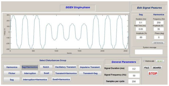
Figure 5.
Graphical interface of signal generator SIGEN.
The processes of SIGEN were performed to complete the effective generation of electric signals, as follows:
- First, electrical input signals were defined and the user set their parameters.
- Second, signals according to these specifications were built.
- Finally, the synthesized signals could be sent either to a file or a data acquisition board (DAQ).
SIGEN was designed following the guidelines described in the IEEE-1159 standard for monitoring electric power quality [57].
All the signals had in common the following fundamental specifications: Voltage = 230 V RMS (root mean square), frequency = 50 Hz, duration = 0.2 s, sampling frequency = 12.8 kHz, total cycles = 10, total samples = 2560. Stationary and/or transient disturbances, as well as white Gaussian noise, were added to this fundamental signal. The levels of added noise were characterized by the signal-to-noise (SNR) ratio of 20 dB, 30 dB, 40 dB, and 50 dB. For each noise level and each PQD category, 100 signals were generated through SIGEN by varying all the parameters. This set had a total of 5600 simulated signals, 1400 for each noise level involving all categories (13 types of the PQDs plus one pure sinusoidal signal). These signal sets transformed in the dataset intended to verify the classification performance, as will be seen next.
Another set of signals was needed for the feature selection stage. It included 560 simulated signals (40 signals 14 PQD categories) with random SNR between 20 dB and 50 dB.
6.2. Training/Testing and Validation Datasets
Once statistical features were computed based on the ST matrix, datasets were created. A first dataset contained data (samples features) and it was used as input of the K-NN-based fast validation tool for optimal feature selection (see Section 3.1 and Section 3.2).
As concluded in Section 3, the choice of either of the selected optimization algorithms (GA and CSO) allowed obtaining a feature set which comprised only five features. Thus, for each of the four specific noise levels considered, the second type of dataset containing data (samples features) was used to fit the different proposed classification models. This training dataset was partitioned into train/test datasets like 80/20%, respectively. Then, while the test dataset was kept aside, the train set split again into the actual train dataset (80% again) and the validation set (the remaining 20%). Data for each subset was randomly selected. This cross-validation procedure iteratively trained and validated the models on these sets, avoiding overfitting. In this study, a 10-folds cross-validation method was used to evaluate the performance of the proposed classifiers.
It must be noted that the mentioned training dataset was different to that one used in the previous feature selection stage. This ensured that no observations that were a part of the feature selection task were a part of the classification task.
6.3. PQDs’ Classes
The following 14 classes were tested and labelled as: Harmonic (C1), Flicker (C2), Sags (C3), Sags and harmonic (C4), Interruption (C5), Interruption and harmonic (C6), Notch (C7), Swells (C8), Swells and harmonic (C9), Oscillatory transient (C10), Oscillatory transient and harmonic (C11), Oscillatory transient and sag (C12), Impulsive transient (C13), and pure sinusoidal signal (C14). In Table 2 the simulated PQDs waveforms are depicted.
Table 2.
Synthetized PQDs’ waveforms.
7. Results and Performance Comparison
Depending on the optimization and pattern recognition approach selected, five hybrid classification methods were considered: CSO&QSVM (quadratic SVM), CSO&WK-NN (weighted K-NN), GA&FTree (fine tree), GA&ETree (ensemble tree), and GA&CSVM (cubic SVM). In Table 3, the classification accuracy on training dataset under different noise conditions of the proposed models are listed.
Table 3.
Recognition accuracy comparison between proposed methods under noisy conditions.
The best results of classification accuracy were obtained using CSO&QSVM in any noise conditions. The results for 30 dB SNR and above had high classification accuracy for both CSO&QSVM and CSO&WK-NN, and the rest of the models had acceptable values. In high noisy conditions (20 dB), the accuracy was satisfactory only for CSO&QSVM. The values obtained applying the rest of the methods were lower and required the next analysis with separate PQDs for a better interpretation of the results.
In order to evaluate noise immunity under different accuracy requirements, single-class test datasets (each with data of a unique class) were subjected to the trained classifiers separately. The noise threshold (minimum SNR value) for each class was determined through a trial-and-error method, by applying the principle of keeping SNR value as low as possible while maintaining the targeted classification accuracy. Thus, if the classification accuracy on an initial single-class dataset was, for example, lower than 80%, a new dataset with higher SNR value was generated and tested. The iterative procedure was stopped when the pretended accuracy was achieved. In Table 4, a comparison of minimum SNR values using these methods for different accuracy rates and distinct PQDs classes is presented. In each specific case, the maximum level of noise allowing the pretended accuracy rate (80%, 90%, and 100%) is shown. In the last row, the overall SNR average threshold value of each column is determined. This value was just an estimation of the noise immunity for a pretended accuracy rate in the separate classification process.
Table 4.
Comparison of noise threshold (SNR minimum) for classification accuracy of the models proposed.
From Table 4 it can be seen that the GA-based models offered good SNR values for most PQDs, often even better than those resulting from CSO algorithm, especially when dealing with single events. However, none of the suggested GA-based models was capable to classify properly the multiple interruption plus harmonic disturbances. In the same terms of working with five optimal features, both GA&FTree and GA&ETree also misclassified swell plus harmonic events and GA&CSVM could not resolve notches and harmonics disturbances. This lack of identification of a separated PQDs could justify the modest results obtained by GA-based models in Table 3. On the contrary, the proposed CSO-based models achieved good individual noise rates for a separate classification of classes according to different accuracy targets. As a result, both CSO&QSVM and CSO&WK-NN methods presented an overall SNR average threshold under 20 dB, specifically 18.57 dB and 19.54 dB, respectively. When both QSVM and WK-NN classifiers acted on single-class datasets, this slightly lower SNR value in the CSO&QSVM method suggested a better performance with regard to noise immunity. But this behavior in high noisy conditions was not only valid for single-class datasets, but also for the complete dataset. As shown above, in Table 3, CSO&QSVM obtained the best results also with the complete training dataset.
On the other hand, in Table 5, performances of the best-proposed CSO-QSVM method are compared to those of other classification methods already reported in the literature. It can be seen that some methods reported information of accuracy with noise levels (SNR) up to 50 dB [37,58], 40 dB [27], and 30 dB [42]. Others [17,59,60], although reaching 20 dB, had low accuracy. It is remarkable the high impact of noise in the accuracy of the wavelet-based approaches [37,60]. The remaining works presented acceptable accuracy [15,38,39,41,43] but none was capable to deal with 13 PQDs as the actual proposal did. Only [15] achieved similar performances than those of the proposed CSO-QSVM approach. That studied 12 kinds of single and multiple PQDs through the use of improved principal component analysis (IPCA) and 1-dimensional convolution neural network (1-D-CNN) and achieved an overall accuracy of 99.76% and 99.85% for 20 dB and 50 dB, respectively. That classifier needed six features, distinct from the optimal feature set proposed in this work, which was composed of only five of them.
Table 5.
Performance comparison of different methods.
Table 5 also displays a comparative in terms of feature dimension in each reported approach. The ST-based probabilistic neural network (PNN) approach [59] accepted a set with four features but only dealt with nine PQDs, while PNN based on wavelet [60] was treated with 14 PQDs but with poor noise immunity as indicated by its accuracy rates. This comparative study shows that the proposed CSO-QSVM model, at last, equaled the better results of classification accuracy obtained in the literature, but using only five features per sample and dealing with 13 PQDs classes. These results, together with the comparison between alternative proposals (Table 3) and the detailed analysis of noise immunity (Table 4), constitute the main contributions of this paper.
Although the present work dealt with simulated signals, the results were so good that they could be extrapolated when applied to experimental data. In such a case, a comparative with those studies based on real signals could be applied properly.
As a future extension, an experimental setup would be used to test the effectiveness of the proposed hybrid methods under common real-time working conditions. Emulated PQ incidence on distribution networks could be modelled by low-cost hardware prototyping and software components.
8. Conclusions
The motivation for this work stemmed from challenges facing the electrical systems and equipment in determining optimal, cost-effective, and efficient power quality management. In this way, this paper addressed the optimal hybrid classification methods based on machine learning approaches for meeting detection, identification, and classification of simulated PQDs. Specifically, ST was selected for detection and feature extraction of PQDs, and, following the trend nowadays to further optimize the recognition approach, several optimization algorithms were tested for optimal feature selection. At this step, this work underlined the GA and CSO algorithms since they achieved the best results. The resulting optimal feature sets were fed to several classifiers, highlighting among them the QSVM, CSVM, FTree, ETree, and WK-NN approaches for showing improved performance.
The GA optimization algorithm associated with the FTree, ETree, and CSVM approaches could not classify properly all PQDs under the conditions established in this analysis. However, the results obtained through these approaches were very promising and showed the great potential of these kinds of models when dealing with a certain group of PQDs.
Alternatively, CSO-based methods including CSO-QSVM and CSO-WK-NN achieved high classification accuracy under noisy conditions. A thorough comparative assessment in terms of noise immunity and classification accuracy led us to conclude that the proficiency of CSO-QSVM method is slightly better than CSO-WK-NN method.
It can also be noted that the results found seemed to confirm the current trend by which, despite the optimization based on GA algorithms being highlighted by their efficiency, GA-based methodologies are progressively being replaced by the swarm optimization algorithms.
Finally, performances of CSO-QSVM method were compared to those of other classification methods already reported in the literature, concluding that the proposed method achieved a higher degree of efficiency than most of them, and, based on the results, it may work well under high noise background in practical applications.
Author Contributions
J.C.B.-R. conceived and developed the idea of this research, designed the whole structure of the comparative study, and wrote the paper; F.J.T. generated the data, performed the simulations, and contributed to the methodology; M.D.B. provided the theoretical background of the proposed methodology and contributed to it. All authors have read and agreed to the published version of the manuscript.
Funding
This research was funded by the Universidad de Sevilla (VI Plan Propio de Investigación y Transferencia) under grant 2020/00000596.
Conflicts of Interest
The authors declare no conflict of interest.
Appendix A
The continuous Stockwell transform (ST) [1] of a signal x(t) was originally described as
i.e., a phase factor acting on a continuous wavelet transform (CWT)
where τ is a time displacement factor, d is a frequency-scale dilation factor, and is a specific mother wavelet that includes the frequency-modulated Gaussian window
Instead, in this paper, the STFT pathway to address the ST definition was preferred,
From this approach, ST can be written as
where is the Gaussian window function similar to that proposed by Gabor (1946), but now also introducing the aforementioned added frequency dependence
where the inverse of the frequency represents the window width.
From either of the two viewpoints, the complete ST definition can be written as
and also can be represented in terms of its relationship with FT and related spectrum X(f) of x(t)
As is well known, the way to recover the original signal from continuous ST is expensive in terms of data storage due to oversampling. This sampled version of the ST permits calculating the widely used ST complex matrix that is obtained as (τ → jT, f → n/NT)
where T denotes the sampling interval, N is the total number of sample points, and both and result after discrete fast Fourier transform (FFT), respectively, on the PQ disturbance signal x(t) and the Gaussian window function :
where j, k, m, and n are integers in the range of 0 to N − 1.
The result of discrete ST is a 2D time-frequency matrix that is represented as
where is the amplitude and is the phase. Each column contains the frequency components present in the signal at a particular time. Each row displays the magnitude of a particular frequency with time varying from 0 to N − 1 samples.
References
- Stockwell, R.; Mansinha, L.; Lowe, R. Localization of the complex spectrum: The S transform. IEEE Trans. Signal Process. 1996, 44, 998–1001. [Google Scholar] [CrossRef]
- Borras, M.D.; Bravo, J.C.; Montano, J.C. Disturbance Ratio for Optimal Multi-Event Classification in Power Distribution Networks. IEEE Trans. Ind. Electron. 2016, 63, 3117–3124. [Google Scholar] [CrossRef]
- Bravo, J.C.; Borras, M.D.; Torres, F.J. Development of a smart wavelet-based power quality monitoring system. In Proceedings of the 2018 International Conference on Smart Energy Systems and Technologies (SEST), Seville, Spain, 10–12 September 2018; pp. 1–6. [Google Scholar]
- Borras, M.-D.; Montano, J.-C.; Castilla, M.; López, A.; Gutierrez, J.; Bravo, J.-C. Voltage index for stationary and transient states. In Proceedings of the Mediterranean Electrotechnical Conference (MELECON), Valletta, Malta, 26–28 April 2010; pp. 679–684. [Google Scholar]
- Sahani, M.; Dash, P. FPGA-Based Online Power Quality Disturbances Monitoring Using Reduced-Sample HHT and Class-Specific Weighted RVFLN. IEEE Trans. Ind. Inform. 2019, 15, 4614–4623. [Google Scholar] [CrossRef]
- Afroni, M.J.; Sutanto, D.; Stirling, D. Analysis of Nonstationary Power-Quality Waveforms Using Iterative Hilbert Huang Transform and SAX Algorithm. IEEE Trans. Power Deliv. 2013, 28, 2134–2144. [Google Scholar] [CrossRef]
- Xi, Y.; Li, Z.; Zeng, X.; Tang, X.; Liu, Q.; Xiao, H. Detection of power quality disturbances using an adaptive process noise covariance Kalman filter. Digit. Signal Process. 2018, 76, 34–49. [Google Scholar] [CrossRef]
- Nie, X. Detection of Grid Voltage Fundamental and Harmonic Components Using Kalman Filter Based on Dynamic Tracking Model. IEEE Trans. Ind. Electron. 2020, 67, 1191–1200. [Google Scholar] [CrossRef]
- He, S.; Zhang, M.; Tian, W.; Zhang, J.; Ding, F. A Parameterization Power Data Compress Using Strong Trace Filter and Dynamics. IEEE Trans. Instrum. Meas. 2015, 64. [Google Scholar] [CrossRef]
- Manikandan, M.S.; Samantaray, S.R.; Kamwa, I. Detection and Classification of Power Quality Disturbances Using Sparse Signal Decomposition on Hybrid Dictionaries. IEEE Trans. Instrum. Meas. 2014, 64, 27–38. [Google Scholar] [CrossRef]
- Cho, S.-H.; Jang, G.; Kwon, S.-H. Time-Frequency Analysis of Power-Quality Disturbances via the Gabor–Wigner Transform. IEEE Trans. Power Deliv. 2009, 25, 494–499. [Google Scholar] [CrossRef]
- Lopez-Ramirez, M.; Ledesma-Carrillo, L.M.; Cabal-Yepez, E.; Rodriguez-Donate, C.; Miranda-Vidales, H.; Garcia-Perez, A. EMD-Based Feature Extraction for Power Quality Disturbance Classification Using Moments. Energies 2016, 9, 565. [Google Scholar] [CrossRef]
- Camarena-Martinez, D.; Valtierra-Rodriguez, M.; Perez-Ramirez, C.A.; Amezquita-Sanchez, J.P.; Romero-Troncoso, R.D.J.; Garcia-Perez, A. Novel Downsampling Empirical Mode Decomposition Approach for Power Quality Analysis. IEEE Trans. Ind. Electron. 2015, 63, 2369–2378. [Google Scholar] [CrossRef]
- Wu, X.; Kumar, V.; Ross Quinlan, J.; Ghosh, J.; Yang, Q.; Motoda, H.; McLachlan, G.J.; Ng, A.; Liu, B.; Yu, P.S.; et al. Top 10 algorithms in data mining. Knowl. Inf. Syst. 2008, 14, 1–37. [Google Scholar] [CrossRef]
- Shen, Y.; Abubakar, M.; Liu, H.; Hussain, F. Power Quality Disturbance Monitoring and Classification Based on Improved PCA and Convolution Neural Network for Wind-Grid Distribution Systems. Energies 2019, 12, 1280. [Google Scholar] [CrossRef]
- Erişti, H.; Yıldırım, Ö.; Erişti, B.; Demir, Y. Optimal feature selection for classification of the power quality events using wavelet transform and least squares support vector machines. Int. J. Electr. Power Energy Syst. 2013, 49, 95–103. [Google Scholar] [CrossRef]
- Huang, N.; Peng, H.; Cai, G.; Chen, J. Power Quality Disturbances Feature Selection and Recognition Using Optimal Multi-Resolution Fast S-Transform and CART Algorithm. Energies 2016, 9, 927. [Google Scholar] [CrossRef]
- Moon, S.-K.; Kim, J.-O.; Kim, C. Multi-Labeled Recognition of Distribution System Conditions by a Waveform Feature Learning Model. Energies 2019, 12, 1115. [Google Scholar] [CrossRef]
- Huang, N.; Lu, G.; Cai, G.; Xu, D.; Xu, J.; Li, F.; Zhang, L. Feature Selection of Power Quality Disturbance Signals with an Entropy-Importance-Based Random Forest. Entropy 2016, 18, 44. [Google Scholar] [CrossRef]
- Jamali, S.; Farsa, A.R.; Ghaffarzadeh, N. Identification of optimal features for fast and accurate classification of power quality disturbances. Meas. J. Int. Meas. Confed. 2018, 116, 565–574. [Google Scholar] [CrossRef]
- Singh, U.; Singh, S.N. Optimal Feature Selection via NSGA-II for Power Quality Disturbances Classification. IEEE Trans. Ind. Inform. 2017, 14, 2994–3002. [Google Scholar] [CrossRef]
- Ray, P.K.; Mohanty, S.R.; Kishor, N.; Catalão, J.P. Optimal Feature and Decision Tree-Based Classification of Power Quality Disturbances in Distributed Generation Systems. IEEE Trans. Sustain. Energy 2013, 5, 200–208. [Google Scholar] [CrossRef]
- Dehini, R.; Sefiane, S. Power quality and cost improvement by passive power filters synthesis using ant colony algorithm. J. Theor. Appl. Inf. Technol. 2011, 23, 70–79. [Google Scholar]
- Singh, U.; Singh, S.N. A new optimal feature selection scheme for classification of power quality disturbances based on ant colony framework. Appl. Soft Comput. 2019, 74, 216–225. [Google Scholar] [CrossRef]
- Wang, J.; Xu, Z.; Che, Y. Power Quality Disturbance Classification Based on DWT and Multilayer Perceptron Extreme Learning Machine. Appl. Sci. 2019, 9, 2315. [Google Scholar] [CrossRef]
- Chen, Z.; Han, X.; Fan, C.; Zheng, T.; Mei, S. A Two-Stage Feature Selection Method for Power System Transient Stability Status Prediction. Energies 2019, 12, 689. [Google Scholar] [CrossRef]
- Huang, N.; Zhang, S.; Cai, G.; Xu, D. Power Quality Disturbances Recognition Based on a Multiresolution Generalized S-Transform and a PSO-Improved Decision Tree. Energies 2015, 8, 549–572. [Google Scholar] [CrossRef]
- Vidhya, S.; Kamaraj, V. Particle swarm optimized extreme learning machine for feature classification in power quality data mining. Automatika 2017, 58, 487–494. [Google Scholar] [CrossRef]
- Cheng, R.; Jin, Y. A competitive swarm optimizer for large scale optimization. IEEE Trans. Cybern. 2014, 45, 191–204. [Google Scholar] [CrossRef]
- Gu, S.; Cheng, R.; Jin, Y. Feature selection for high-dimensional classification using a competitive swarm optimizer. Soft Comput. 2018, 22, 811–822. [Google Scholar] [CrossRef]
- Niu, B.; Yang, X.; Wang, H. Feature Selection Using a Reinforcement-Behaved Brain Storm Optimization. In Intelligent Computing Methodologies; Huang, D.-S., Huang, Z.-K., Hussain, A., Eds.; Springer International Publishing: Cham, Switzerland, 2019; Volume 11645, pp. 672–681. [Google Scholar]
- Sharaf, A.M.; El-Gammal, A.A.A. A discrete particle swarm optimization technique (DPSO) for power filter design. In Proceedings of the 2009 4th International Design and Test Workshop (IDT), Riyadh, Saudi Arabia, 15–17 November 2009. [Google Scholar] [CrossRef]
- Zhao, L.; Long, Y. An Improved PSO Algorithm for the Classification of Multiple Power Quality Disturbances. J. Inf. Process. Syst. 2019, 15, 116–126. [Google Scholar] [CrossRef]
- De Yong, D.; Bhowmik, S.; Magnago, F. Optimized Complex Power Quality Classifier Using One vs. Rest Support Vector Machines. Energy Power Eng. 2017, 9, 568–587. [Google Scholar] [CrossRef][Green Version]
- Janik, P.; Lobos, T. Automated Classification of Power-Quality Disturbances Using SVM and RBF Networks. IEEE Trans. Power Deliv. 2006, 21, 1663–1669. [Google Scholar] [CrossRef]
- Hajian, M.; Foroud, A.A. A new hybrid pattern recognition scheme for automatic discrimination of power quality disturbances. Measurement 2014, 51, 265–280. [Google Scholar] [CrossRef]
- Thirumala, K.; Pal, S.; Jain, T.; Umarikar, A.C. A classification method for multiple power quality disturbances using EWT based adaptive filtering and multiclass SVM. Neurocomputing 2019, 334, 265–274. [Google Scholar] [CrossRef]
- Li, J.; Teng, Z.; Tang, Q.; Song, J. Detection and Classification of Power Quality Disturbances Using Double Resolution S-Transform and DAG-SVMs. IEEE Trans. Instrum. Meas. 2016, 65, 2302–2312. [Google Scholar] [CrossRef]
- Noh, F.H.M.; Rahman, M.A.; Yaakub, M.F. Performance of Modified S-Transform for Power Quality Disturbance Detection and Classification. Telkomnika 2017, 15, 1520–1529. [Google Scholar]
- Zhong, T.; Zhang, S.; Cai, G.; Huang, N. Power-Quality disturbance recognition based on time-Frequency analysis and decision tree. IET Gener. Transm. Distrib. 2018, 12, 4153–4162. [Google Scholar] [CrossRef]
- Alqam, S.J.; Zaro, F.R. Power Quality Detection and Classification Using S-Transform and Rule-Based Decision Tree. Int. J. Electr. Electron. Eng. Telecommun. 2019, 1–6. [Google Scholar] [CrossRef]
- Biswal, M.; Dash, P.K. Measurement and Classification of Simultaneous Power Signal Patterns With an S-Transform Variant and Fuzzy Decision Tree. IEEE Trans. Ind. Inform. 2012, 9, 1819–1827. [Google Scholar] [CrossRef]
- Mahela, O.P.; Shaik, A.G. Recognition of power quality disturbances using S-transform based ruled decision tree and fuzzy C-means clustering classifiers. Appl. Soft Comput. 2017, 59, 243–257. [Google Scholar] [CrossRef]
- Samantaray, S. Decision tree-Initialised fuzzy rule-Based approach for power quality events classification. IET Gener. Transm. Distrib. 2010, 4, 538. [Google Scholar] [CrossRef]
- Goldberg, D.E.; Holland, J.H. Genetic Algorithms and Machine Learning. Mach. Learn. 1988, 3, 95–99. [Google Scholar] [CrossRef]
- Siedlecki, W.; Sklansky, J. A note on genetic algorithms for large-scale feature selection. Pattern Recognit. Lett. 1989, 10, 335–347. [Google Scholar] [CrossRef]
- Kang, M.; Kim, J.; Wills, L.; Kim, J.-M. Time-Varying and Multiresolution Envelope Analysis and Discriminative Feature Analysis for Bearing Fault Diagnosis. IEEE Trans. Ind. Electron. 2015, 62, 7749–7761. [Google Scholar] [CrossRef]
- Fan, G.-F.; Guo, Y.-H.; Zheng, J.-M.; Hong, W.-C. Application of the Weighted K-Nearest Neighbor Algorithm for Short-Term Load Forecasting. Energies 2019, 12, 916. [Google Scholar] [CrossRef]
- Vapnik, V.N. The Nature of Statistical Learning Theory; Springer: Berlin/Heidelberg, Germany, 1995. [Google Scholar]
- Cortes, C.; Vapnik, V. Support-Vector networks. Mach. Learn. 1995, 20, 273–297. [Google Scholar] [CrossRef]
- Ozgonenel, O.; Yalcin, T.; Guney, I.; Kurt, Ü. A new classification for power quality events in distribution systems. Electr. Power Syst. Res. 2013, 95, 192–199. [Google Scholar] [CrossRef]
- De Yong, D.; Bhowmik, S.; Magnago, F. An effective Power Quality classifier using Wavelet Transform and Support Vector Machines. Expert Syst. Appl. 2015, 42, 6075–6081. [Google Scholar] [CrossRef]
- A Survey on Decision Tree Algorithms of Classification in Data Mining. Int. J. Sci. Res. 2016, 5, 2094–2097. [CrossRef]
- Breiman, L. Random Forests. Mach. Learn. 2001, 45, 5–32. [Google Scholar] [CrossRef]
- IEEE Power and Energy Society. IEEE Standard Definitions for the Measurement of Electric Power Quantities Under Sinusoidal, Nonsinusoidal, Balanced, or Unbalanced Conditions; IEEE Std 1459-2010 (Revision IEEE Std 1459-2000); IEEE: New York City, NY, USA, 2010; pp. 1–50. [Google Scholar]
- European Committee for Electrotechnical Standardization. Voltage Characteristics of Electricity Supplied by Public Distribution Networks; EN-50160 2011; Eur. Std: 2010; CENELEC: Brussels, Belgium, 2010. [Google Scholar]
- IEEE Power and Energy Society. IEEE Recommended Practice for Monitoring Electric Power Quality; IEEE Std 1159-2019 (Revision IEEE Std 1159-2009); IEEE: New York City, NY, USA, 2019; pp. 1–98. [Google Scholar]
- Kumar, R.; Singh, B.; Shahani, D.T.; Chandra, A.; Al-Haddad, K.; Garg, R. Recognition of Power-Quality Disturbances Using S-Transform-Based ANN Classifier and Rule-Based Decision Tree. IEEE Trans. Ind. Appl. 2014, 51, 1249–1258. [Google Scholar] [CrossRef]
- Wang, H.; Wang, P.; Liu, T. Power Quality Disturbance Classification Using the S-Transform and Probabilistic Neural Network. Energies 2017, 10, 107. [Google Scholar] [CrossRef]
- Khokhar, S.; Zin, A.A.M.; Memon, A.P.; Mokhtar, A.S. A new optimal feature selection algorithm for classification of power quality disturbances using discrete wavelet transform and probabilistic neural network. Measurement 2017, 95, 246–259. [Google Scholar] [CrossRef]


© 2020 by the authors. Licensee MDPI, Basel, Switzerland. This article is an open access article distributed under the terms and conditions of the Creative Commons Attribution (CC BY) license (http://creativecommons.org/licenses/by/4.0/).