Abstract
Modeling and control of proton-exchange membrane fuel cells (PEMFC) has become a very popular research topic lately due to the increasing use of renewable energy. Despite this fact, most of the work in the current literature only studies standard dynamical models without taking into consideration possible parasitics such as small gas flow perturbations that could be available in the system. This paper addresses this issue by elaborating on time-scale modeling of an augmented eighteenth-order PEMFC-reformer system via singular perturbation theory. The latter captures time scales that arise in the model due to the presence of small perturbations. Specifically, a novel and efficient algorithm that helps identify the presence of different time-scales is developed. In addition, the method converts an implicit singularly perturbed model into an explicit equivalent where the time-scales are evident. Using this algorithm, a complete singularly perturbed dynamic model of the augmented eighteenth-order PEMFC-reformer system is obtained. Modeling of the PEMFC-reformer system is followed by linear quadratic regulator (LQR) design for the individual time-scales present in the system.
1. Introduction
An increase in worldwide energy demand and the quest for sustainability have led to major investments in renewable resources. The latter are eco-friendly, generally reliable, and have lower operating costs. While there are several disadvantages associated with renewable sources such as vulnerability or the inability to generate power in large quantities, the consensus among researchers is that energy in the future will primarily be generated by renewable sources. One of the latter is the fuel cell. This source has become very popular due to a higher efficiency compared to other renewable sources, low maintenance costs, and ubiquity of hydrogen. Fuel cells have been widely used in industrial settings (e.g., factories) [1], residential units [2], and the automotive industry (e.g., electric vehicles) [3,4], and are also commonplace in smart grid ecosystems where they are used as supplementary renewable sources in microgrids [5,6]. A major enabler that has aided in hydrogen mobility, and subsequently in the widespread use of fuel cells, has been the investment in infrastructure by several countries in North America, Europe, and Asia [7,8]. Government statistics in these countries [8] show that demand for a hydrogen economy is increasing, hence possibly putting the fuel cell at the forefront of the clean energy revolution.
The device works by converting the chemical energy of hydrogen and oxygen into electricity through a pair of redox reactions [9]. In addition to electricity, the chemical reaction produces water and heat [9,10]. While the method of operation is standard for all varieties of fuel cells, they have distinct features such as different material composition, efficiency, and operating temperatures. Some of the most common types that are currently in use and also heavily researched are the proton-exchange membrane fuel cell (PEMFC) [9], the solid oxide fuel cell (SOFC) [11], and the phosphoric acid fuel cell (PAFC) [12].
It is worth noting that modeling and simulation play a critical role in fuel cell design. A high-fidelity model gives the designer the capability to modify parameters accordingly and use them in the final implementation, therefore leading to an optimal desired design. One such PEMFC model was originally developed in [9]. This model has been investigated in a variety of domains over the years. For example, in [13], the authors consider dynamic and controlled operation of a PEMFC integrated with a natural gas fuel processor system (FPS) and a catalytic burner (CB). Optimization is performed to generate the air and fuel flow intake setpoints to the fuel processor system for different load levels, and then linear quadratic regulator techniques are used to develop a controller to mitigate hydrogen starvation in the fuel cell. In [9], analysis and design of air flow controllers that prevent oxygen deprivation of the fuel cell stack as the current changes was presented. Improvements in transient oxygen regulation when the fuel processing system voltage was included in the model were demonstrated. A combined PEMFC-FPS model was studied in [14], where the authors used order-reduction techniques to show that similar controller performance can be obtained if the model size is reduced.
Unlike the work of [9] and other aforementioned references, this research differs in that an augmented singularly perturbed model of the PEMFC-FPS is obtained. While the latter has been defined in [14], it has not been studied in a singularly perturbed fashion. The technological context as well as the motivation behind this work lies in the fact that fuel cell systems can contain inherent parasitics such as small impedances or load perturbations. A standard dynamic model does not include such parasitics and that can lead to inaccuracies in simulations which, in turn, would affect the efficiency of the overall system design. Singular perturbation methods are typically used for such models and are very important from a practical aspect since they capture the model’s slow and fast dynamics, hence providing a more accurate model. Besides the singularly perturbed modeling of the fuel cell system, case studies of optimal controller design are presented. Namely, linear quadratic (LQ) controllers are designed for the individual time-scales to meet operational requirements. It is important to note that in this paper, the term “fuel cell system” strictly refers to a setup consisting of a PEMFC and an FPS and does not include additional components such as filters, converters, etc.
The contributions of this paper are threefold. First, the theory that enables one to convert an arbitrary linear system with two or more time-scales into a singularly perturbed model is developed. The algorithm leverages an ordered Schur decomposition that arranges the system’s eigenvalues along the main diagonal. Furthermore, the algorithm is computationally efficient, which is essential from a practical perspective (e.g., parametric studies). Next, the singularly perturbed model of the overall PEMFC-FPS is derived and formalized. Lastly, LQ controllers for each of the lower order models are designed so that the response meets operational requirements.
The paper is organized as follows. In Section 2, the preliminaries of PEMFCs and singularly perturbed systems are introduced. In Section 3, theoretical details on time-scale decoupling via the ordered Schur decomposition are presented. Section 4 covers the singularly perturbed modeling of the PEMFC-FPS, followed by Section 5 where LQ controller design is illustrated. The remaining sections, namely, Section 6 and Section 7, correspond to the Results and Discussion, and Conclusions, respectively.
2. Preliminaries
2.1. PEM Fuel Cells
The purpose of this subsection is to familiarize the reader with the PEMFC. For more details on the topic, the reader is referred to [9,10,13] and the references therein. A simplified fuel cell diagram is shown in Figure 1. The PEMFC contains an electrolyte (center unit in Figure 1), an anode, and a cathode. Hydrogen and oxygen gas are the primary fuels used in the redox chemical reaction. The products of the latter are energy, excess fuel (if any), water, and heat. Due to several advantages, such as no harmful gas emissions, light weight, small size, and low operating temperature, the PEMFC has become a very popular energy alternative.
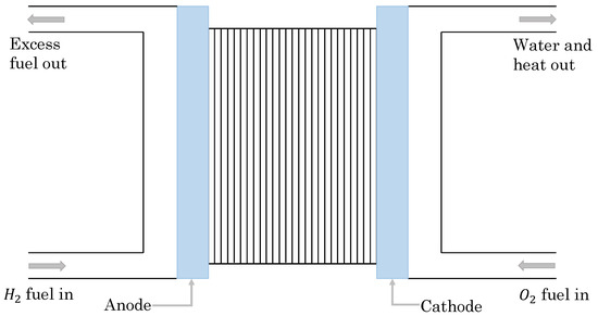
Figure 1.
Simplified diagram of a proton-exchange membrane fuel cells (PEMFC). The proton-exchange membrane is located between the anode and cathode.
The chemical reaction starts at the anode, where hydrogen fuel is processed and electrons are separated from protons on the surface of a catalyst. The electrons travel via a circuit to generate electricity while the protons pass through the membrane to the cathode of the cell. At the cathode, existing protons and electrons coming from the circuit are combined with oxygen to produce water, which together with heat are the only waste products. It is important to note that instead of oxygen gas in purified form, air can also be used as a fuel. An additional process at the electrode extracts oxygen from air which is then used in the chemical reaction.
The hydrogen gas going into the fuel cell on the other hand has to be in pure form. It can either be supplied from a dedicated tank or obtained from a fuel processing system (FPS) also known as a gas reformer. The FPS typically uses natural gas as raw material and produces hydrogen via a series of chemical reactions.
This research investigates the modeling and controller design of a PEMFC and FPS originally studied in [9]. Unlike in [9], this work explores the singularly perturbed modeling of the PEMFC-FPS augmented system. On that end, an overview of singular perturbation methods in control is provided in the following subsection to familiarize the reader with the theory.
2.2. Overview of Singularly Perturbed Methods in Control
While singular perturbation methods in control have been used extensively since the sixties [15], they are still an important research topic [16,17,18]. For a detailed treatment of singular perturbation methods, the reader is referred to [15,19,20,21] and the references therein.
A linear time-invariant (LTI) strictly proper singularly perturbed system in mathematical form is represented as
where and are the slow and fast state variables respectively, are the system control inputs, are the system measurements, and is the small singular perturbation parameter . In a real physical system, can represent parasitic capacitance in a circuit, moment of inertia in a mechanical system, etc. All the matrices in (1) are constant and of appropriate dimensions. Two time-scale LTI singularly perturbed systems have eigenvalues located in two disjoint groups: slow eigenvalues close to the imaginary axis and fast eigenvalues far from it. The following standard assumption is imposed [19].
Assumption 1.
Matrix is nonsingular.
When (a common strategy for order reduction), the following reduced-order system corresponding to the slow dynamics is obtained:
where
The approximated fast subsystem is [19]
where . According to the theory of singular perturbations [15,19], the approximation obtained in (2)–(4) satisfies
Hence, the smaller , the better the approximation. Furthermore, and are perturbation from the slow and fast eigenvalues of the original model, respectively.
Another effective method to obtain exact dynamic decoupling is by utilizing the transformation developed in [22]. Referred to as the Chang transformation, it diagonalizes the system by exposing the slow and fast dynamics. The transformation is given as follows.
A noticeable difference between the reduced-order slow model defined in (2)–(3) and the decoupled system (7) is that the measurement in (7) lacks an input while from (2) includes a term.
Matrices L and H are obtained by solving the following equations.
The reader can refer to [23,24,25] for methods on finding the solution of L and H.
3. Time-Scale Decoupling via the Ordered Schur Decomposition
This section serves as the basis for the singularly perturbed modeling of the PEMFC-FPS augmented system. Namely, the algorithm that achieves complete decoupling of an arbitrary singularly perturbed model is developed. This method is then applied in the following section. Theoretical techniques presented here were briefly introduced in [26]. This section contains a thorough explanation of the method.
3.1. Ordered Schur Transformation
As noted earlier, many real physical systems contain small parasitics when they are modeled. This forces parts of the system to operate in different time-scales. Quite often, it may be difficult to distinguish between the time-scales. Methods such as permutation matrices or other similarity transformations [19] have been proven successful to obtain a standard singularly perturbed form for two time-scale systems but it is challenging when additional time-scale dynamics are present.
In this paper, the aforementioned issue is addressed by developing a method that brings an implicit singularly perturbed system into its explicit form, where the perturbation parameters are either known or can be easily determined. is associated with the slowest state variable and is associated with the fastest, namely, .
Consider a general implicit multiple time-scale system without inputs, as shown in (10).
where is the state vector. To simplify the problem, an ordered Schur decomposition is employed to transform the model into a well-conditioned form. This is followed by the extraction of the perturbation parameter and sequential decoupling to obtain the individual time scales. The Schur decomposition is an efficient method used to find the system’s eigenvalues by utilizing the QR algorithm [27].
For a matrix , there exits a unitary matrix such that is upper quasi-triangular.
Matrix blocks can be or . blocks correspond to real eigenvalues while blocks correspond to complex eigenvalues.
The eigenvalues appearing along the diagonal of can be arbitrarily ordered. An additional transformation has to be employed to achieve desired reordering (descending) of the system matrix [27,28,29]. A transformation [30] can be found such that the unitary matrix T decomposes the system into the Schur form. Upon applying the ordered Schur algorithm, the dynamic Equation (10) takes the following form
where
Diagonal block matrices , , contain the system’s eigenvalues in descending order. are vectors each representing each time scale and are matrix blocks of appropriate dimensions. Note that blocks , , represent individual time-scales rather than individual eigenvalues.
3.2. Parameter Extraction and Time-Scale Decoupling
Prior to decoupling the transformed system, it is essential to convert it to an explicit singularly perturbed form by extracting the perturbation parameters from the system matrix. This is achieved by defining the perturbation parameters. For two time-scale stable systems with clearly separated eigenvalues (real or complex with small imaginary parts), is commonly evaluated as [31]. However, referring to examples such as the PEMFC-FPS under consideration, it can be inferred that the imaginary parts of the eigenvalues are indispensable for calculating the perturbation parameter. Hence, the latter is evaluated as the ratio of the magnitudes of the largest eigenvalue of the slowest time-scale with the smallest eigenvalue of the next fastest time-scale
Since the system is in ordered Schur form, the perturbation parameters can be easily evaluated using (14) and extracted to put the system into the explicit singularly perturbed form. The explicit multi-time-scale system now looks as follows:
where the elements of the system matrix have been scaled in accordance with parameter extraction.
The explicit system can now be decoupled into multiple distinct time-scale systems by successively applying the Chang transformation in (6).
To initiate the decoupling, the perturbation parameter is extracted from the fastest time-scale and (12) is rewritten as a standard two time-scale singularly perturbed form.
In (16), matrices and represent the last row of the system’s matrix in (13) with extracted. represents the fastest time-scale, while contains the rest of the matrix blocks which happen to be all zero in this case. and are matrices of appropriate dimensions containing the rest of the system matrix in (12).
Utilizing (6), the system in (16) is initially decoupled into two subsystems, where the fast subsystem represents the fastest time-scale available and the slow subsystem contains the rest of the time-scales.
As a reminder to the reader, matrices L and H satisfy (9). A modified Newton’s method developed in [25] follows.
The new slow subsystem (17a) is partitioned again, as in (19), where is now extracted from the second fastest time-scale.
The algorithm is applied sequentially till all the perturbation parameters have been extracted and the system is in explicit singularly perturbed form. The relation between the system in original coordinated and the new one is given as
where T is defined as and is
Matrix represents the linear transformation for each time-scale i. On the other hand, matrix is an augmentation of with an identity matrix I of appropriate dimensions so that its size is the same as T. Unlike in [31], the system matrix in ordered Schur form simplifies the computations. For a quasi-triangular system such as (12), in (16) is . Then, equations for the solution of matrices L and H in (9) simplify to the following.
An additional simplification comes due to the new system matrix structure.
Theorem 1.
Due to the structure of (15), matrix of the Chang transformation evaluates to a zero matrix.
Proof.
Upon applying the recursive algorithm (18), it is easy to show that matrix in (22a) evaluates to a zero matrix by solving the Sylvester equation for the first iteration
Matrix M is defined as and is full rank. Therefore, , which implies . Since and , then by induction, for all other iterations . This applies to matrix , for the remaining time-scales. □
In the absence of matrix L, (22b) then becomes just a Sylvester equation.
Likewise, transformation (6a) simplifies to (25). Note that the state variables in (25) are arbitrary.
After the process is repeated for all the N time-scales available in the system, the individual subsystems are then given as follows.
System (26) is now completely decoupled into a standard explicit singularly perturbed form. Note that if control is considered, the input matrix for each time-scale would be obtained sequentially in a similar fashion. The slow and fast input matrices for a two time-scale system are evaluated as and , respectively.
The overall process discussed in this section can be summarized as follows.
| Algorithm 1 Time-Scale Decoupling of Implicit Singularly Perturbed Systems |
|
4. Singularly Perturbed Modeling of the PEMFC-FPS
The general nonlinear models of the PEMFC and FPS systems studied in this paper were originally derived and used for controller design in [9]. The fuel cell considered in [9] has been used for research in the automotive industry and has a stack size of approximately 40 kW. Its operation temperature varies from 50 C to 100 C. The associated FPS is typically used for PEMFCs with stack size of 100 kW and is made up of a hydrodesulfurizer, a catalytic partial oxidation reactor, a water gas shift reactor, and a preferential oxidation reactor [9]. Original PEMFC and FPS models have been linearized around a nominal operation point, where the system net power is kW and oxygen excess ratio is [9]. Both linear and nonlinear model responses are compared in [9] and it is validated that the errors are insignificant.
This paper does not elaborate any further on the nonlinear systems but instead uses the linearized system for modeling and controller design. The reader is referred to [9,10] for additional details.
4.1. PEMFC and FPS Linear Model
Variables that are used in determining the model of the PEMFC fall into two main categories: masses of the gases that are used in the chemical reaction and the pressure of these gases. The state vector for the linear PEMFC model is defined as . Corresponding descriptions of state variables is provided in Table 1.

Table 1.
PEMFC nomenclature.
Likewise, for the FPS, masses and pressures of gases are essential for modeling. The state vector in this case is . Table 2 describes the state variables of the tenth order FPS model.
Table 2.
Fuel processing system nomenclature.
Using information from the PEMFC and FPS models, an augmented linear state-space model is created as in (27) [14].
State-space system in (27) can be written as follows:
where , , , and represent matrices in (27). Numerical values of , , , , , and are available in [9] and also included in Appendix A for reference. Note that the feedthrough matrix D is zero in both the PEMFC and FPS, therefore .
4.2. Singularly Perturbed Model of the PEMFC-FPS
The eigenvalues of the augmented system are key in determining the time-scale composition of the model. Figure 2 depicts graphically the sorted eigenvalues of the PEMFC-FPS. Recall from Section 3.2 that the magnitude of the eigenvalues is used to evaluate the singular perturbation parameter . Based on the distribution shown in Figure 2, a three time-scale model is chosen. The first nine modes represent the slow subsystem, the following six represent the second time-scale, and the last three constitute the fastest time-scale. Note that this decision is not necessarily strict.
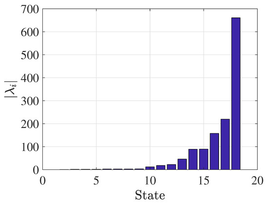
Figure 2.
Magnitude of the eigenvalues of the PEMFC-FPS (fuel processor system) augmented system. The reader can observe that the first nine eigenvalues are , the following six are , and the remaining are . Separation between clusters implies that three different time-scales are available.
At this point, the singular perturbation parameters of the three time-scale model can be calculated using (14). The magnitude of the largest eigenvalue of the slow subsystem is . The magnitude of the smallest eigenvalues of the second and third time-scales are and . Hence, , , and are as follows.
The singularly perturbed model then becomes
State variables belonging to each time-scale are presented in Table 3.
Table 3.
State variable distribution among time-scales.
After applying the algorithms developed in Section 3 to the original augmented PEMFC-FPS model in (27), the matrices that help form the singularly perturbed model (30) are obtained. The state matrix , control matrix , and output matrix are available in Appendix B. Linear mapping T represents the transformation from the original augmented model (27) to the ordered Schur model. It is also important to note that matrices and , specified in Appendix B, do not represent the state and control matrices in (30) because the singular perturbation parameters have not been extracted yet. To obtain model (27), and are simply multiplied by the of the corresponding time-scale.
Lastly, the Chang transformation [22] is applied sequentially to obtain a completely decoupled system (refer to Algorithm 1).
5. LQ Control System Design for the PEMFC-Reformer System
In this section, LQ controller design is demonstrated for the decoupled subsystems of the PEMFC-FPS model obtained in the previous section. Specifically, all three time-scales are considered independent models and LQ control is applied to each of them. An overview of LQ control is first presented followed by simulation results.
5.1. LQ Control Overview
In LQ control, our objective is to drive the state vector to the origin from any nonzero initial state [32]. If only state-feedback control is used and the closed-loop eigenvalues are assigned far inside the left half of the s-plane, the state will die out quickly but elements of the feedback gain can be high in magnitude, therefore requiring a high control cost. Alternatively, if the closed-loop eigenvalues are assigned closer to the imaginary axis, the rate of decay of will be slow and a small control action will be required. This trade-off between the state-vector and control action can be represented by the following cost function.
The LQ problem is then to find a control such that the cost function (31) is minimized. An important assumption here is that and . The solution to this infinite-horizon optimal control problem is a control input given by [32]
where the gain is given as and matrix P is the solution of the following algebraic Riccati equation [32].
The state vectors for each time-scale are given in Table 3.
5.2. Feedback Controller Design
Controller design starts with the decoupled PEMFC-FPS model presented in (27). Initially, the ordered Schur transformation is applied to obtain model (30) followed by sequential Chang transformation (6) to get a decoupled three time-scale model as follows.
In (34), , , and . The overall similarity transformation to arrive to (34) from original model (27) is , where is in itself two different linear transformations, namely, . Note that has the form given in (21).
The control input vector for system (34) now becomes as follows.
Note that it is important to convert the control input vector into the original coordinates of the system [33]. To do so, the transformation is used to put the system in coordinates, where represents the ordered Schur model. Another similarity transformation to get to the original coordinates is necessary, namely, . The control input them becomes
In the following subsection, the aforementioned principles are applied to the decoupled PEMFC-FPS model. It is worth noting that pairs and for all the state-space models considered are stabilizable and detectable, respectively.
5.3. LQ Control Simulation Results
LQ controller design in this section is based on requirements of an actual physical system as noted in [10]. Table 4 shows operating time specifications for different processes that occur in a PEFMC-reformer system. In this section, LQ controllers for one state in each time-scale are designed. Scaled reference step inputs are considered in each of the three cases. The selection of matrices Q and R in this section is based on parametric studies. This method ensures that (31) is minimized and requirements in Table 4 are met. An example of LQ control for various values of Q and R is shown in Figure 3 for . It is evident that different values of Q (shown as the trace of Q in this case) and R can have a significant impact on the controller’s response.
Table 4.
Fuel cell system operating time requirements.
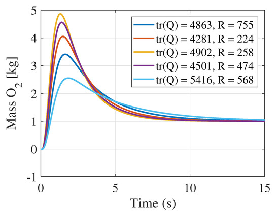
Figure 3.
Linear quadratic regulator (LQR) design for for various Q and R values.
Recall that the first subsystem corresponding to the slowest time-scale is a ninth-order model. For this case, only the mass of oxygen, namely is selected for control. From Table 4 (see [10]), it is observed that this process has a time constant of seconds. Ideally, for a satisfactory performance, it is preferred that the response settles in less than ten seconds. Likewise, a relatively small overshoot would be ideal so that the mass of oxygen in the chamber does damage the hardware. Figure 4 shows the response for a reference input set to 1 kg. The simulation is run for fifteen seconds. It can be observed that the settling time is around eight seconds (within the requirements). There is a noticeable overshoot but given the time duration, it does not pose any risks to the hardware. The values of the matrices Q and R used for this design are presented in (37).
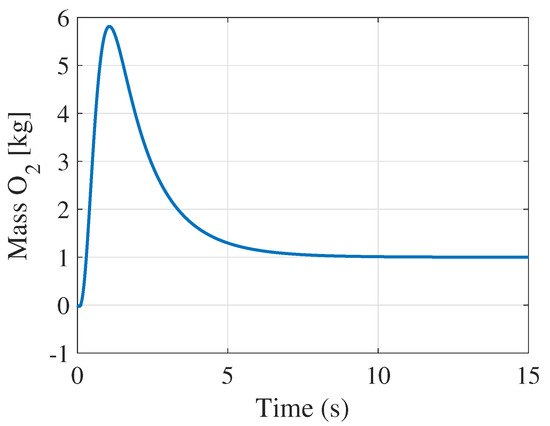
Figure 4.
LQR design simulation results for .
Figure 5 represents the second fastest subsystem. Specifically, the state variable corresponding to the pressure in the supply manifold has been used to demonstrate controller design. A reference input of 7 kPa has been used in the simulation. According to the requirements, the operational time for processes occurring in the manifold are of seconds. Therefore, the design entails a very short settling time and a small overshoot.
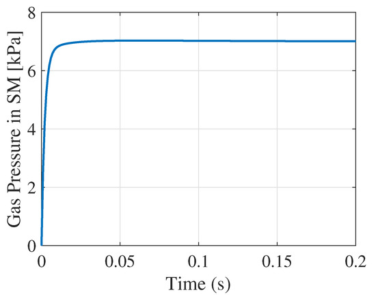
Figure 5.
LQR simulation results for .
Simulation results of the design are presented in Figure 5. It is clear that this design provides a short rise time, a very minimal settling time which falls within the requirements, and no overshoot.
The parameters for this desired design are given as follows.
Lastly, response for the fastest subsystem is shown in Figure 6. In the latter, results for the state corresponding to the mass of nitrogen () are shown, for a reference input of 0.5 kg. The simulation is run for seconds as the reader can observe. It is clear from Figure 6 that the mass of goes to the desired setpoint in a very short period of time. In addition, the design ensures a short rise time and no overshoot.
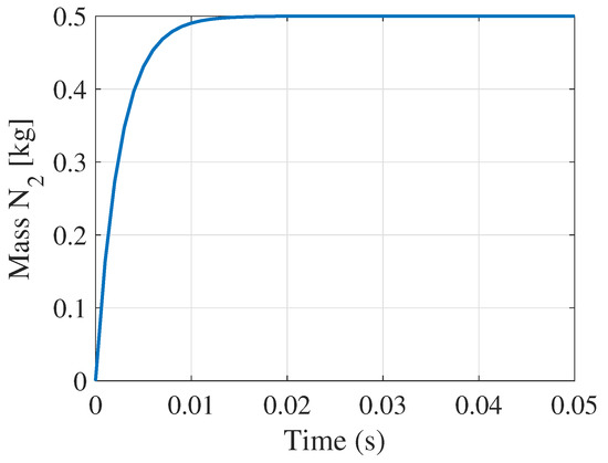
Figure 6.
LQR design simulation results for .
6. Discussion of Results
Results of this research can be divided into two main parts:
- Introduction of an algorithm that converts implicit singularly perturbed systems into explicit ones.
- Singularly perturbed modeling of the PEMFC-FPS augmented model followed by LQ controller design.
6.1. From Implicit to Explicit Singularly Perturbed Systems
The theoretical basis behind this research lies in the development of an algorithm that converts a linear system with known two or more time-scales (this could be determined from the eigenvalue distribution for example) into a singularly perturbed model. The algorithm relies on an ordered Schur decomposition. Singular perturbation parameters are determined via the ratio of the eigenvalues, and their extraction leads to a final singularly perturbed form. Then, exact decoupling of the obtained singularly perturbed system is sequentially performed.
The developed algorithm is an efficient method that help obtain an explicit form where the time-scales are clearly defined. While there are different methods to put an implicit singularly perturbed system into its explicit equivalent (for example, using permutation matrices), our method offers more flexibility. For instance, if the model is very large scale, using permutation matrices may not be feasible and it could be computationally expensive.
6.2. Singularly Perturbed Modeling of the PEMFC-FPS and Controller Design
The main novelty of this research lies in the formulation of the singularly perturbed model of the PEMFC-FPS. Starting with an augmented PEMFC-FPS model, the theoretical basis to obtain a model that is completely decoupled into different time-scales was presented. The enablers behind the modeling are the eigenvalues of the system. Large magnitude differences among the eigenvalues show that the augmented system consists of multiple time-scales, and since singular perturbation theory is commonly used to study such systems, it was applied to (27).
Using this method, the explicit singularly perturbed model (30) was obtained. The latter model was decoupled and controllers were designed for each sub-subsystem. Results showed that a performance within operational requirements can be attained.
6.3. Real-World Implications
Modeling and simulation are key tools used for a successful fuel cell system design. In this paper, a modeling methodology was initially developed by using singular perturbation techniques. The method helps obtain an explicit singularly perturbed model and also offer a way to decouple the model into individual time-scales which can be used separately to design controllers. Having a complete model and efficient algorithms is very important not only because it enables the designer to rigorously analyze the system but also because it helps alleviate computational burdens if, for example, parametric studies or Monte Carlo runs are considered.
7. Conclusions
A lack of PEMFC-FPS time-scale modeling served as motivation for this research. Initially, the theoretical basis that enables the designer convert a linear model with multiple time-scales into an explicit singular perturbation model was introduced. These techniques were applied to a popular augmented PEMFC-FPS model and it was shown that it can be represented as a three time-scale singularly perturbed model. The latter was then decoupled into individual submodels, each corresponding to a different time-scale, and LQ control was applied in each case. The methods developed in this paper capture all the dynamics present in the system including small parasitics. From a practical standpoint, the work presented here is indispensable to the designer since, in addition to a complete model, the efficient algorithm helps decouple the full-order model into individual time-scales for separate analysis such as controller design, as it was shown via case studies.
Author Contributions
Conceptualization, methodology, investigation, writing–original draft preparation, and software, K.K.; conceptualization, validation, formal analysis, investigation, and writing–review and editing, N.Z. All authors have read and agreed to the published version of the manuscript.
Funding
This research received no external funding.
Conflicts of Interest
The authors declare no conflict of interest.
Abbreviations
The following abbreviations are used in this manuscript (alphabetical order):
| CB | Catalytic burner |
| FPS | Fuel processing system |
| LQ | Linear quadratic |
| PAFC | Phosphoric acid fuel cell |
| PEMFC | Proton exchange membrane fuel cell |
| SOFC | Solid oxide fuel cell |
Appendix A. Linear Model Matrices
Appendix A.1. PEMFC Model State-Space Matrices
The corresponding control and output matrices are
Appendix A.2. Reformer Model State-Space Matrices
The corresponding control and output matrices are
Appendix B. Singularly Perturbed Model Matrices
Matrices , , and after the ordered Schur transformation.
where
References
- Casas, Y.; Dewulf, J.; Arteaga-Pérez, L.E.; Morales, M.; Van Langenhove, H.; Rosa, E. Integration of Solid Oxide Fuel Cell in a sugar–ethanol factory: Analysis of the efficiency and the environmental profile of the products. J. Clean. Prod. 2011, 19, 1395–1404. [Google Scholar] [CrossRef]
- Bizon, N.; Mazare, A.G.; Ionescu, L.M.; Enescu, F.M. Optimization of the proton exchange membrane fuel cell hybrid power system for residential buildings. Energy Convers. Manag. 2018, 163, 22–37. [Google Scholar]
- Serpi, A.; Porru, M. Modelling and Design of Real-Time Energy Management Systems for Fuel Cell/Battery Electric Vehicles. Energies 2019, 12, 4260. [Google Scholar] [CrossRef]
- Lee, D.-Y.; Elgowainy, A.; Vijayagopal, R. Well-to-wheel environmental implications of fuel economy targets for hydrogen fuel cell electric buses in the United States. Energy Policy 2019, 128, 565–583. [Google Scholar]
- Qazi, S.H.; Mustafa, M.W.; Sultana, U.; Mirjat, N.H.; Soomro, S.A.; Rasheed, N. Regulation of Voltage and Frequency in Solid Oxide Fuel Cell-Based Autonomous Microgrids Using the Whales Optimisation Algorithm. Energies 2018, 11, 1318. [Google Scholar]
- Brunaccini, G.; Sergi, F.; Aloisio, D.; Randazzo, N.; Ferraro, M.; Antonucci, V. Fuel cells hybrid systems for resilient microgrids. Int. J. Hydrogen Energy 2019, 44, 21162–21173. [Google Scholar] [CrossRef]
- Viesi, D.; Crema, L.; Testi, M. The Italian hydrogen mobility scenario implementing the European directive on alternative fuels infrastructure (DAFI 2014/94/EU). Int. J. Hydrogen Energy 2017, 42, 27354–27373. [Google Scholar] [CrossRef]
- Tlili, O.; Mansila, C.; Frimat, D.; Perez, Y. Hydrogen market penetration feasibility assessment: Mobility and natural gas markets in the US, Europe, China and Japan. Int. J. Hydrogen Energy 2019, 44, 16048–16068. [Google Scholar] [CrossRef]
- Pukrushpan, J.T.; Stefanopoulou, A.G.; Peng, H. Control of Fuel Cell Power Systems: Principles, Modeling, Analysis and Feedback Design, 1st ed.; Springer: New York, NY, USA, 2010. [Google Scholar]
- Pukrushpan, J.T.; Stefanopoulou, A.G.; Peng, H. Control of fuel cell breathing. IEEE Control Syst. Mag. 2004, 24, 30–46. [Google Scholar]
- Minh, N.Q. Solid oxide fuel cell technology—Features and applications. Solid State Ion. 2004, 174, 271–277. [Google Scholar] [CrossRef]
- Fuller, T.F.; Gallagher, K.G. Phosphoric acid fuel cells. In Materials for Fuel Cells, 1st ed.; Woodhead Publishing Series in Electronic and Optical Materials; Gasik, M., Ed.; Woodhead Publishing: Cambridge, UK, 2008; pp. 209–247. [Google Scholar]
- Tsourapas, V.; Stefanopoulou, A.G.; Sun, J. Model-based control of an integrated fuel cell and fuel processor with exhaust heat recirculation. IEEE Trans. Control Syst. Technol. 2007, 15, 233–245. [Google Scholar]
- Kodra, K.; Gajic, Z. Order reduction via balancing and suboptimal control of a fuel cell-reformer system. Int. J. Hydrogen Energy 2014, 39, 2215–2223. [Google Scholar]
- Kokotovic, P.V.; O’Malley, R.E.; Sannuti, P. Singular perturbations and order reduction in control theory—An overview. Automatica 1976, 12, 123–132. [Google Scholar] [CrossRef]
- Kodra, K.; Gajic, Z. Optimal control for a new class of singularly perturbed linear systems. Automatica 2017, 81, 203–208. [Google Scholar] [CrossRef]
- Kodra, K.; Skataric, M.; Gajic, Z. Finding Hankel singular values for singularly perturbed linear continuous-time systems. IET Control Theory A 2017, 11, 1063–1069. [Google Scholar] [CrossRef]
- Meng, X.; Wang, Q.; Zhou, N.; Xiao, S.; Chi, Y. Multi-Time Scale Model Order Reduction and Stability Consistency Certification of Inverter-Interfaced DG System in AC Microgrid. Energies 2018, 11, 254. [Google Scholar] [CrossRef]
- Kokotovic, P.; Khalil, H.; O’Reilly, J. Singular Perturbation Methods in Control: Analysis and Design, 2nd ed.; SIAM Press: Philadelphia, PA, USA, 1999. [Google Scholar]
- Naidu, D.S.; Calise, A.J. Singular perturbations and time scales in guidance and control of aerospace systems: A survey. J. Guid. Control Dyn. 2001, 24, 1057–1078. [Google Scholar] [CrossRef]
- Gajic, Z.; Lelic, M. Improvement of system order reduction via balancing using the method of singular perturbations. Automatica 2001, 37, 1859–1865. [Google Scholar] [CrossRef]
- Chang, K.W. Singular perturbations of a general boundary value problem. SIAM J. Math. Anal. 1972, 3, 520–526. [Google Scholar] [CrossRef]
- Gajic, Z.; Lim, M.-T. Optimal Control of Singularly Perturbed Linear Systems and Applications: High Accuracy Techniques, 1st ed.; CRC Press: Boca Raton, MA, USA, 2001. [Google Scholar]
- Kecman, V.; Bingulac, S.; Gajic, Z. Eigenvector approach for order-reduction of singularly perturbed linear-quadratic optimal control problems. Automatica 1999, 35, 151–158. [Google Scholar] [CrossRef]
- Grodt, T.; Gajic, Z. The recursive reduced-order numerical solution of the singularly perturbed matrix differential riccati equation. IEEE Trans. Autom. Control 1988, 33, 751–754. [Google Scholar] [CrossRef]
- Kodra, K.; Zhong, N.; Gajic, Z. Multi-time-scale systems control via use of combined controllers. In Proceedings of the European Control Conference, Aalborg, Denmark, 29 June–1 July 2016; IEEE: Piscataway, NJ, USA, 2016. [Google Scholar]
- Golub, G.; Van Loan, C.F. Matrix Computations, 4th ed.; Johns Hopkins University Press: Baltimore, MD, USA, 2013. [Google Scholar]
- Stewart, G.W. Algorithm 506: HQR3 and EXCHNG: Fortran subroutines for calculating and ordering the eigenvalues of a real upper hessenberg matrix. ACM Trans. Math. Softw. 1976, 2, 275–280. [Google Scholar] [CrossRef]
- Bai, Z.; Demmel, J.W. On swapping diagonal blocks in real schur form. Linear Algebra Appl. 1993, 186, 75–95. [Google Scholar] [CrossRef]
- Kailath, T. Linear Systems, 1st ed.; Prentice Hall: Englewood Cliffs, NJ, USA, 1980. [Google Scholar]
- Prljaca, N.; Gajic, Z. General transformation for block diagonalization of multitime-scale singularly perturbed linear systems. IEEE Trans. Autom. Control 2008, 53, 1303–1305. [Google Scholar] [CrossRef]
- Athans, M.; Falb, P. Optimal Control: An Introduction to the Theory and Its Applications; Dover: New York, NY, USA, 2013. [Google Scholar]
- Radisavljevic-Gajic, V.; Milanovic, M.; Rose, P. Multi-Stage and Multi-Time Scale Feedback Control of Linear Systems with Applications to Fuel Cells, 1st ed.; Springer: New York, NY, USA, 2019. [Google Scholar]
© 2020 by the authors. Licensee MDPI, Basel, Switzerland. This article is an open access article distributed under the terms and conditions of the Creative Commons Attribution (CC BY) license (http://creativecommons.org/licenses/by/4.0/).