Feasibility Study of a Centralised Electrically Driven Air Source Heat Pump Water Heater to Face Energy Poverty in Block Dwellings in Madrid (Spain)

Abstract

Energy poverty can be defined as the inability to pay the bills that are required for maintaining the comfort conditions (usually in winter) in dwellings. The use of energy efficient systems is one way forward to mitigate this problem, with one option being the electrically driven air source heat pump water heater. This paper assesses the performance of a centralised heat pump (200 kW of heating capacity) to meet the space heating demand of block dwellings in Madrid (tier four out of five in winter severity in Spain). Two models have been developed to obtain the following variables: the hourly thermal energy demand and the off-design heat pump performance. The proposed heat pump is driven by a motor with variable rotational speed to modulate the heating capacity in an efficient way. A back-up system is also considered to meet the peak demand. A levelised cost of heating of 92.22 €/MWh is obtained for a middle-level energy efficiency in housing (class E, close to D). Moreover, the following energy-environmental parameters have been achieved: more than 74% share of renewable energy in primary energy and 131.7 g CO₂ avoided per kWh met. A reduction of 60% in the heating cost per dwelling is obtained if an energy retrofit is carried out, improving the energy performance class from E to C. These results prove that the proposed technology is among the most promising measures for addressing energy poverty in vulnerable households.

1. Introduction

Although there is no agreed definition of energy poverty, there is some consensus in identifying it as the situation suffered by “individuals or households that are unable to adequately heat, cool or provide other necessary energy services in their homes at an affordable cost” [1]. Approximately 40 million people in the Union (8% of the total population) suffer from this situation, according to data from the latest European Living Conditions Survey [2,3]. In Spain, the incidence ranges from 7.2% to 16.9% of the population [4], depending on the indicator used, according to the latest update of the National Strategy against Energy Poverty.

In this context, there is a wide consensus in recognising that energy poverty is a key social challenge that must be addressed by Member States through their public policies. The private sector can also contribute to tackle this issue, by means of social entrepreneurship and the involvement of large corporations through their Corporate Social Responsibility [5].

Energy poverty, indeed a manifestation of general poverty, is directly linked to low income, and many low-income households are energy poor. Nevertheless, energy poverty does not fully overlap with income poverty. Two energy-related variables, namely housing energy efficiency and energy prices, are also key features characterising the problem [6].

In terms of consequences, focusing only on health impacts, it is well documented that living in households with inadequate heating or cooling has detrimental consequences for respiratory, circulatory and cardiovascular systems, as well as for mental health and well-being [7]. Additionally, energy poverty impacts on other aspects of people life, namely economic, social, and educational ones, among others [8]. In the thick of energy needs that remain totally or partially unmet in vulnerable households, heating needs are particularly noteworthy. A potential improvement in this respect could be the installation of clean and efficient heating systems, such as the centralised heat pump analysed in this paper.

The air source heat pumps are a promising alternative to replace the old heating installations of block dwellings suffering energy poverty. These dwellings usually have oversized radiators, which enables them to be fed with low temperature water, then having a temperature range that is suitable for air source heat pumps water heaters (ASHPWH) [9]. European Union considers that the energy taken from the air in the evaporator can be accounted as renewable energy if the heating seasonal performance factor exceeds certain values [10]. Due to this fact, the replacement of centralised gas boilers by heat pumps makes it possible to introduce renewable energies in heating, so achieving an efficient heating system more de-carbonised than the former boiler. Such replacement should take the impact of the electricity taken from the grid in terms of CO₂ emissions, which depends on the electricity generation mix of the country, into account. Furthermore, heat pumps must face two specific environmental issues, namely, the ozone deployment potential (solved some time ago with the hydrofluorocarbons, HFC) and the global warming potential (GWP). In fact, the GWP of the HFCs used as refrigerants is usually too high. European Union has regulated the use of fluorinated greenhouse gases (F-gases) [11], establishing an agenda to move from HFC to natural refrigerants (propane, butane, ammonia, CO₂, etc.), passing through hydrofluoroolefins (HFO) as intermediate fluids. Spanish regulation [12] recently included heat pumps as a renewable option to supply thermal services to buildings, especially domestic hot water. Despite this, the use of heat pumps for heating purposes is far away from common practice in Spain. Conversely, space heating from heat pumps is usually a by-product of cooling services, using the so-called reversible heat pumps. This situation is even considered by the European Union [10], which penalises reversible heat pumps when counting renewable energy due to the fact that they are usually designed to operate in cooling mode.

Curve fitting from actual machines is a common methodology for modeling the behaviour of heat pumps. Accordingly, Underwood et al. [13] develop a model that is based on refrigerant-side variables, which makes it suitable for the analysis of the performance of heat pumps in service. So, this type of model is used when the focus is on the representation of the entire system building-heat pump. For instance, Lohani et al. [14] integrate correlation curves of coefficient of performance (COP) for ground and air source heat pumps in a building modelling software that lacks heat pump models. In some cases [15], the curve fitting is based on the theoretical behaviour of Carnot efficiency, as compared with actual performance. These models are used to identify key performance parameters in a site, as carried out by Vieira et al. [16].

Physical models of heat pumps are based on energy and heat transfer equations of the different components. The key components are the heat exchangers, which are modelled using the effectiveness-number of transfer units method or the equivalent logarithmic mean temperature difference method [17]. These types of methods usually consider the single phase and phase change zones. For example, Fardoun et al. [18] propose a quasi-steady state model that is based on an iterative procedure for the heat exchangers. In this sense, Patnode [19] develops a model of heat exchangers that is based on the Dittus–Boelter correlation, which can obtain the overall heat transfer coefficient as a function of the mass flow rate. This type of models is the base of rules and standards that determine the COP of ASHPWH as a function of water temperature and air dry and wet temperature [20].

Other studies use dynamic models, which are usually based on commercial software as TRNSYS. This type of analyses might pursue the improvement of the control strategies in the operation of heat pumps [21] or enhance the coupling with the thermal inertia of the building [22]. In short, dynamic models are useful when the seasonal performance is sought [23].

The thermal load, which is required as an input data to simulate the behavior of the heat pump, can be calculated using hourly average data or load predictions. Xu et al. [24] carry out a case study while using data that were recorded along two years of operation of a data center, evaluating the performance of the combined cooling, heat, and power (CCHP) system, also performing transient modeling. Gadd et al. performed an analysis of the heat meter readings that were obtained on an hourly basis along one year [25], aiming to provide heat load patterns, whereas Bacher et al. [26] attempted to develop a method for predicting the space heating thermal load in a dwelling. The latter model is based on measured data from actual houses in combination with local climate measurements and weather forecasts. Noussan et al. [27] propose a thermal demand model built up while using heat measurements taken every six minutes along several years of operation. Energy Plus software from the U.S. Department of Energy [28] was used by many researchers to determine the thermal load. In this sense, Wood et al. [29] and Michopoulos et al. [30] employed this software to analyse the use of biomass in space heating. Other authors used regressive models to obtain thermal energy demand prediction methods [31] or autoregression analysis with exogenous time and temperature indexes [32]. In this sense, Powell et al. [33] selected nonlinear autoregressive models with exogenous inputs as the best methodology based on artificial neural networks.

Several scholars used the degree-day method to obtain the hourly thermal energy demand profile. For example, Büyükalaca et al. [34] estimate the energy needs in a building in Turkey by calculating the heating and cooling degree-days using variable-base temperatures. Furthermore, Martinaitis et al. [35] perform an exergy analysis of buildings based on the degree-days method. Moreover, Layberry [36] analysed the errors in the degree-day method that may affect the building energy demand analysis. Carlos et al. [37] combined solar radiation data with the degree-day method and compared several different simplified methodologies for building energy performance assessment in winter. In Spain, the winter climatic severity index is defined from the winter degree-days and solar radiation measurements [38]. This index is used to determine the thermal energy demand and it makes it possible to characterise the country’s climatic zones in order to assess the energy requirements, according to the building energy performance regulations [39]. This thermal energy demand modelling is also suitable for assessing the performance of other thermal devices for the evaluated scenario.

This paper analyses the efficiency of an electrically driven a heat pump as a realistic alternative to achieve winter thermal comfort in vulnerable households’ dwellings. Thermally driven heat pumps (driven by absorption or internal combustion engines) also constitute a feasible option; nevertheless, this research is focused on electrically driven heat pumps, due to its higher commercial deployment in Spain. In order to do so, the baseline case is defined for a block of dwellings with a middle-level of energy efficiency and, additionally, retrofitting alternatives are considered for under average situations. The performance of the heat pump in terms of cost and CO₂ emissions is compared with other alternatives (centralized and decentralized boilers). The cost breakdown of the heat pump is detailed, allowing for the evaluation of subsidy schemes in order to fund this kind of devices.

The novelty of this paper lies on the assessment of the use of centralised electrically driven heat pumps to meet the heating demand in Madrid. Such solutions are usually employed in northern Europe areas, especially with ground source heat pumps. 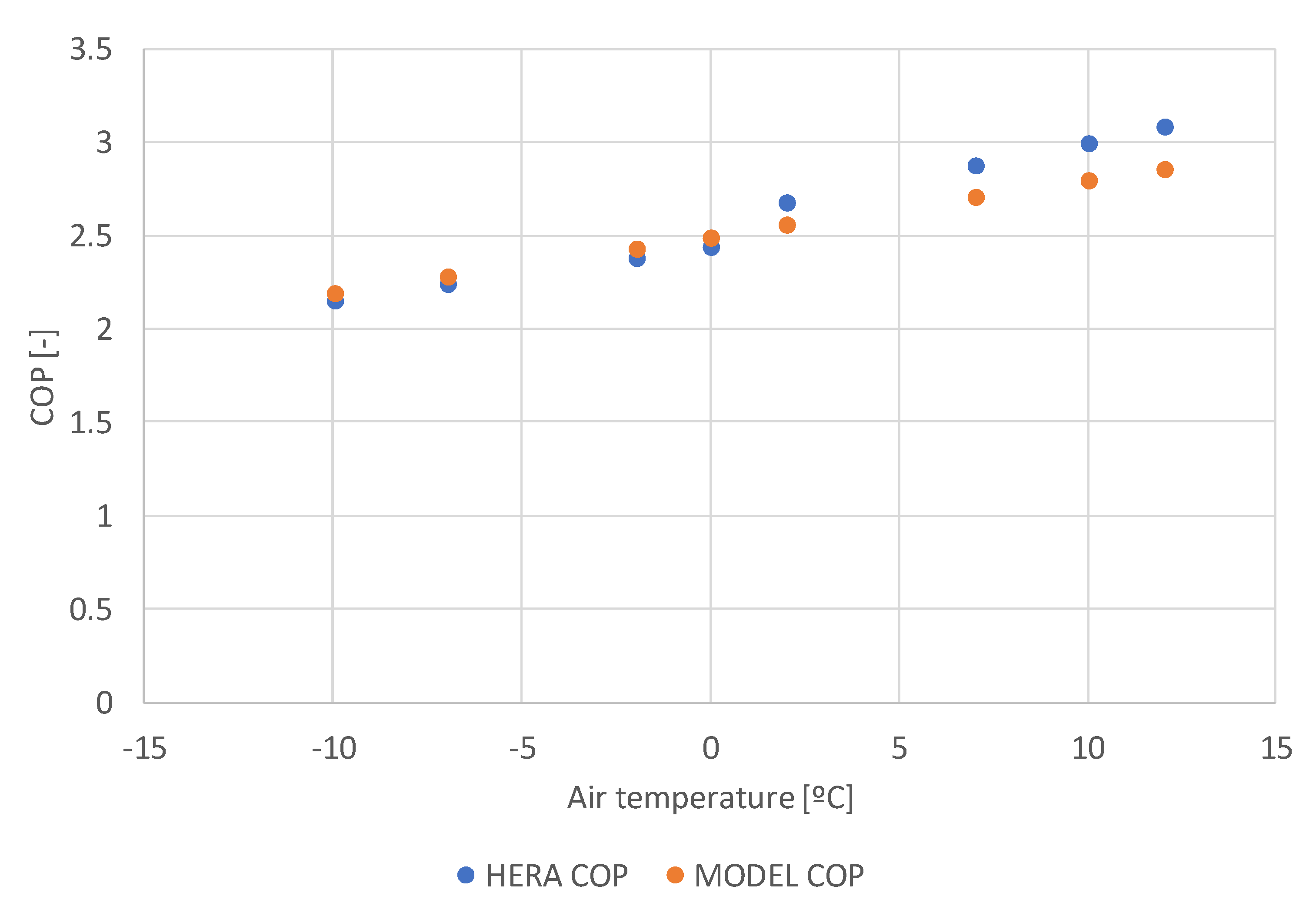However, the use of air source heat pumps is not common in Spain, as it can be followed from the support to these devices in the last release of the Spanish Technical Building Code [12]. In this sense, the developed heat pump model is not sophisticated, although it is accurate enough, as can be derived from the comparison with a commercial machine. Regarding the heating demand forecasting model, a simpler version has been proposed by the authors [40], but, as a novelty, the version that is used in this manuscript is able to retain information regarding thermal insulation of the building. This information made it possible to assess the effect of energy building retrofitting. Therefore, the aim of this paper is to analyse the feasibility of ASHPWH as active measure to fight energy poverty in dwelling blocks. The environmental and economic assessment performed in this paper can eventually provide insightful information to policy makers for implementing clean and efficient measures to tackle energy poverty.

2. Methodology

2.1. Hourly Heating Demand

Building Technical Code (BTC) in Spain establishes a procedure for assessing the energy demand in both winter and summer as a function of the climate severity index (CSI) [41]. In this work, only heating demand is assessed, so focusing on winter energy needs, because energy poverty studies have been mainly focused on this season [42].

The reference specific demand (RD, kWh/m²) in winter is given by Equation (1), where WSI stands for the winter severity index and

Table 1. Coefficients required to obtain the reference specific demand in winter [41].

	α	β
Single-family house	9.29	54.98
Block dwellings	3.51	39.57

provides the coefficients α and β. The winter severity index is defined in Equation (2), where RAD is the average accumulated global radiation over horizontal surface during January, February, and December (Equation (3)), and DD is the average degree-days (at base temperature T_b = 20 °C) for the same months (Equation (4a)) [43].

Table 2. Coefficients required to obtain the winter severity index (WSI) [43].

a	b	c	d	e	f
−8.35 × 10−3	3.72 × 10−3	−8.62 × 10−6	4.88 × 10−5	7.15 × 10−7	−6.81 × 10−2

provides the coefficients for Equation (2). The calculation of RAD requires the global hourly radiation over horizontal surface (r_k), whereas the calculation of DD requires the hourly temperature difference (ΔT_k), as defined by Equation (4b). Hourly values of $T_k$ are available for each climatic zone in the web site of the BTC [44].

$$RD=\alpha +\beta ·WSI$$

(1)

$$WSI=a·RAD+b·DD+c·RAD·DD+d·RA{D}^2+e·D{D}^2+f$$

(2)

$$RAD=\frac{{\sum }_{k=1}^{24\times 90}{r}_k}{3}$$

(3)

$$DD=\frac{{\sum }_{k=1}^{24\times 90}\mathsf{\Delta }{T}_k}{24\times 3}$$

(4a)

$$\mathsf{\Delta }{T}_k=\{\begin{array}{cc}{T}_b-T_k& if{T}_b>T_k\\ 0& otherwise\end{array}$$

(4b)

$RD$ and $WSI$ are overall values, that is, they are calculated for the complete winter season, as it is observed in Equations (1) and (2). Based on these equations, a Taylor series expansion of first order around $\left(RAD,DD\right)$ has been carried out over$WSI$. This procedure leads to an hourly expression of the specific reference demand (Equation (5a)), where: (1) the index “j” is extended from 1 to 4368 (number of hours from January to March and from October to December), (2) $N_d$ is equal to 182 days (number of days in the same period), (3) $N_m$ is equal to 6 (number of months), and (4) the star denotes that this specific reference demand needs to be corrected. This correction has to be done to take into account two different issues. Firstly, the effect of the radiation and second, the fact that three additional months have been included with respect to the original correlation.

The correction of the radiation is performed because, sometimes, its value is high enough to result in a cooling demand (negative heating demand). In this case, the heating demand is set to zero. On the other hand, to consider the inclusion of additional months in the formulation, a reduction coefficient (C_r) is defined as the ratio of the actual specific seasonal demand ($R{D}_{}^a$, given in regulations [45] and equal to 53 kWh/m² for Madrid) to the summation of $R{D}_j^{*}$ over the 4368 h. Accordingly, the corrected hourly specific reference demand $\left(R{D}_j^{}\right)$ is given in Equation (5d).

$$R{D}_j^{*}=\frac{\alpha +\beta ·\left(WSI-\rho ·RAD-\delta ·DD\right)}{24·N_d}+\left(\frac{\beta ·\rho }{N_m}\right)·r_j+\left(\frac{\beta ·\delta }{24·N_m}\right)·\mathsf{\Delta }{T}_j$$

(5a)

$$\rho =a+2·d·RAD+c·DD$$

(5b)

$$\delta =b+c·RAD+2·e·DD$$

(5c)

$$R{D}_j^{}=R{D}_j^{*}·\underset{\underset{C_r}{⏟}}{\underset{}{\left(\frac{R{D}^a}{{\sum }_{j=1}^{4368}R{D}_j^{*}}\right)}}·\{\begin{array}{cc}1& ifR{D}_j^{*}>0\\ 0& otherwise\end{array}$$

(5d)

Once the hourly specific reference demand is obtained, it should be corrected according to the energy performance index (EPI) and the ratio of the reference demand of the whole stock of reference buildings to the 10-th percentile of this stock (R) [41]. This correction leads to the calculation of the hourly absolute demand (D_j, Equation (6)), where the heated area (A) has been included. In Equation (6), the EPI is obtained from the energy performance certificate of the building and R is given at

Table 3. Values for R in Equation (6) [41].

Winter Climatic Zone	Single-Family House	Block Dwellings
A	1.7	1.7
B	1.6	1.7
C	1.5	1.7
D	1.5	1.7
E	1.4	1.7

, where the climatic zone ranges from mild winter (A) to severe winter (E). For the current research, the EPI values have been calculated by cross-correlating the CENSUS 2011 data [46] and the buildings-energy-certification data [47]. The average EPI values for D zone (Madrid) are found to be 3.53 for block dwellings built before 1981, 2.18 if they were built between 1981 and 2007 and 0.92 for the ones built after 2008. Vulnerable households typically live in old buildings and use inefficient heating installations, typically electric radiators, as shown in the literature [48,49,50]. For this reason, the first two building age categories are those in which this collective of households is commonly located. In this study, as explained in Section 3.2, the block dwellings built between 1981 and 2007 are chosen as the baseline case.

$$D_j=A·R{D}_j·\left(\frac{1+\left(EPI-0.6\right)·2·\left(R-1\right)}{R}\right)$$

(6)

Figure 1 displays the hourly demand for each ambient wet bulb temperature (Wet bulb temperature is used as a measurement of the enthalpy of humid air). It shows a cloud of points following a linear regression curve (enclosed in a red dashed line), along with a set of disperse data with lower heating demand. The data density increases with the temperature, in agreement with the radiation issue previously explained.

Finally, the hourly demand is sorted from maximum to minimum, obtaining the annual cumulative heating demand profile, as shown in Figure 2.

2.2. Heat Pump Model

Two models have been developed for obtaining the performance of the heat pump: one for the best efficiency point (BEP) and another for the off-design operation. The former is used to size the main components and the latter to obtain the performance map. The heat pump uses the air as thermal source. Thus, a rotational speed control (inverter) driving the compressor motor is assumed to avoid the loss of heating capacity when the ambient temperature decreases. The nominal rotational speed is taken as 1490 rpm, with a range of variation from 745 to 2235 rpm (±50%). Out of these limits, a back-up system is necessary, assumed as a condensing boiler with modulation, fuelled by natural gas. The efficiency of this boiler has been taken as 95% (based on higher heating value, HHV), assumed constant when considering the usual seasonal performance factor values that were reported by manufacturers [51]. The rotational speed of the evaporator fan is also controlled to keep constant the temperature drop in the air to further improve the heat pump efficiency. The heat pump is an air/water system, so water of the existing radiators heating loop is heated in the condenser. The heat pump takes advantage of the usual oversizing employed in the radiators heat transfer area to make them behave as low temperature radiators, thus enabling the use of heat pump as heater. Domestic hot water demand is covered by solar thermal energy that is supported by natural gas, with this aspect being out of the scope of this analysis. Cooling demand is not considered, according to the common trend in energy poverty studies [42].

Figure 3 shows a scheme of the heat pump. An adiabatic reciprocating compressor is chosen, in accordance with actual commercial trends [52]. The isentropic efficiency (Equation (7)) is used to model the compressor and the polytropic exponent (n) can be obtained, as shown in Equation (8). The volumetric efficiency (η_v, Equation (9)) is used to set the refrigerant mass flow rate$\left(\dot{m}\right)$. In Equations (7)–(9), h stands for enthalpy, s entropy, p pressure, v specific volume, vs. swept volume, r pressure ratio, and α relative clearance volume.

The nominal parameters to solve the best efficiency point are:

• Condenser:

  ○

  Heating capacity $\left({\dot{Q}}_c\right)$: 200 kWth

  ○

  Water conditions: 45 °C at condenser inlet (T_wi) and 55 °C at condenser outlet (T_wo). A counterflow heat exchanger is assumed, feeding the water to an existing low temperature radiator system.

  ○

  Outlet refrigerant conditions: saturated liquid and appropriate approach temperature $\left(\mathsf{\Delta }{T}_c\right)$to achieve 5 °C of pinch point (at saturated vapour state). This approach temperature is 13 °C for R290 (propane), which, as will be explained below, has been chosen as the refrigerant of the heat pump.

• Evaporator:

  ○

  Air conditions: 5 °C as ambient wet bulb temperature (taken as evaporator inlet, T_ai)) and −5 °C as wet bulb temperature at evaporator outlet (T_ao). An ambient pressure of 95 kPa is assumed (Madrid exhibits an elevation over the sea level of 655 m).

  ○

  Outlet working conditions: superheating $\left(\mathsf{\Delta }{T}_v\right)$of 5 °C

  ○

  Inlet working conditions: approach temperature $\left(\mathsf{\Delta }{T}_e\right)$of 10 °C

• Compressor:

  ○

  Speed $\left(N\right)$: 1490 rpm

  ○

  Isentropic efficiency $\left({\eta }_s\right)$: 75% (includes motor and inverter efficiencies)

  ○

  Relative clearance volume $\left(\alpha \right)$: 3%.

$${\eta }_s=\frac{h\left(s_1;p_2\right)-h_1}{h_2-h_1}$$

(7)

$$r=\left(\frac{p_2^{}}{p_1^{}}\right)={\left(\frac{v_1^{}}{v_2^{}}\right)}^n$$

(8)

$${\eta }_v=\frac{\dot{m}}{\left(\frac{V_s}{v_1}\right)·\left(\frac{N}{60}\right)}=1-\alpha ·\left(r^{1/n}-1\right)$$

(9)

The condenser is a refrigerant/water counter-flow heat exchanger. Equation (10) shows the energy balance, where ${\dot{m}}_w$ stands for mass flow rate of water. The approach temperature results in a relationship between both fluids (Equation (11)), where refrigerant outlet temperature is the condensation temperature (refrigerant is saturated liquid at state 3), linked to the condensation pressure (Equation (12)). Enthalpy for water is assessed as enthalpy of saturated liquid at the water temperature. No pressure drop is considered (Equation (13)).

$${\dot{Q}}_C=\dot{m}·\left(h_2-h_3\right)={\dot{m}}_w·\left(h_{wo}-h_{wi}\right)$$

(10)

$$\mathsf{\Delta }{T}_c=T_3-T_{wi}$$

(11)

$$T_3=T_{sat}\left(p_3\right)$$

(12)

$$p_2=p_3$$

(13)

The valve is considered to be adiabatic, so, as kinetic and potential energy are neglected, it is modelled as iso-enthalpic (Equation (14)). Besides, the valve is assumed to be a thermostatic expansion valve, so it keeps the superheating at the compressor suction (Equation (15)) constant by acting on the refrigerant mass flow rate.

$$h_3=h_4$$

(14)

$$\mathsf{\Delta }{T}_v=T_1-T_4=constant$$

(15)

The evaporator is an air/refrigerant cross-flow heat exchanger. Equation (16) gives the energy balance, where ${\dot{m}}_a$ stands for air mass flow rate and $\left({\dot{Q}}_E\right)$ stands for the rate of heat transfer. As in the condenser, the approach temperature establishes a relationship between the fluids (Equation (17)), where refrigerant inlet temperature is the evaporation temperature (refrigerant is a liquid-vapor mixture at state 4), linked to the evaporation pressure (Equation (18)). No pressure drop is considered (Equation (19)).

$${\dot{Q}}_E=\dot{m}·\left(h_1-h_4\right)={\dot{m}}_a·\left(h_{ai}-h_{ao}\right)$$

(16)

$$\mathsf{\Delta }{T}_e=T_{ao}-T_4$$

(17)

$$T_4=T_{sat}\left(p_4\right)$$

(18)

$$p_4=p_1$$

(19)

The main performance parameters of the heat pump in its nominal point (BEP) are the heating capacity (useful heat released in the condenser), previously defined, the compressor consumption ($\dot{W}$, Equation (20)), and the COP (Equation (21)). In the design point, all of them are instantaneous values; later on, in the off-design operation, they will be redefined as seasonal parameters, i.e., both the power rates (${\dot{Q}}_C$ and $\dot{W}$) and the instantaneous COP will be time-integrated.

$$\dot{W}=\dot{m}·\left(h_2-h_1\right)$$

(20)

$$\mathrm{COP}=\frac{{\dot{Q}}_C}{\dot{W}}$$

(21)

The refrigerant must comply with regulations about the global warming potential (GWP) and ozone depletion potential (ODP) [11] of the European Union. Accordingly, R-290 (propane) is chosen as fluid valid for long term, due to the fact that it is a natural refrigerant with null ODP and a GWP value of 3. On the other hand, it is included in the A3 class of the flammability safety classification (ASHRAE), thus considered highly flammable. Figure 4 shows the pressure-enthalpy diagram for R-290, where the assumptions previously stated for the best efficiency point are represented. This diagram shows that the compressor discharge temperature is not too high and the de-superheating interval is small (around 20% of the overall heating capacity). Both of the values are in accordance with the fact that domestic hot water is heated by using other procedures.

The main parameters of the heat pump are fixed once the design point has been solved.

Table 4. Main parameters of the heat pump calculated in the design point and set as constant in off-design operation.

Heat Pump Parameter
Swept volume, vs. (cm3/rev)	4558
Polytropic exponent, n (-)	1.075
Condenser approach, ΔTc (°C)	13
Evaporator approach, ΔTe (°C)	10
Temperature drop at air, $T_{ai}-T_{ao}$(°C)	10
Superheating at compressor suction, ΔTv (°C)	5
Water inlet temperature, Twi (°C)	45
Water outlet temperature, Two (°C)	55

summarises these values. At this point (inlet air temperature of 5 °C and outlet water temperature of 55 °C, usually known as A5/W55), the heating capacity is set as 200 kWth, the compressor consumption is found to be 76.15 kWe, and then the COP results in 2.626.

The modelling of the BEP and the off-design operation have been carried out for different purposes. On one hand, the model of the BEP is developed to define the heat pump parameters that determine its size (listed in Table 4). On the other hand, the off-design model aims to obtain the performance of the heat pump as a function of both the ambient temperature and the heating load, in order to work out the seasonal performance of the device. The input variables are the ambient wet bulb temperature and the rotational speed of the compressor. Equations (8)–(21) are now solved using the parameters that are given in Table 4. It should be noted that the isentropic efficiency of the compressor is replaced by the polytropic relationship (Equation (8)) and the mass flow rates of refrigerant, air, and water are now unknown. Approach temperatures in the heat exchangers have been fixed, while assuming that the number of transfer units are high enough to work in the asymptotic range of effectiveness. The main functions of the off-design model are listed in Equations (22) and (23), which lead to Equation (24). Another limit should be imposed: the maximum driving power of the motor, being assumed as 1.5 times the power consumed at BEP.

$${\dot{Q}}_C={\dot{Q}}_C\left(T_{ai},N\right)$$

(22)

$$\mathrm{COP}=COP\left(T_{ai},N\right)$$

(23)

$$\dot{W}=\frac{{\dot{Q}}_C\left(T_{ai},N\right)}{COP\left(T_{ai},N\right)}=\dot{W}\left(T_{ai},N\right)$$

(24)

2.3. Coupling of the Demand and Heat Pump Models

Once the hourly heating demand (Equation (6)) and the heat pump performance (Equations (22) and (24)) are determined, the map of the device coupled to the demand can be obtained, producing a diagram similar to the one that is shown in Figure 5. In this chart, the heating demand only considers the linear regression curve for the sake of clarity. At the nominal rotational speed, a positive slope line determines the heating capacity of the heat pump for each temperature. This line cuts to the heating load line in one point. To modulate the response of the heat pump, the rotational speed is varied, therefore sweeping the operation zone and cutting to the load curve in a large range. For temperatures out of that range, the back-up system operates (if the load is higher than the heat pump capacity) or the machine is operated in on/off mode, in order to adapt the excess of capacity to the low demand.

Thus, the consumption of the heat pump (${\dot{W}}_j)$and the back-up system (${\dot{F}}_j^{bkp})$ (if any) to meet the demand are calculated, for each operation hour, while using the functions that are given in Equation (25a–d). In Equation (25c), bkp stands for the back-up system, assumed as a natural gas condensing boiler with a constant efficiency (${\eta }_{bkp}$) value of 95% on higher heating value basis. In the same equation, $\dot{F}$ stands for the natural gas consumption (again based on HHV) of the back-up system. Equation (25d) determines the power of the back-up boiler (${\dot{Q}}_{bkp}$). In the on/off operation range, the demand is covered by the heat pump working at the minimum rotational speed, as it is derived from the algorithm described in Equation (25). Defrosting cycles are neglected, due to the usually low air moisture content in Madrid [53].

$${\dot{Q}}_{C,j}^{max}=max\left\{{\dot{Q}}_C\left(T_{ai,j},N_{max}\right),COP\left(T_{ai,j},N_{max}\right)·1.5·\dot{W}\left(T_{ai,j}^{design},N_{design}\right)\right\}$$

(25a)

$${\dot{W}}_j=\{\begin{array}{cc}{\dot{Q}}_{c,j}/COP\left(T_{ai,j},N_j\right)& if{D}_j^{}\le {\dot{Q}}_{C,j}^{max}\\ {\dot{Q}}_{C,j}^{max}/COP\left(T_{ai,j},N_j\right)& otherwise\end{array}$$

(25b)

$${\dot{F}}_j^{bkp}=\{\begin{array}{cc}0& if{D}_j^{}\le {\dot{Q}}_{C,j}^{max}\\ \left(D_j^{}-{\dot{Q}}_{C,j}^{max}\right)/{\eta }_{bkp}& otherwise\end{array}$$

(25c)

$${\dot{Q}}_{bkp}=max\left\{{\dot{F}}_j^{bkp}\right\}$$

(25d)

Some seasonal performance indexes have been defined: heating seasonal performance factor (HSPF, Equation (26)), CO₂ avoided ratio (AVCO2, Equation (27)) and renewable input to heating demand ratio (R2H, Equation (28)). Numerical coefficients that are employed in Equations (27) and (28a) make it possible to consider the environmental impact of the electricity coming from the grid to drive the heat pump. They have been taken from [54], according to the Spanish energy sector. Equation (28b) comes from the current EU regulation regarding the support to heat pumps [10].

$$HSPF=\frac{{\sum }_{j=1}^{4368}{\dot{W}}_j·COP\left(T_{ai,j},N_j\right)}{{\sum }_{j=1}^{4368}{\dot{W}}_j}$$

(26)

$$AVCO2=\frac{\left(\frac{{\sum }_{j=1}^{4368}{D}_j}{{\eta }_{bkp}}\right)·0.252-\left[0.331·{\sum }_{j=1}^{4368}{\dot{W}}_j+0.252·{\sum }_{j=1}^{4368}{\dot{F}}_j^{bkp}\right]}{{\sum }_{j=1}^{4368}{D}_j}$$

(27)

$$R2H=\frac{{\sum }_{j=1}^{4368}RE{S}_j+0.414·{\sum }_{j=1}^{4368}{\dot{W}}_j}{{\sum }_{j=1}^{4368}{D}_j}$$

(28a)

$$RE{S}_j=\{\begin{array}{c}{\dot{Q}}_{C,j}^{}·\left(1-\frac{1}{HSPF}\right)ifHSPF\ge 2.5275\\ 0otherwise\end{array}$$

(28b)

2.4. Economic Model

The main indicator to assess the economic feasibility of this kind of device is the levelised cost of heating (LCOH), which integrates both the investment and operating costs [55]. In this research, two LCOH have been calculated: one referred to the whole heating demand ($LCO{H}_{DB}\left[€/MWh\right]$, (Equation (29a)) and another referred to the whole heated area ($LCO{H}_{AB}\left[€/m^2\right]$ (Equation (29b)). In Equation (29a), INV stands for investment, C for annual cost, superscript M refers to maintenance, W to power consumption, F to fuel consumption, subscript 0 to costs in year zero, CRF to the capital recovery factor (Equation (29c)), CELF stands for the constant escalation levelisation factor (Equation (29d)). In Equations (29c–e), r_x represents the nominal escalation rate of the item x, wacc the weighted average capital cost, and Ny is the life span of the project.

$$LCO{H}_{DB}=\frac{\left(IN{V}_{HP}+IN{V}_{bkp}\right)·CRF+C_0^W·CEL{F}^W+C_0^F·CEL{F}^F+C_0^M·CEL{F}^M}{{\sum }_{j=1}^{4368}{D}_j}$$

(29a)

$$LCO{H}_{AB}=LCO{H}_{DB}·\left[\frac{{\sum }_{j=1}^{4368}{D}_j}{A}\right]$$

(29b)

$$CRF=\frac{wacc·{\left(1+wacc\right)}^{Ny}}{{\left(1+wacc\right)}^{Ny}-1}$$

(29c)

$$CEL{F}_x=\left[\frac{k_x·\left(1-k_x^{Ny}\right)}{1-k_x}\right]·CRF$$

(29d)

$$k_x=\frac{1+r_x}{1+wacc}$$

(29e)

The investment for the heat pump (inverter model with 200 kWth of heating capacity) has been taken as 24,753 € [52], and a scale law has been fit for the investment of the back-up boiler (Equation (30)).

$$IN{V}_{bkp}[€]=1087.6·{\dot{Q}}_{bkp}^{0.506}\left[k{W}_{th}\right]$$

(30)

For consumptions with installed power higher than 15 kWe, the cost of electricity includes a term for maximum consumed power in a year and a term for annual consumed energy. Moreover, this consumption considers hourly discrimination in three periods (P1, P2, and P3), according to

Table 5. Electrical tariff [56].

Period	Power Term (€/kW) 1	Energy Term (€/MWh)
P3: 0.00 to 8.00	16.7803	85.3
P2: 8.00 to 18.00	25.1704	114.1
P1: 18.00 to 22.00	41.9507	127.1
P2: 22.00 to 24.00	25.1704	114.1

¹ The cost associated to the power term is derived from multiplying the tariff by the maximum power consumed along the year at each period.

.

For comparison purposes, two additional scenarios have been considered: a decentralised system and a centralised one, both using only condensing natural gas boilers with the same efficiency as the back-up boiler (95% based on HHV). In the de-centralised boiler case, 60 single dwellings of 100 m² are considered, each employing a natural gas boiler with an investment of 800 € and maintenance costs of 150 €/year. In the centralised boiler scenario, a larger boiler is used to meet the overall demand, being given its investment by Equation (30) and a maintenance cost assumed of 2000 €/year.

All of the costs include taxes. Regarding the natural gas costs, two tariffs have been selected, depending on the annual consumption. Accordingly, for large consumptions (centralised cases in both heat pump with back-up and boiler alone) the tariff is 971.64 €/year plus 40.66 €/MWh (based on HHV), whereas for small consumptions (decentralised boilers) the tariff is 115.98 €/year plus 42.4 €/MWh (again based on HHV) [57].

Maintenance cost has been set to 2000 €/year for the proposed system (heat pump supported by a boiler).

Table 6. Assumed economic parameters.

Parameter	Value
Weighted average capital cost, wacc (%)	0
Nominal rate of power, rW (%)	5
Nominal rate of gas, rF (%)	5
Nominal rate of maintenance, rM (%)	2.5
Life span, Ny (years)	15

shows the economic parameters used to calculate the levelised costs.

3. Results

3.1. Heat Pump Model

Once the model is completed, Equations (22)–(24) are solved, obtaining, respectively, Equations (31)–(33). For a given rotational speed, the relation between heat capacity and air temperature is linear, and the slope increases with the speed, as it can be seen in Equation (31). Regarding the COP, Equation (32) is obtained, but it does not depend on rotational speed. This result is foreseeable, because the COP is the ratio between heat capacity and compressor consumption, both proportional to the mass flow rate, which is directly dependent on the rotational speed. Combining both Equations (31) and (32), the expression for the compressor consumption is obtained (Equation (33)).

$${\dot{Q}}_C=\left(0.1106·N+0.0002\right)+\left(0.0053·N+0.0003\right)·T_{ai}$$

(31)

$$\mathrm{COP}=2.49499+0.02981·T_{ai}$$

(32)

$$\dot{W}=\frac{\left(0.1106·N+0.0002\right)+\left(0.0053·N+0.0003\right)·T_{ai}}{2.49499+0.02981·T_{ai}}$$

(33)

Figure 6 shows the iso-lines of heating capacity as a function of the rotational speed and the ambient wet bulb temperature. The limitation of maximum electrical power (Equation (25a)) has been taken into account.

A comparison with an actual machine has been performed in order to validate the results of the heat pump model. A literature search has been carried out to find an existing device that fits with the characteristics of the modelled one. The selected equipment has been HERA 190-2-2 [58], an air to water heat pump from EUROKLIMAT. A reciprocating compressor using an inverter drives it and it has a design heating capacity of 190 kWth. The refrigerant is R290 as the one selected in this paper. The water outlet temperature of the existing heat pump is 55 °C, as in the model. Figure 7 plots the comparison of the COP, showing a good match, especially at low temperatures. This behavior is due to the fact that the HERA 190-2-2 data are based on dry bulb air temperature, whereas the data from the model are based on the wet bulb temperature, with both temperatures being very similar at low dry bulb temperature.

3.2. Baseline Case

A block dwelling with an overall heated area of 6000 m² and EPI of 2.18, i.e., built between 1981 and 2007, located in Madrid, has been simulated. It is important to point out that the selected baseline-building-age represents a considerable percentage of vulnerable households in Spain and the 41% of the overall main houses with heating [46]. Figure 2 shows its annual cumulative heating demand profile. Applying the algorithm given by Equation (25) to each winter hour, the results that are shown in

Table 7. Energy results in the baseline case.

Parameter	Value
Seasonal heating demand, $\sum _{j=1}^{4368}{D}_j$ (MWh)	600.833
Heating demand met by heat pump, $\sum _{j=1}^{4368}{\dot{W}}_j·CO{P}_j$ (MWh)	576.675
Seasonal consumption of heat pump, $\sum _{j=1}^{4368}{\dot{W}}_j$ (MWh)	223.080
Back-up boiler consumption, $\sum _{j=1}^{4368}{\dot{F}}_j^{bkp}$ (MWh)	25.430
Size of back-up boiler, ${\dot{Q}}_{bkp}$ (kW)	180
Renewable energy taken from the ambient air, $\sum _{j=1}^{4368}RE{S}_j$ (MWh)	445.949

are obtained. From these values, the performance indexes that are given by Equations (26)–(28) are calculated, and

Table 8. Performance indexes in the baseline case.

Parameter	Value
Heating seasonal performance factor, HSPF (-)	2.585
Avoided CO2 emissions, AVCO2 (g CO2/kWht)	131.7
Renewable to heating demand ratio, R2H (%)	74.22

summarises the results. Furthermore, Figure 8 shows the contribution to the heating demand of both the heat pump (96%) and the back-up boiler (4%).

At low thermal demands, the heat pump is controlled in on/off mode due to the minimum rotational speed limit. This type of control causes important energy losses when an inverter is not available, but this driving control is expected to reduce them. Accordingly, Figure 9 shows the cloud of points for the thermal demand under the minimum heat capacity line. Once these points are sorted and moved into the ASHPWH contribution to the annual cumulative heating demand profile, they take up the end tale of the distribution (Figure 10), accounting for 8% of the overall demand that is met by the heat pump. Figure 9 also shows that the motor consumption ranges between 31.2 to 49.9 kWe (41 to 65.5% as compared to the consumption at design point). This allows for us to assume that low current peaks will take place in the startups and, moreover, they also will be smoothed by the use of the speed modulation. On the other hand, the ratio of the thermal demand to the minimum heating capacity of the heat pump at each hour determines the time fraction when the heat pump has been working over that hour. Figure 11 shows this ratio, after being sorted. It can be observed that in 58% of the time when the heat pump was working in on/off mode was “on” more than 30 min (hour fraction 0.5), therefore minimizing the transitory effect on the components of the heat pump. In summary, the availability of the inverter is expected to significantly contribute to reducing the energy losses of the on/off operation mode and, consequently, it make sense to neglect it for the scope of the current analysis.

Regarding the costs,

Table 9. Levelised costs in the baseline case for heat pump, de-centralised, and centralised boilers.

Levelised Costs	Heat Pump	De-Centralised Boiler	Centralised Boiler
Levelised cost of heating (demand based), LCOHDB (€/MWh)	92.22	108.55	73.54
Levelised cost of heating (area based), LCOHAB (€/m2)	9.23	10.87	7.36

summarises the results.

Figure 12 shows the breakdown of the levelised costs that are given in Table 9. As the demand and the heated area are established, the percentage breakdown is the same for both levelised costs (see Equation (29a,b)). Moreover, Figure 12 points out the predominance of operating costs (especially the energy term, being the maintenance less significant) over investment (heat pump and boiler).

The proposed active measure should be supplemented by the application of a social tariff based on the cost breakdown. This would make it possible to take advantage of the environmental benefits of the proposed system at the same levelised cost of the most economical system, i.e., the centralised boiler. In this case, a discount of 23.75% in the electricity cost (overall cost, including power and energy terms) would reduce the LCOH to 73.54 €/MWh, matching the cost of the centralised boiler. This discount is in accordance with the current social electricity tariff in Spain [59], which ranges from 25% for vulnerable consumers, 40% for severely vulnerable consumers, and up to 100% for consumers at risk of social exclusion. The average discount was 32% when considering the distribution of each cluster in 2019 (respectively, 648,826 and 630,086 households in the first two categories, and 4545 in the third one [60]). Therefore, the required discount to spread the proposed system would be even lower than the one currently applied to vulnerable-households’ electricity bill.

3.3. Influence of Energy Retrofitting

The baseline case has been selected to be representative of the middle-energy efficiency level pool of dwellings, with an energy performance assessment of E, close to D (EPI = 2.18). However, in the context of energy poverty, it is usual to find dwellings built before 1980 with worse insulation condition than this middle energy-efficiency-level. In these cases, an energy retrofitting of the dwelling is recommended, which makes it possible to reduce the heating cost per dwelling. To assess this fact, Figure 13 has been obtained, varying EPI and maintaining the levelised cost of heating in demand base with the same value as the baseline case. This condition requires varying the heated area, obtaining a potential fitting curve (Equation (34)). In Figure 13 the average EPI obtained for dwelling blocks in Spain have been represented over such fitting curve, so obtaining their heated area to maintain the same levelised cost than in the baseline case.

$$A=11,139·EP{I}^{-0.789}$$

(34)

4. Discussion

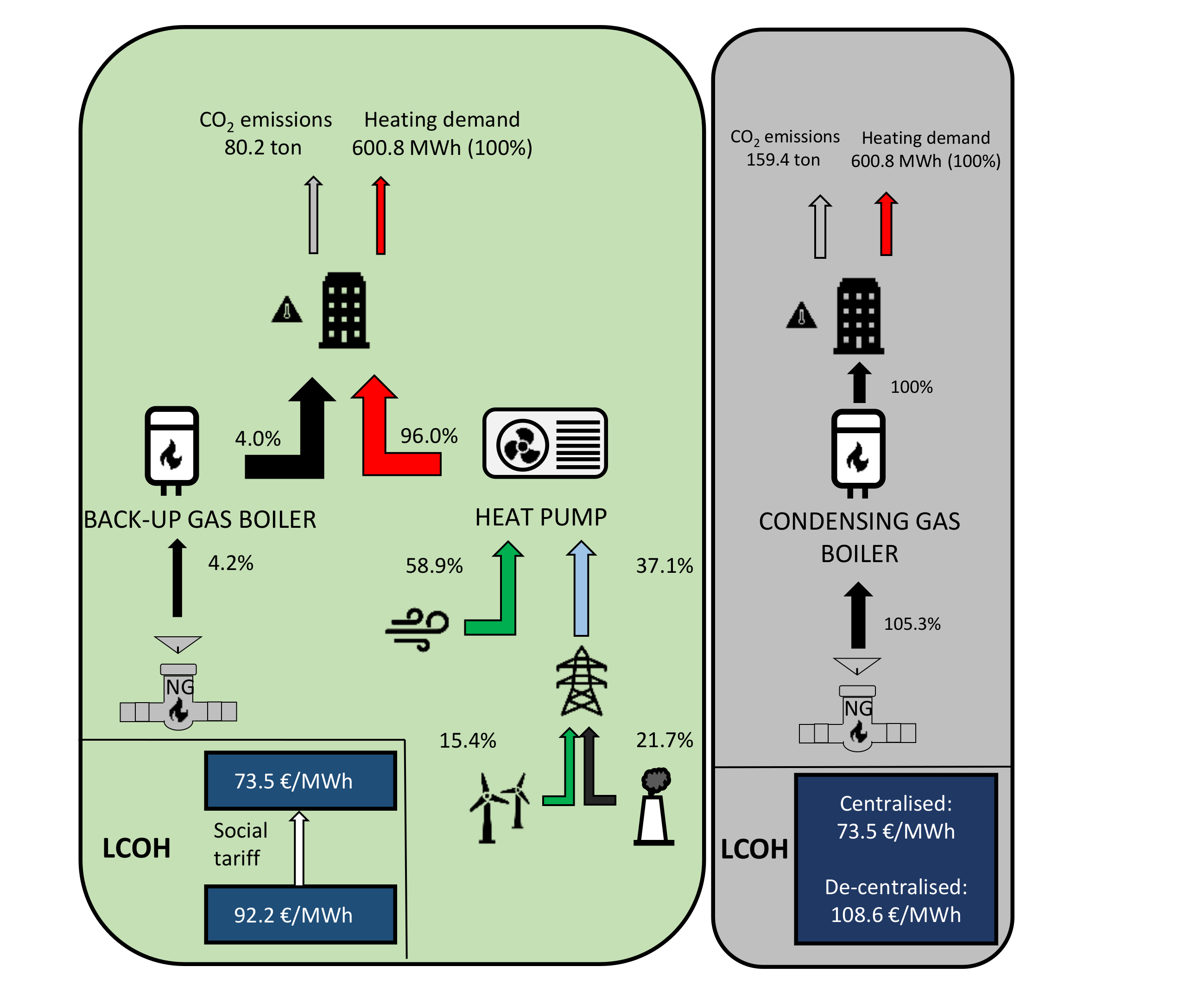
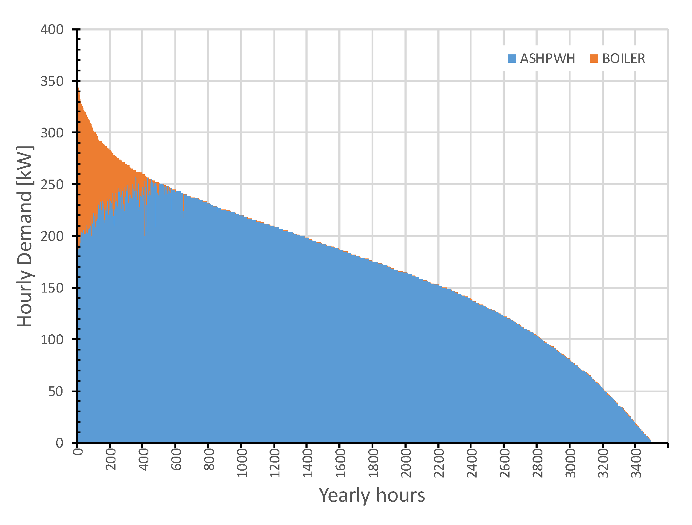
The proposed demand model makes it possible to obtain the hourly demand profile of a building, which is essential for working out the instantaneous consumptions of the heating system. The shape of the annual cumulative heating demand curve is consistent with the profiles that were obtained by other simulation tools [40]. This model only requires the location of the building, its useful area and the energy performance certification (EPC). A detailed simulation of the building thermal behaviour is necessary to assess the EPC, which leads to the EPI that is integrated in the proposed model. The fact that no specific additional information about the building is required by the model makes it very easy-to-use and helpful for planning purposes. The flexibility of the model has been used in order to solve a case study representative of vulnerable dwellings.

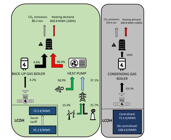
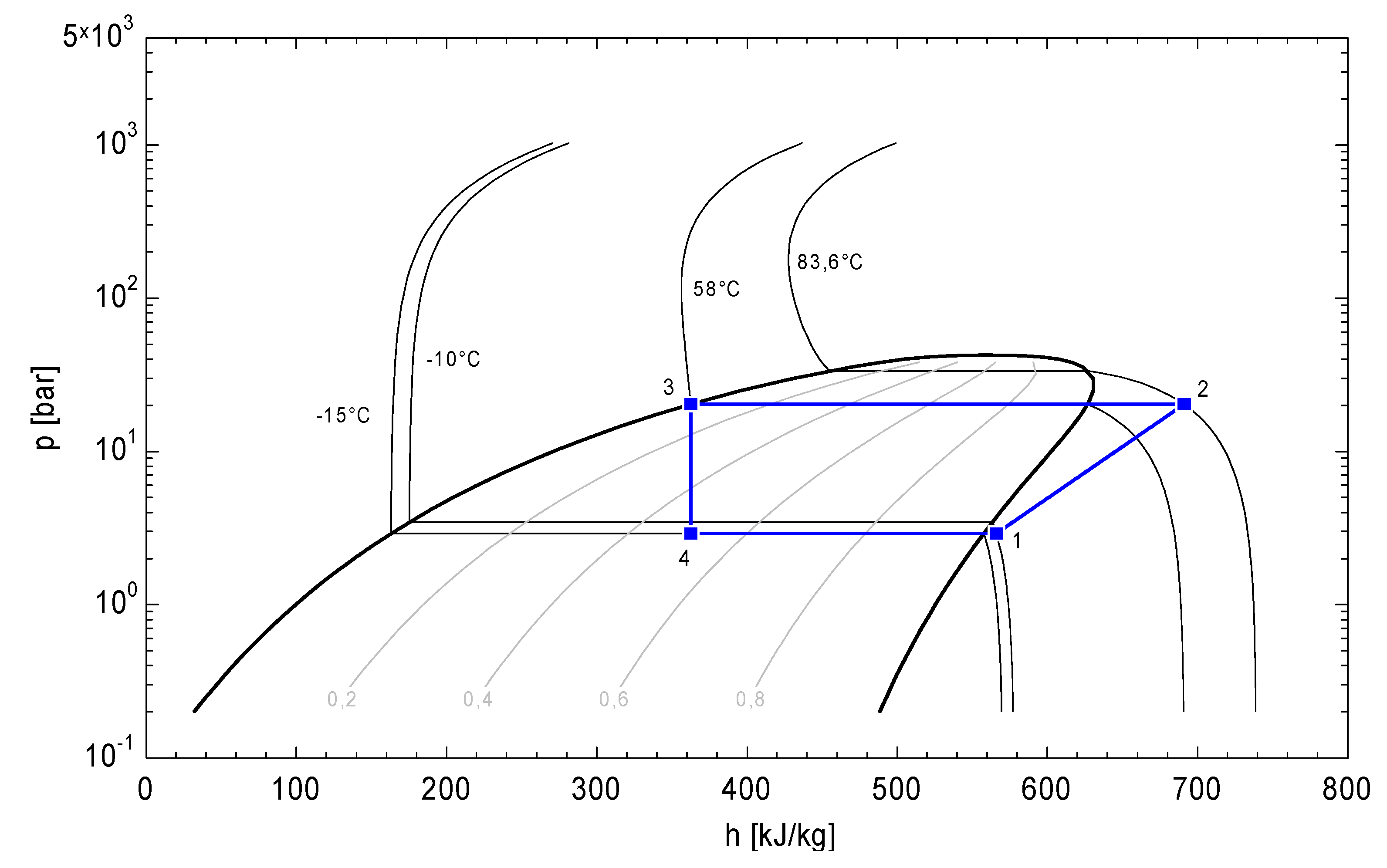
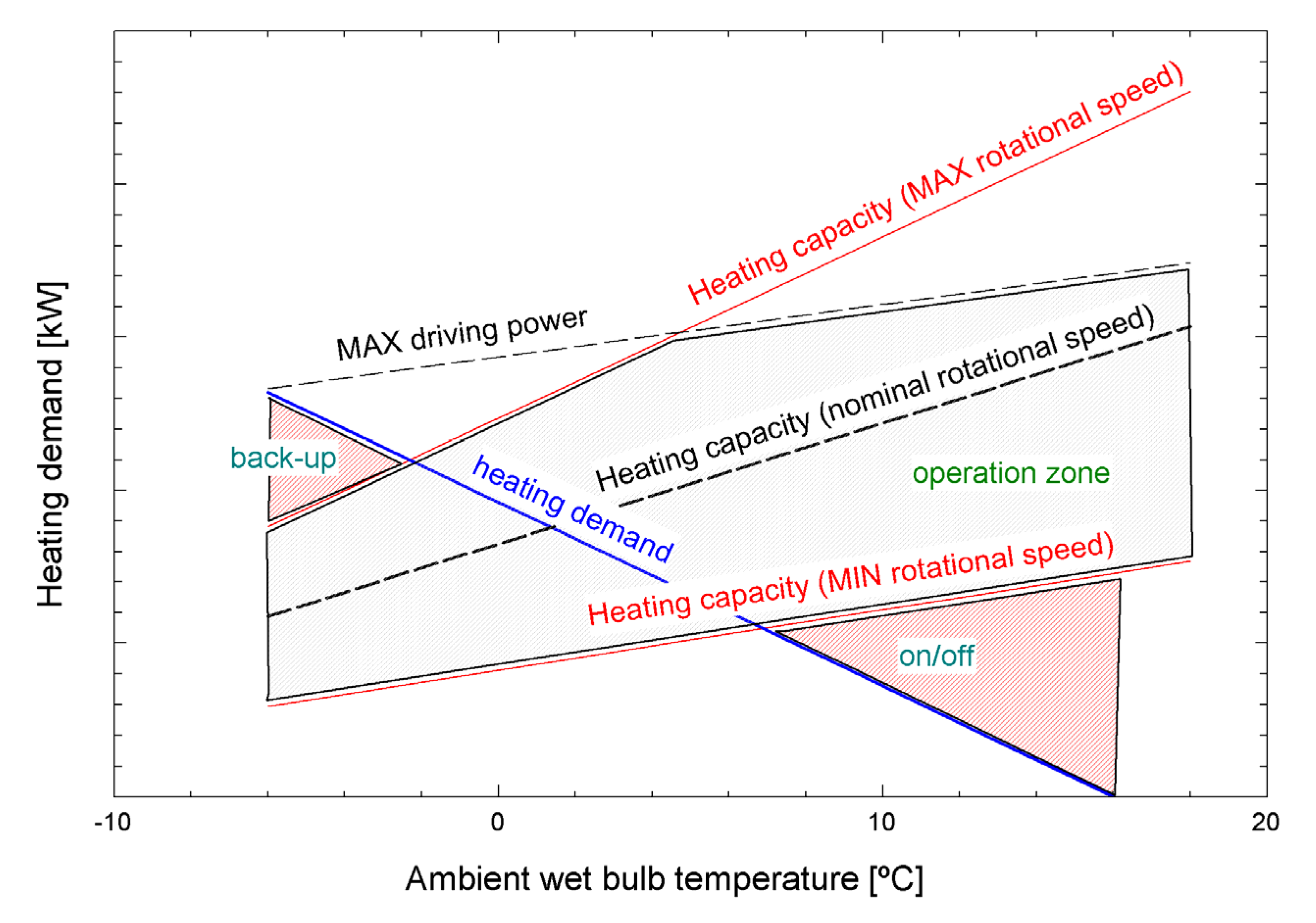
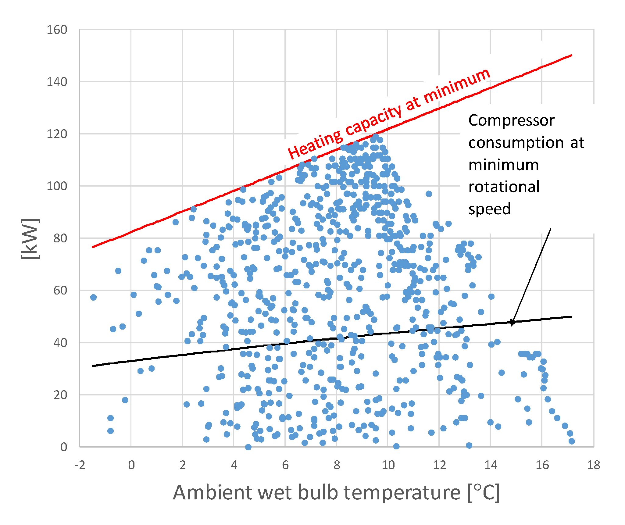
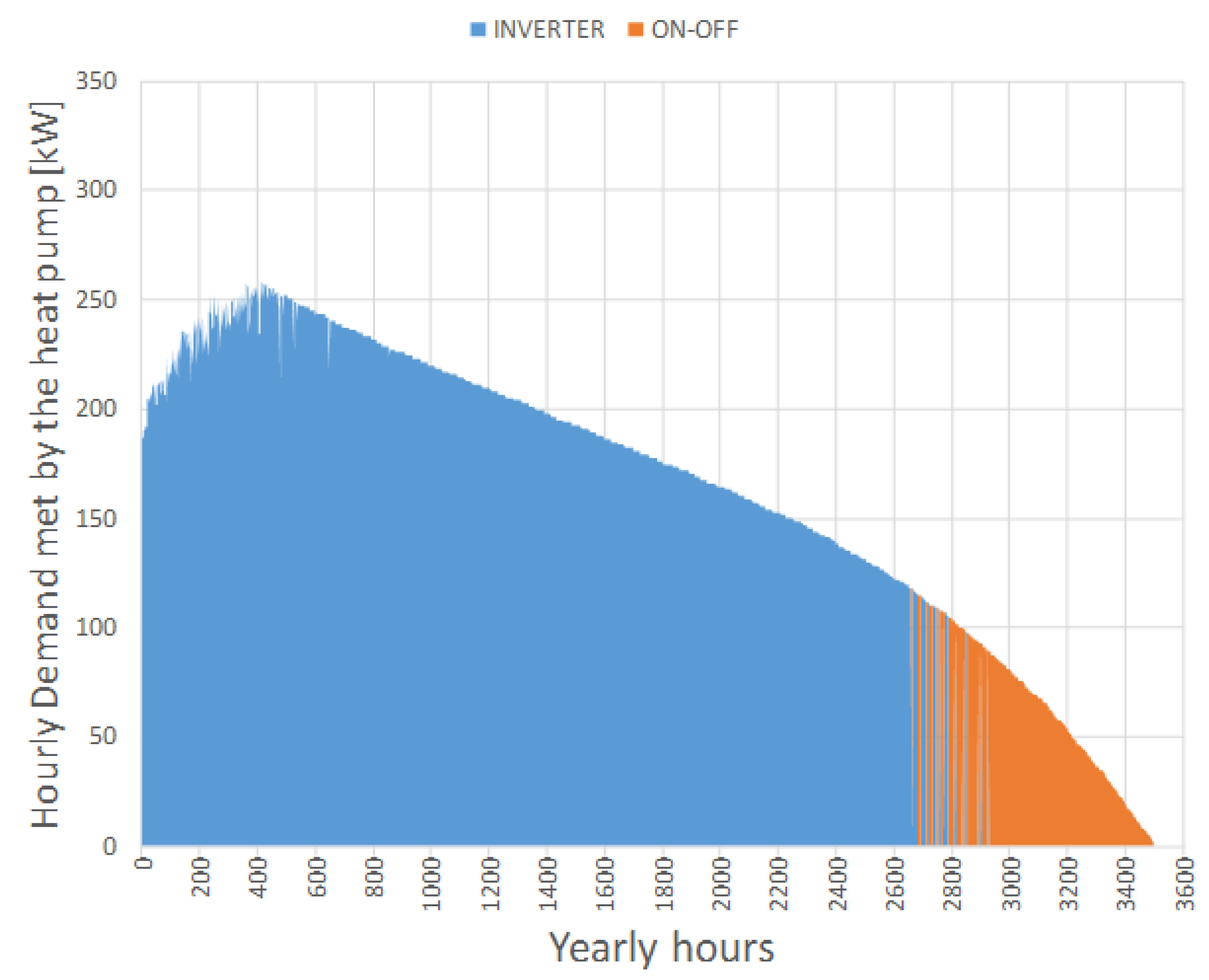
Regarding the heat pump, R290 (propane) has revealed as a suitable refrigerant for this application, and it is also supported by many manufacturers. It is a natural fluid, with zero ODP and very low GWP. The low compressor discharge temperature and the low de-superheating zone in the condenser advise taking this fluid into consideration for the future. Its high flammability is not relevant in the current case, since it is a centralised unit, with roof-top allocation and maintenance performed by professional workers. The speed control in the compressor gives to the heat pump the capability to meet nearly all of the heating demand (96% in the baseline case) with good efficiency. In the baseline case, the heating seasonal performance factor achieved is 2.585, exceeding the minimum that is required to consider the thermal energy taken from the air as renewable energy. Furthermore, the overall renewable energy to meet the heating demand is obtained, taking both the energy supplied by the air and the renewable share in the electricity mix into account (applied to the electricity consumption of the heat pump). Therefore, each kWh-th met with the proposed system avoids the emission of 131.7 g CO₂, whereas 265.3 g CO₂ are emitted if a boiler is used.

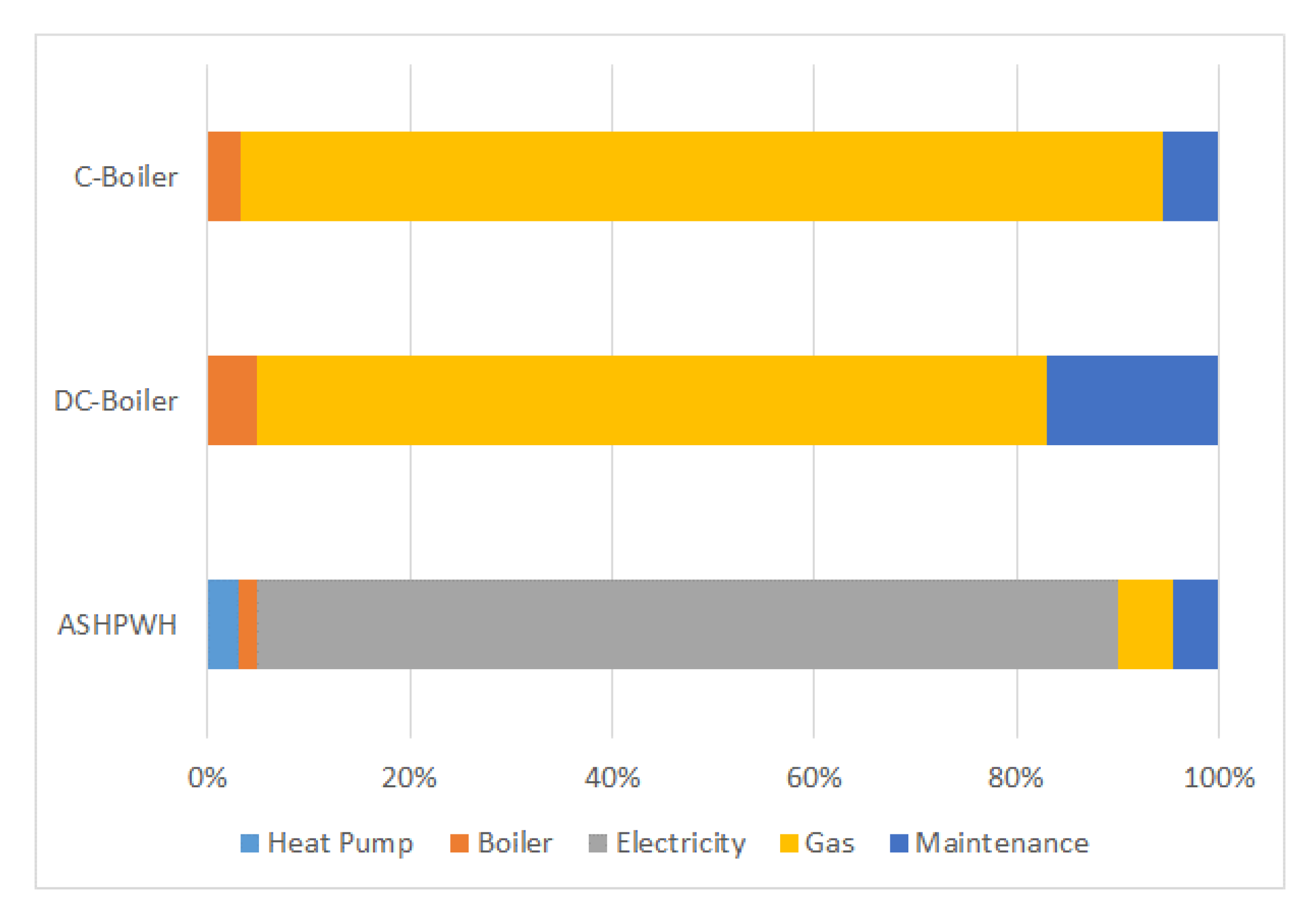
Regarding the cost for the baseline case, the proposed technology (heat pump plus boiler back-up) reduces the levelised cost of heating by 15% with respect to the de-centralised boiler. However, the proposed system increases the cost by 25% with respect to the centralised boiler. On the other hand, with centralised gas neither renewables sources are employed nor carbon dioxide emissions are avoided. The cost breakdown reveals that the energy cost, which facilitates the integration of subsidy policies to the operation, is the most important contribution to the overall cost. Therefore, a discount of 23.75% in electricity bill (comparable with the current social-tariff average-discount) would be enough to equalise the levelised cost of heating of the proposed system with the centralised boiler (the most economical scenario). Furthermore, the innovative and social aspect of this system makes it possible to integrate funding by non-profit organisations, energy companies, Public Administration, or even the actual consumers (depending on their vulnerability level). These subsidies to the proposed system would be endorsed due to its excellent environmental performance, balancing this way de-carbonisation with energy affordability.

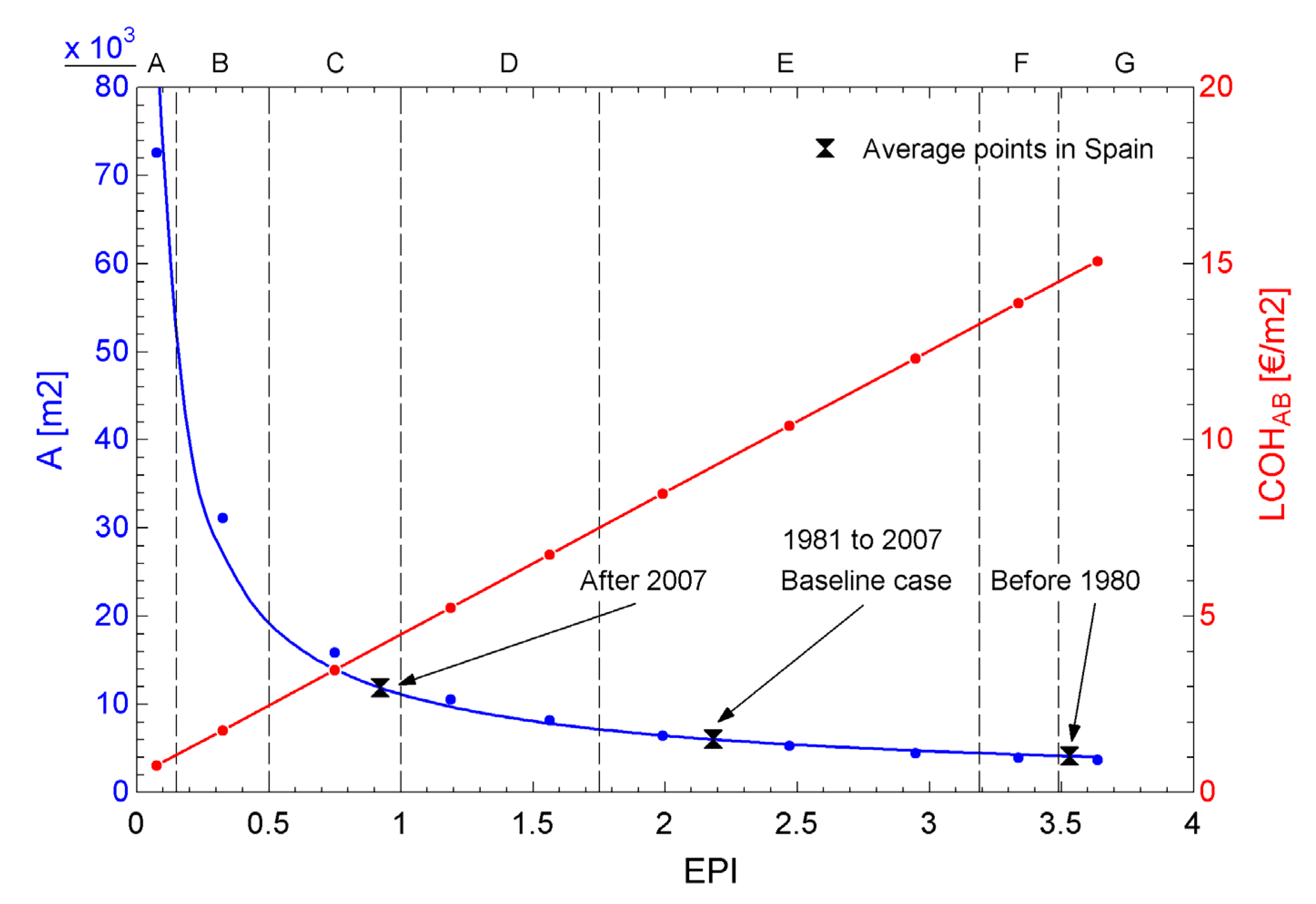
Finally, the effect of energy retrofitting has been investigated. The results show that, if the energy performance assessment is improved from E to C due to a retrofit, the same heat pump would be able to meet the demand of 160 dwellings of 100 m² instead of 60 of the baseline case. Regarding the heating cost per square meter, the cost drops 4 €/m² for every EPI unit reduction. Accordingly, in the same example, the levelised cost of heating decreases 500 € for a dwelling of 100 m² (with a baseline cost of 848 €).

5. Conclusions

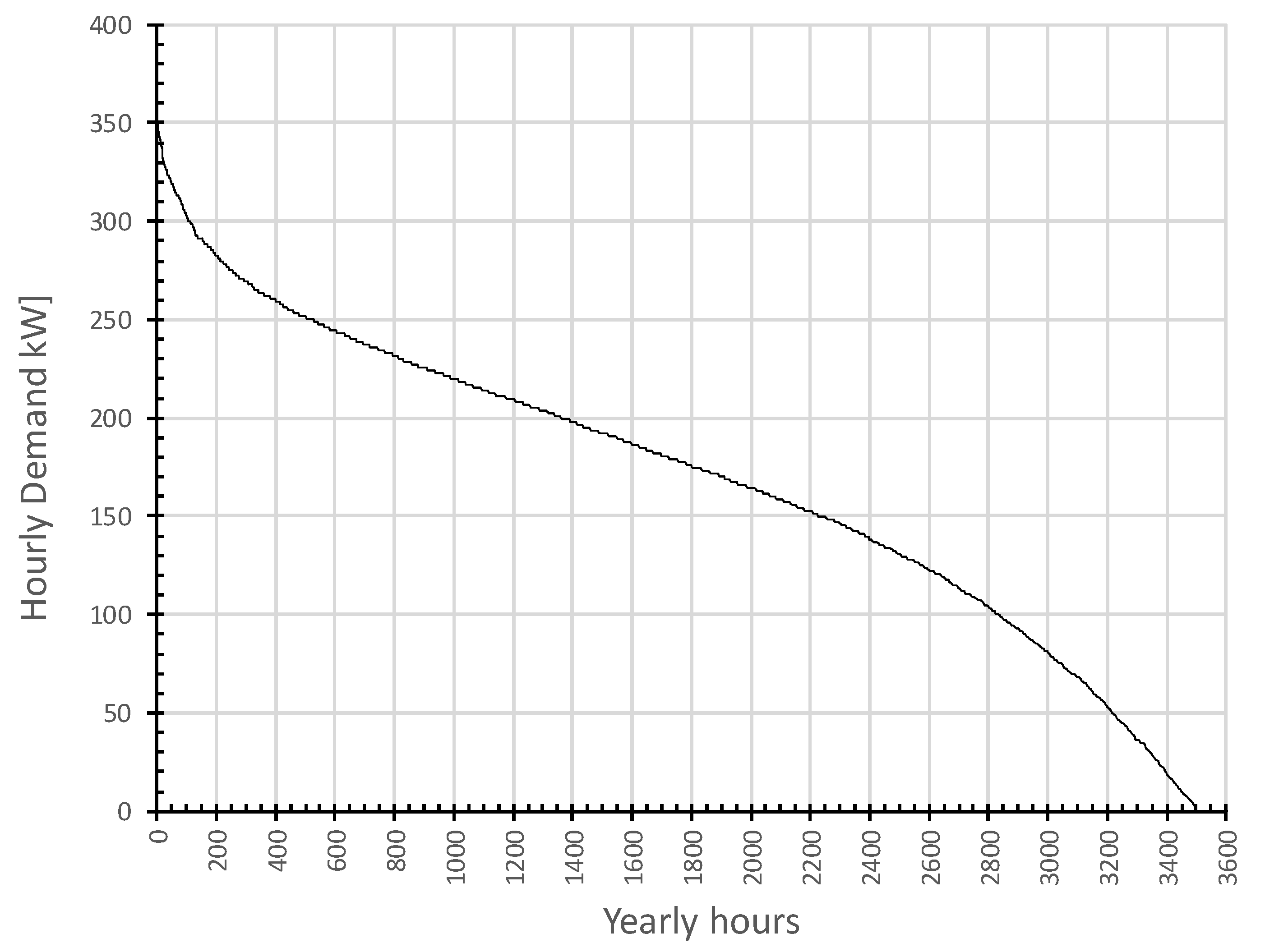
The feasibility of heating a block dwelling in Madrid by an air-source heat-pump water heater has been investigated in the framework of energy poverty research. The implementation of the heat pump is planned as a retrofit of the heating system. Therefore, an existing system that is based on radiators is assumed, and the operation temperatures of the heat pump are adapted to this configuration. A global methodology has been used to forecast the hourly heating demand while using an expansion method that is based on the Spanish regulation. The performance map has been obtained after selecting an eco-friendly refrigerant (R290), and considering a speed variation control over the compressor. This control makes it possible to meet nearly the whole demand with a high efficiency. Finally, the demand has been coupled to the performance of the heat pump.

When considering environmental and efficiency indicators, the obtained results show an excellent behaviour of the heat-pump as compared with the classical solution of the natural gas centralised boiler system. However, the levelised cost of heating is 25% higher than the centralised boiler, due to the low prices of gas for high consumption volumes. In this sense, a discount in electricity bill for vulnerable households might be taken into account, considering both social and environmental benefits, to equalise the energy costs of this technology with the one of a centralised gas boiler. The situation is reversed in the case of comparing the heat pump with the de-centralised boiler solution, with the heating cost of the heat pump being 15% lower than the boiler one. In all the scenarios, the main contribution to the overall cost is the operation, especially the energy cost.

Therefore, the heat pump has revealed as an efficient and sustainable system to tackle energy poverty in a typical case of vulnerable households, such as the building blocks analysed, especially when compared with a de-centralised boiler heating system. In any case, a new electricity tariff frame that reduces the operation costs of heat pumps with respect to the centralised boiler solution would be highly recommended.

In future works, the model will be expanded to summer season (cooling demand), taking advantage of the reversible ability of heat pumps. In the context of energy poverty, this is a new trend, especially in countries in Southern Europe. Other technologies, such as thermally driven heat pumps (both absorption and internal combustion engine), might be also considered to be alternatives. Moreover, the application to the different climatic zones of Spain will be carried out and policy implications will be pointed out.

References

1. Thomson, H.; Bouzarovski, S. Addressing Energy Poverty in the European Union: State of Play and Action. EU Energy Poverty Observatory, European Commission. 2018. Available online: https://www.energypoverty.eu/sites/default/files/downloads/publications/19-05/paneureport2018_updated2019.pdf (accessed on 9 April 2020).
2. EU Statistics on Income and Living Conditions 2017. Available online: https://ec.europa.eu/eurostat/web/microdata/european-union-statistics-on-income-and-living-conditions (accessed on 9 April 2020).
3. Romero, J.C.; Linares, P.; López, X. The policy implications of energy poverty indicators. Energy Policy 2018, 115, 98–108. [Google Scholar] [CrossRef]
4. Ministry for Industry and Ecological Transition, Spanish Strategy to Tackle Energy Poverty. 2019. Available online: https://www.miteco.gob.es/es/ministerio/planes-estrategias/estrategia-pobreza-energetica/actualizaciondeindicadorespobrezaenergetica2019_tcm30-502983.pdf (accessed on 15 April 2020).
5. Dobbins, A.; Fuso Nerini, F.; Deane, P.; Pye, S. Strengthening the EU response to energy poverty. Nat. Energy 2019, 4, 2–5. [Google Scholar] [CrossRef]
6. Boardman, B. Fuel poverty synthesis: Lessons learnt, actions needed. Energy Policy 2012, 49, 143–148. [Google Scholar]
7. Marmot Review Team. The Health Impacts of Cold Homes and Fuel Poverty; The Baring Foundation: London, UK, 2011. [Google Scholar]
8. Cruz Roja Española. La Vulnerabilidad asociada al ámbito de la vivienda y pobreza energética en la población atendida por Cruz Roja. Available online: https://www.cruzroja.es/principal/documents/1789243/2038966/Informe_Cruz_Roja_Boletin_sobre_la_vulnerabilidad_social_N17_Vivienda_Pobreza_Energ%C3%A9tica.pdf/59045195-3960-d9a5-d632-7a92664df97a (accessed on 26 May 2020).
9. Vedavarz, A.; Kumar, S.; Hussain, M.I. HVAC: Handbook of Heating, Ventilation and Air Conditioning for Design and Implementation; Industrial Press Inc.: New York, NY, USA, 2007. [Google Scholar]
10. EUR-Lex. Directive 2009/28/EC of the European Parliament and the Council of 23 April 2009 on the Promotion of the Use of Energy from Renewable Sources and Amending and Subsequently Repealing Directives 2001/77/EC and 2003/30/EC. 2009. Available online: https://eur-lex.europa.eu/legal-content/EN/ALL/?uri=CELEX%3A32009L0028 (accessed on 26 May 2020).
11. EUR-Lex. Regulation (EU) No 517/2014 of the European Parliament and the Council of 16 April 2014 on Fluorinated Greenhouse Gases and Repealing Regulation (EC) No 842/2006. 2014. Available online: https://eur-lex.europa.eu/eli/reg/2014/517/oj (accessed on 26 May 2020).
12. Building Technical Code (Release 2019). Available online: https://www.codigotecnico.org/images/stories/pdf/ahorroEnergia/DBHE.pdf (accessed on 9 April 2020).
13. Underwood, C.P.; Royapoor, M.; Sturm, B. Parametric modelling of domestic air-source heat pumps. Energy Build. 2017, 139, 578–589. [Google Scholar] [CrossRef] [Green Version]
14. Lohani, S.P.; Schmidt, D. Comparison of energy and exergy analysis of fossil plant, ground and air source heat pump building heating system. Renew. Energy 2010, 35, 1275–1282. [Google Scholar] [CrossRef]
15. Tangwe, S.; Simon, M.; Meyer, E.L.; Mwampheli, S.; Makaka, G. Performance optimization of an air source heat pump water heater using mathematical modelling. J. Energy S. Afr. 2015, 26, 96–105. [Google Scholar] [CrossRef]
16. Vieira, A.S.; Stewart, R.A.; Beal, C.D. Air source heat pump water heater in residential buildings in Australia: Identification of key performance parameters. Energy Build. 2015, 91, 148–162. [Google Scholar] [CrossRef] [Green Version]
17. Çengel, Y. Heat Transfer: A Practical Approach; McGraw-Hill Education: Boston, MA, USA, 2002. [Google Scholar]
18. Fardoun, F.; Ibrahim, O.; Zoughaib, A. Quasi-steady state modeling of an air source heat pump water heater. Energy Procedia 2011, 6, 325–330. [Google Scholar] [CrossRef] [Green Version]
19. Patnode, A.M. Simulation and Performance Evaluation of Parabolic trough Solar Power Plants. Master’s Thesis, University of Wisconsin-Madison, Madison, WI, USA, 2006. [Google Scholar]
20. Bourke, G.; Bansal, P. Energy consumption modeling of air source electric heat pump heaters. Appl. Therm. Eng. 2010, 30, 1769–1774. [Google Scholar] [CrossRef]
21. Dong, L.; Li, Y.; Mu, B.; Xiao, Y. Self-optimizing control of air-source heat pump with multivariable extremum seeking. Appl. Therm. Eng. 2015, 84, 180–195. [Google Scholar] [CrossRef]
22. Cabrol, L.; Rowley, P. Towards lo carbon homes—A simulation analysis of building-integrated air-source heat pump systems. Energy Build. 2012, 48, 127–136. [Google Scholar] [CrossRef] [Green Version]
23. Ibrahim, O.; Fardoun, F.; Younes, R.; Louahlia-Gualous, H. Air source heat pump water heater: Dynamic modelling, optimal energy management and mini-tubes condensers. Energy 2014, 64, 1102–1116. [Google Scholar] [CrossRef]
24. Xu, D.; Qu, M. Energy, environmental, and economic evaluation of a CCHP system for a data center based on operational data. Energy Build. 2013, 67, 176–186. [Google Scholar] [CrossRef]
25. Gadd, H.; Werner, S. Heat load patterns in district heating substations. Appl. Energy 2013, 108, 176–183. [Google Scholar] [CrossRef] [Green Version]
26. Bacher, P.; Madsen, H.; Nielsen, H.A.; Perers, B. Short-term heat load forecasting for single-family houses. Energy Build. 2013, 65, 101–112. [Google Scholar] [CrossRef] [Green Version]
27. Noussan, M.; Abdin, G.C.; Poggio, A.; Roberto, R. Biomass-fired CHP and heat storage system simulations in existing district heating systems. Appl. Therm. Eng. 2014, 71, 729–735. [Google Scholar] [CrossRef]
28. EnergyPlus. Available online: energyplus.net (accessed on 9 April 2020).
29. Wood, S.R.; Rowley, P.N. A techno-economic analysis of small-scale, biomass fuelled combined heat and power for community housing. Biomass Bioenergy 2011, 35, 3849–3858. [Google Scholar] [CrossRef] [Green Version]
30. Michopoulos, A.; Skoulou, V.; Voulgari, V.; Tsikaloudaki, A.; Kyriakis, N.A. The exploitation of biomass for building space heating in Greece: Energy, environmental and economic considerations. Energy Convers. Manag. 2014, 78, 276–285. [Google Scholar] [CrossRef]
31. Pedersen, L.; Stang, J.; Ulseth, R. Load prediction method for heat and electricity demand in buildings for the purpose of planning for mixed energy distribution systems. Energy Build. 2008, 40, 1124–1134. [Google Scholar] [CrossRef]
32. Yun, K.; Luck, R.; Mago, P.J.; Cho, H. Building hourly thermal load prediction using an indexed ARX model. Energy Build. 2012, 54, 225–233. [Google Scholar] [CrossRef]
33. Powell, K.M.; Sriprasad, A.; Cole, W.J.; Edgar, T.F. Heating, cooling, and electrical load forecasting for large-scale district energy system. Energy 2014, 74, 877–885. [Google Scholar] [CrossRef]
34. Büyükalaca, O.; Bulut, H.; Yılmaz, T. Analysis of variable-base heating and cooling degree-days for Turkey. Appl. Energy 2001, 69, 269–283. [Google Scholar] [CrossRef] [Green Version]
35. Martinaitis, V.; Bieksa, D.; Miseviciute, V. Degree-days for the exergy analysis of buildings. Energy Build. 2010, 42, 1063–1069. [Google Scholar] [CrossRef]
36. Layberry, R.L. Analysis of errors in degree days for building energy analysis using meteorological office weather station data. Build. Serv. Eng. Resour. Technol. 2009, 30, 79–86. [Google Scholar] [CrossRef]
37. Carlos, J.S.; Nepomuceno, M.C.S. A simple methodology to predict heating load at an early design stage of dwellings. Energy Build. 2012, 55, 198–207. [Google Scholar] [CrossRef]
38. Sánchez, F.; Álvarez, S. Modelling microclimate in urban environments and assessing its influence on the performance of surrounding buildings. Energy Build. 2004, 36, 403–414. [Google Scholar]
39. Sánchez de la Flor, F.J.; Álvarez, S.; Molina, J.L.; González, R. Climatic zoning and its application to Spanish building energy performance regulations. Energy Build. 2008, 40, 1984–1990. [Google Scholar] [CrossRef]
40. Uris, M.; Linares, J.I.; Arenas, E. Size optimization of a biomass-fired cogeneration plant CHP/CCHP (Combined heat and power/Combined heat, cooling and power) based on Organic Rankine Cycle for a district network in Spain. Energy 2015, 88, 935–945. [Google Scholar] [CrossRef]
41. Ministry of Development, Ministry of Industry, Tourism and Trade (IDAE, Institute for Diversification and Saving of Energy). Energy Performance Scale. Existing Buildings. 2011. Available online: https://www.idae.es/uploads/documentos/documentos_11261_EscalaCalifEnerg_EdifExistentes_2011_accesible_c762988d.pdf (accessed on 9 April 2020).
42. Besagni, G.; Borgarello, M. The socio-demographic and geographical dimensions of fuel poverty in Italy. Energy Res. Soc. Sci. 2019, 49, 192–203. [Google Scholar] [CrossRef]
43. Building Technical Code, Basic Document HE (HE-1, Appendix D), April 2009. Available online: https://www.codigotecnico.org/images/stories/pdf/ahorroEnergia/historico/DBHE_200801.pdf (accessed on 9 April 2020).
44. DB-HE (MET Files). Available online: https://www.codigotecnico.org/images/stories/pdf/ahorroEnergia/CTEdatosMET_20140418.zip (accessed on 9 April 2020).
45. Ministry of Development, Ministry of Industry, Tourism and Trade (IDAE, Institute for Diversification and Saving of Energy). Energy Performance Scale. 2015. Available online: https://energia.gob.es/desarrollo/EficienciaEnergetica/CertificacionEnergetica/DocumentosReconocidos/normativamodelosutilizacion/20151123-Calificacion-eficiencia-energetica-edificios.pdf (accessed on 9 April 2020).
46. INE (Spanish National Institute of Statistics). CENSUS 2011. 2011. Available online: https://www.ine.es/censos2011_datos/cen11_datos_inicio.htm (accessed on 20 February 2020).
47. Ministry of Development, IDAE (Institute for the Diversification and Saving of Energy), and Ministry of Industry, Trade and Tourism. Estado de la Certificación Energética de los Edificios. 2017. Available online: https://www.certificadosenergeticos.com/wp-content/uploads/2018/12/informe-seguimiento-certificacion-energetica.pdf (accessed on 26 May 2020).
48. Martín-Consuegra, F.; de Frutos, F.; Oteiza, I.; Agustín, H.A. Use of cadastral data to assess urban scale building energy loss. Application to a deprived quarter in Madrid. Energy Build. 2018, 171, 50–63. [Google Scholar] [CrossRef]
49. Martín-Consuegra, F.; Hernández-Aja, A.; Oteiza, I.; Alonso, C. Distribución de la pobreza energética en la ciudad de Madrid (España). EURE 2019, 45, 133–152. [Google Scholar] [CrossRef] [Green Version]
50. Fabbri, K. Building and fuel poverty, an index to measure fuel poverty: An Italian case study. Energy 2015, 89, 244–258. [Google Scholar] [CrossRef]
51. BAXI. Available online: https://www.baxi.co.uk/our-boilers/ (accessed on 12 May 2020).
52. ENERBLUE. Available online: https://enerblue.it/en/products (accessed on 9 April 2020).
53. Tabatabaei, S.A.; Treur, J.; Waumans, E. Comparative evaluation of different computational models for performance of air source heat pumps based on real world data. Energy Procedia 2016, 95, 459–466. [Google Scholar] [CrossRef] [Green Version]
54. Ministry of Development, Ministry of Industry, Energy and Trade. CO2 Emission Factors and Pass Coefficients to Primary Energy of Different Final Energy Sources Consumed in the Building Sector at Spain. 2016. Available online: https://energia.gob.es/desarrollo/EficienciaEnergetica/RITE/Reconocidos/Reconocidos/Otros%20documentos/Factores_emision_CO2.pdf (accessed on 9 April 2020).
55. Bejan, A.; Tsatsaronis, G.; Moran, M. Thermal Design & Optimization; John Wiley & Sons: New York, NY, USA, 1996. [Google Scholar]
56. ENDESA. Available online: https://www.endesa.com/es/empresas/luz/tarifa-optima (accessed on 12 December 2019).
57. NATURGY. Available online: https://tarifasgasluz.com/comercializadoras/naturgy/tarifas (accessed on 12 December 2019).
58. EUROKLIMAT. Available online: http://euroklimat.it/download_allegato.php?tabella=12&campo=documento&id=348 (accessed on 12 May 2020).
59. Royal Decree Law 15/2018, 5 October, about Urgent Measures for Energy Transition and Consumer Protection. Available online: https://www.boe.es/diario_boe/txt.php?id=BOE-A-2018-13593 (accessed on 12 May 2020).
60. Ministry for Ecological Transition and Demographic Challenge. Data Supplied through the Information and Attention to the Citizen Channel. Available online: https://www.miteco.gob.es/es/ministerio/servicios/informacion/informacion-y-atencion-al-ciudadano/default.aspx (accessed on 14 May 2020).
Figure 1. Hourly heating demand profile for each ambient wet bulb temperature for a set of block dwellings in Madrid built between 1981 to 2007 with 6000 m2 of total heated surface.
Energies 13 02723 g001
Figure 2. Annual cumulative heating demand profile for a set of block dwellings in Madrid built between 1981 to 2007 with 6000 m2 of total heated surface.
Energies 13 02723 g002
Figure 3. Layout of the heat pump.
Energies 13 02723 g003
Figure 4. P-h diagram for the design point.
Energies 13 02723 g004
Figure 5. Coupling between demand and performance of the heat pump.
Energies 13 02723 g005
Figure 6. Iso-lines of heating capacity of the ASHPWH.
Energies 13 02723 g006
Figure 7. Comparison between the coefficient of performance (COP) obtained with the model and the COP of HERA 190-2-2 from EUROKLIMAT.
Energies 13 02723 g007
Figure 8. Contribution of heat pump (ASHPWH) and back-up boiler (BOILER) to meet the annual cumulative heating demand profile in the baseline case (block dwellings in Madrid built between 1981 to 2007 with 6000 m2 of total heated surface).
Energies 13 02723 g008
Figure 9. Thermal demand points in on/off operation mode versus the ambient wet bulb temperature. Heating capacity and compressor consumption at minimum rotational speed are also plotted.
Energies 13 02723 g009
Figure 10. Thermal demand met by the heat pump at inverter control mode and on/off one.
Energies 13 02723 g010
Figure 11. Hour fraction (time in hours) when the heat pump was “on”, while working in on/off mode.
Energies 13 02723 g011
Figure 12. Percentage breakdown of the levelised costs.
Energies 13 02723 g012
Figure 13. Required heated area (A) for each energy performance index (EPI) to maintain the same LCOHDB than in the baseline case (92.22 €/MWh) and LCOHAB obtained. Energy performance classes (A to G) limits are indicated in dashed lines.
Energies 13 02723 g013