Simulation and Implementation of Predictive Speed Controller and Position Observer for Sensorless Synchronous Reluctance Motors

Abstract

A position observer and a predictive controller for sensorless synchronous-reluctance-motor (SynRM) drive systems are investigated in this paper. The rotor position observer, based on motor parameters, and stator currents and voltages, was designed and implemented to compute the rotor position. A pole-assignment technique was used to provide similar converging rates of the position observer, even when operated at different speeds. Furthermore, a predictive controller was designed to enhance performance. A digital-signal processor (DSP), TMS-320F-28335, was used as a computation tool. Several simulated results are provided and compared with the measured results. The measured results showed that the implemented predictive controller sensorless SynRM drive system could be adjusted from 30 to 1800 rpm with satisfactory performance, including quicker and better tracking responses, and a lower speed drop than that of a proportional-integral (PI) controller.

1. Introduction

Synchronous reluctance motors (SynRMs) that have no magnetic materials mounted on their rotors have a rugged and simple structure, and are easy to control. These motors have been applied in vacuum cleaners, sewing machines, and electric vehicles. Several major sensorless techniques have been proposed for SynRM drive systems, including extended back electromotive force (back-EMF) modelling [1], correct-slope-estimating [2], adaptive-projection-vector [3], and search-coil-detection methods [4].

Previous research also found that a position observer is a very effective way to obtain rotor position because of its simple computation and hardware circuit. For example, Senjyu et al. investigated the flux-linkage observer for a SynRM. By suitably choosing a time constant of first-order lag compensation, a precise rotor-position observer was achieved [5]. Lim et al. proposed an online position observer of a SynRM by using a finite-element method [6]. Vagati investigated a flux-based observer to obtain an accurate magnetic model [7]. Tuovinen et al. implemented a back-EMF position observer method for a SynRM drive system that accounted for cross-saturation in the motor [8]. Tuovinen et al. analyzed a position observer with resistance adaption for SynRM drive systems [9,10]. Awon et al. investigated a discrete-time observer for sensorless SynRM drives [11]. Tuovinen et al. implemented a full-order observer for sensorless SynRM drive systems [12].

Moreover, some research studied predictive controllers for SynRM drives. Lin et al. used a predictive method to design a current controller for a SynRM drive system [13]. Hadla et al. proposed a predictive stator flux that did not employ any controller calibrations or weighting factors for a SynRM [14]. Carlet et al. designed a predictive current control that was based on predictive methods that did not require knowledge of the system model [15]. Antonello et al. investigated a hierarchical scaled-state direct predictive control of a SynRM drive system that kept the current ripple limited even though the motor was operated at a low switching frequency [16]. Lin et al. studied a dual-vector modeless predictive current control on the basis of predictive methods for SynRM drives without using any system models, parameters, or DC link capacitor voltages [17].

Predictive controllers were successfully applied for SynRM drives with an attached encoder or resolver [13,14,15,16,17]. However, to the authors’ best knowledge, in previous research, predictive controllers were not employed or were rarely employed in sensorless-synchronous-reluctance-drive systems. In addition, previous predictive-control research only focused on current-loop controllers and not speed-loop controllers for synchronous-reluctance-drive systems [1,2,3,4,5,6,7,8,9,10,11,12,13,14,15,16,17]. To fill these gaps in research, this paper focuses on using a predictive speed controller and rotor-position observer to enhance the performance of a sensorless SynRM drive. A pole-assignment technique was employed to provide similar q-axis current responses. Due to smooth q-axis responses, the estimated position error was bounded in four electrical degrees. Figure 1 demonstrates the structure of the SynRM, which included an a-b-c phase stator, a rotor, and an air gap. Take the a-phase as an example. The “.” means the a-phase-current flows out from this paper, and the “x” means the a-phase current flows into this paper. Compared to other AC motors, this synchronous reluctance motor uses its saliency characteristics to produce its output torque.

2. Mathematical Model

In a synchronous frame, the differential equations of the d-q axis currents of a SynRM can be expressed as follows.

$$\frac{d{i}_d}{dt}=\frac{1}{L_d}\left[v_d-r_s{i}_d+{\omega }_{re}{L}_q{i}_q\right]$$

(1)

$$\frac{d{i}_q}{dt}=\frac{1}{L_q}\left[v_d-r_s{i}_q-{\omega }_{re}{L}_d{i}_d\right],$$

(2)

where $i_d$ and $i_q$ are d-q axis currents, $\frac{d}{dt}$ is the differential operator, $L_d$ and $L_q$ are d-q axis inductances, $v_d$ and $v_q$ are d-q axis voltages, $r_s$ s the stator resistance, and ${\omega }_{re}$ is the electrical-rotor speed. When the d-axis current remained constant, the reluctance torque of the SynRM was proportional to $i_q$, which can be shown as follows:

$$\begin{array}{ll}{T}_e& =\frac{3}{2}\frac{P}{2}\left(L_{md}-L_{mq}\right)i_d{i}_q,\\ & =K_t{i}_q\end{array}$$

(3)

where $T_e$ is the reluctance torque, and $P$ is the pole number. The differential equation of the speed is

$$\frac{d{\omega }_{rm}}{dt}=\frac{1}{J_t}(T_e-T_L-B_t{\omega }_{rm}),$$

(4)

where ${\omega }_m$ is the mechanical-rotor speed, $J_t$ is the inertia of the motor and load, $T_L$ is the external load, and $B_t$ is the viscous frictional coefficient of the motor and load. The differential equation of the rotor position is expressed as follows:

$$\frac{d{\theta }_{rm}}{dt}={\omega }_{rm},$$

(5)

where ${\theta }_{rm}$ is the mechanical-rotor position. The simplified block diagram of the SynRM is shown in Figure 2. By fixing the d-axis current command and controlling the q-axis current, torque $T_e$ was easily controlled, and speed could then be easily adjusted.

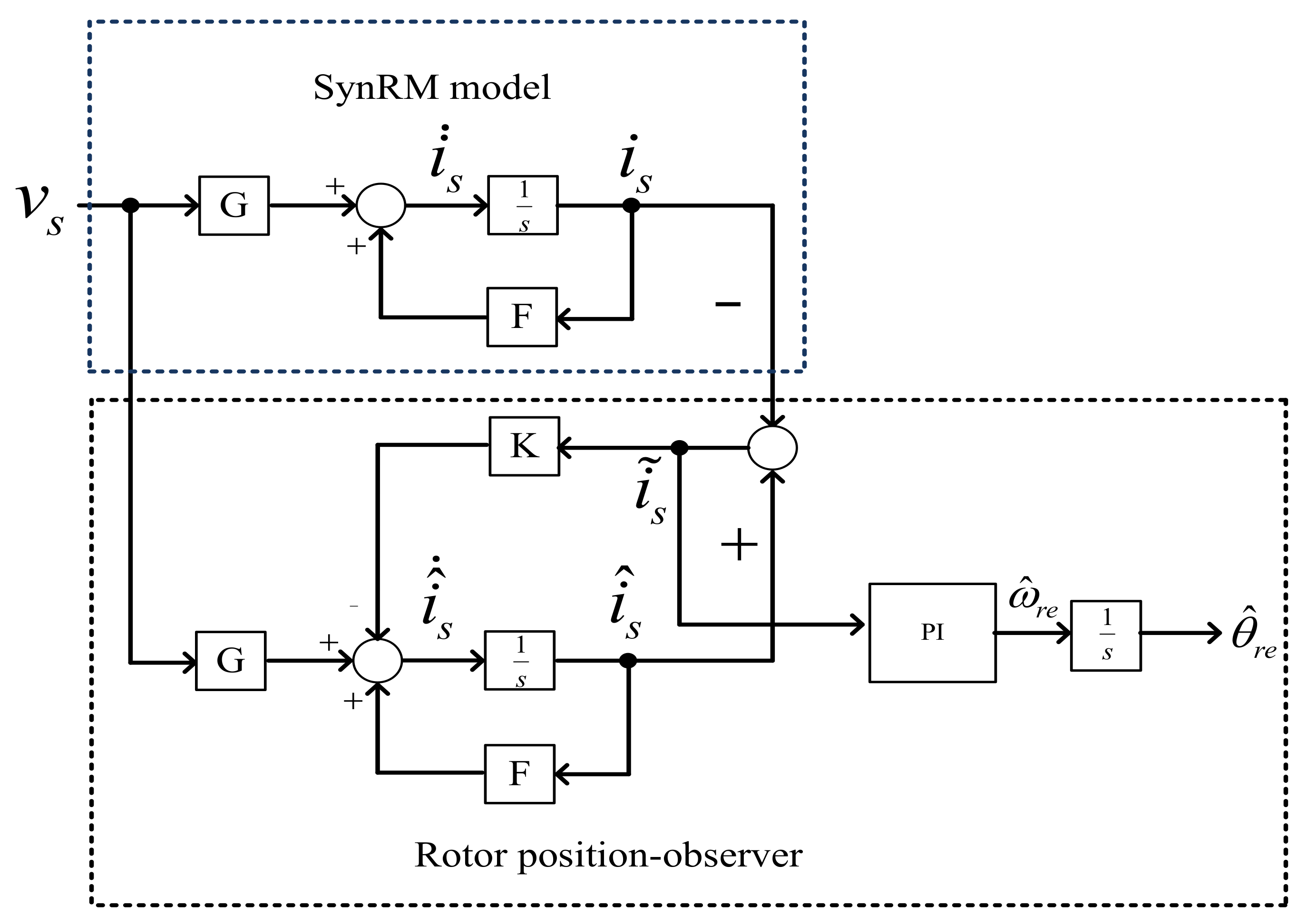
3. Rotor-Position-Observer Design

In this paper, a closed-loop state estimator was derived on the basis of the d-q axis synchronous frame. From Equations (1) and (2), the following differential equation of the d-q axis currents could be derived as follows:

$$\frac{d{i}_s}{dt}=F{i}_s+G{v}_s$$

(6)

In Equation (6), the related vectors and matrices are defined as

$$F=\left[\begin{array}{cc}-\frac{r_s}{L_d}& {\omega }_{re}\frac{L_q}{L_d}\\ -{\omega }_{re}\frac{L_d}{L_q}& -\frac{r_s}{L_q}\end{array}\right]$$

(7)

$$G=\left[\begin{array}{cc}\frac{1}{L_d}& 0\\ 0& \frac{1}{L_q}\end{array}\right]$$

(8)

and

$$v_s=\left[\begin{array}{c}{v}_d\\ v_q\end{array}\right],$$

(9)

where F and G are matrices, and $i_s$ and $v_s$ are current and voltage vectors. Figure 3 shows the proposed closed-loop observer that can be described as follows [11,12]:

$$\frac{d{\widehat{i}}_s}{dt}=F{\widehat{i}}_s+G{v}_s-K({\widehat{i}}_s-i_s)=F{\widehat{i}}_s+G{v}_s-K{\tilde{i}}_s.$$

(10)

From Equation (10), one can define the related vectors and matrix as follows:

$$K=\left[\begin{array}{cc}{k}_1& 0\\ 0& k_2\end{array}\right]$$

(11)

and

$${\widehat{i}}_s=\left[\begin{array}{c}{\widehat{i}}_{ds}\\ {\widehat{i}}_{qs}\end{array}\right],$$

(12)

where ${\widehat{i}}_{ds}$ and ${\widehat{i}}_{qs}$ are the estimated d-q axis currents, ${\tilde{i}}_s$ is the estimated current vector, and K, including $k_1$ and $k_2$, is the gain matrix of the proposed observer. From Equation (10) and Figure 3, one can understand that a different matrix K can be designed to determine the converging rate of estimated current vector, ${\widehat{i}}_s$ for different speeds. Detailed analysis is shown as follows.

First, from Equations (10) and (6), one can obtain the current vector error as follows:

$$\frac{d{\tilde{i}}_s}{dt}=F{\tilde{i}}_s-K{\tilde{i}}_s.$$

(13)

From Equation (13), the equation can be rewritten as follows:

$$\frac{d{\tilde{i}}_s}{dt}=M{\tilde{i}}_s$$

(14)

and

$$M=F-K=\left[\begin{array}{cc}-\frac{r_s}{L_{ds}}& {\omega }_{re}\frac{L_{qs}}{L_{ds}}\\ -{\omega }_{re}\frac{L_{ds}}{L_{qs}}& -\frac{r_s}{L_{qs}}\end{array}\right]-\left[\begin{array}{cc}{k}_1& 0\\ 0& k_2\end{array}\right]=\left[\begin{array}{cc}-\frac{r_s}{L_{ds}}-k_1& {\omega }_{re}\frac{L_{qs}}{L_{ds}}\\ -{\omega }_{re}\frac{L_{ds}}{L_{qs}}& -\frac{r_s}{L_{qs}}-k_2\end{array}\right]$$

(15)

The eigenvalues of matrix M can be derived as follows:

$$\begin{array}{c}\\ \det (\lambda I-M)={\lambda }^2+(\frac{r_s}{L_{qs}}+\frac{r_s}{L_{ds}}+k_1+k_2)\lambda +\frac{r_s{}^2}{L_{ds}{L}_{qs}}+\frac{r_s}{L_{ds}}{k}_2+\frac{r_s}{L_{qs}}{k}_1+k_1{k}_2+{\omega }_{re}{}^2\\ \hspace{0.17em}\hspace{0.17em}\hspace{0.17em}\\ =0\end{array}$$

(16)

The two eigenvalues $\alpha$ and $\beta$ of the $\det (\lambda I-M)$ are expressed as

$$\alpha ,\beta =-\frac{(\frac{r_s}{L_{qs}}+\frac{r_s}{L_{ds}}+k_1+k_2)}{2}\pm \frac{\begin{array}{l}\sqrt{{(\frac{r_s}{L_{qs}}+\frac{r_s}{L_{ds}}+k_1+k_2)}^2-4\left(\frac{r_s{}^2}{L_{ds}{L}_{qs}}+\frac{r_s}{L_{ds}}{k}_2+\frac{r_s}{L_{qs}}{k}_1+k_1{k}_2+{\omega }_{re}{}^2\right)}\end{array}}{2}$$

(17)

Assuming estimated current vector ${\tilde{i}}_s$ has two poles, which are $-\alpha$ and $-\beta$, the following equation exists and can be described as

$$(\lambda +\alpha )(\lambda +\beta )=0.$$

(18)

From Equation (18), one can obtain

$${\lambda }^2+(\alpha +\beta )\lambda +\alpha \beta =0.$$

(19)

Comparing Equations (16) and (19), one can derive

$$(\alpha +\beta )=\frac{r_s}{L_{qs}}+\frac{r_s}{L_{ds}}+k_1+k_2$$

(20)

and

$$\alpha \beta =\frac{r_s{}^2}{L_{ds}{L}_{qs}}+\frac{r_s}{L_{ds}}{k}_2+\frac{r_s}{L_{qs}}{k}_1+k_1{k}_2+{\omega }_{re}{}^2$$

(21)

One can assign the two different negative poles,$-\alpha$ and $-\beta$, in Equations (20) and (21), at different operating speeds. As a result, the proposed SynRM drive system had similar dynamic responses for q-axis current errors at different operating speeds. Moreover, a Lyapunov function candidate $V$ can be defined as

$$V={\tilde{i}}_s{}^T{\tilde{i}}_s.$$

(22)

From Equation (22), $V$ has a positive definite value. Because $M^T$ and M are negative definite matrices, the differential value of the Lyapunov is expressed as follows [18,19,20]:

$$\stackrel{•}{V}={\tilde{i}}_s{}^T(M^T+M){\tilde{i}}_s<0$$

(23)

Equation (23) shows that current error vector ${\tilde{i}}_s$ asymptotically converges and reaches zero at a steady state. The ${\tilde{\omega }}_{re}$ is defined as

$${\tilde{\omega }}_{re}={\widehat{\omega }}_{re}-{\omega }_{re},$$

(24)

where ${\widehat{\omega }}_{re}$ is the estimated speed, and ${\tilde{\omega }}_{re}$ is the estimated speed error. From Equation (24) and [7,8], one can use ${\tilde{i}}_q$ to replace current vector error ${\tilde{i}}_s$ and obtain the following equation:

$${\widehat{\omega }}_{re}(t)=K_P{\tilde{i}}_q+K_I{{\displaystyle {\int }_{t_0}^t{\tilde{i}}_q}}_{}d\tau +{\widehat{\omega }}_{re}(t_0)$$

(25)

where ${\widehat{\omega }}_{re}(t_0)$ is the initial estimated speed, $t_0$ is the initial value of time, t is the value of the current time, and $\tau$ is the variable. Finally, estimated rotor position ${\widehat{\theta }}_{re}(t)$ is

$${\widehat{\theta }}_{re}(t)={\displaystyle {\int }_{t_0}^t{\widehat{\omega }}_{re}}d\tau +{\widehat{\theta }}_{re}(t_0)$$

(26)

After digitizing Equations (25) and (26), one can obtain estimated electrical-rotor speed ${\widehat{\omega }}_{re}(m)$ and rotor position ${\widehat{\theta }}_{re}(m)$ as follows:

$${\widehat{\omega }}_{re}(m)=K_P{\tilde{i}}_q(m)+K_I{\displaystyle \sum _{n=1}^m{\tilde{i}}_q(n)}\Delta t$$

(27)

and

$${\widehat{\theta }}_{re}(m)={\displaystyle \sum _{n=1}^m{\widehat{\omega }}_{re}(n)}\Delta t+{\widehat{\theta }}_{re}(0),$$

(28)

where ${\widehat{\theta }}_{re}(0)$ is the initial estimated position and n is the iterative number. The proposed position observer is illustrated in Figure 3. First, the current vector observer of the ${\widehat{i}}_s$ was constructed. Next, the error of the current vector observer,${\tilde{i}}_s$, was computed. After that, motor-speed observer ${\widehat{\omega }}_{re}$ was obtained via proportional-integral (PI) controller. Finally, motor-position observer ${\widehat{\theta }}_{re}$ was computed via an integral controller.

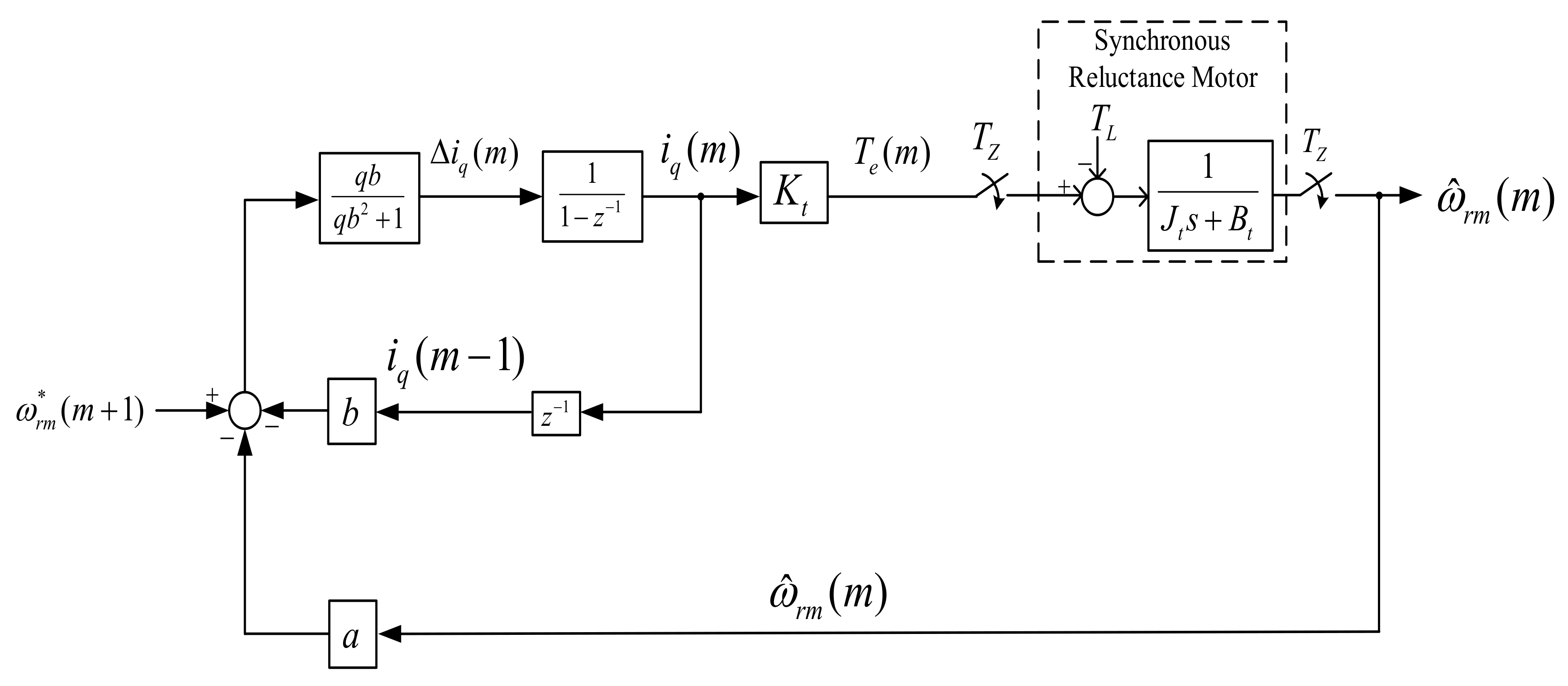
4. Predictive-Controller Design

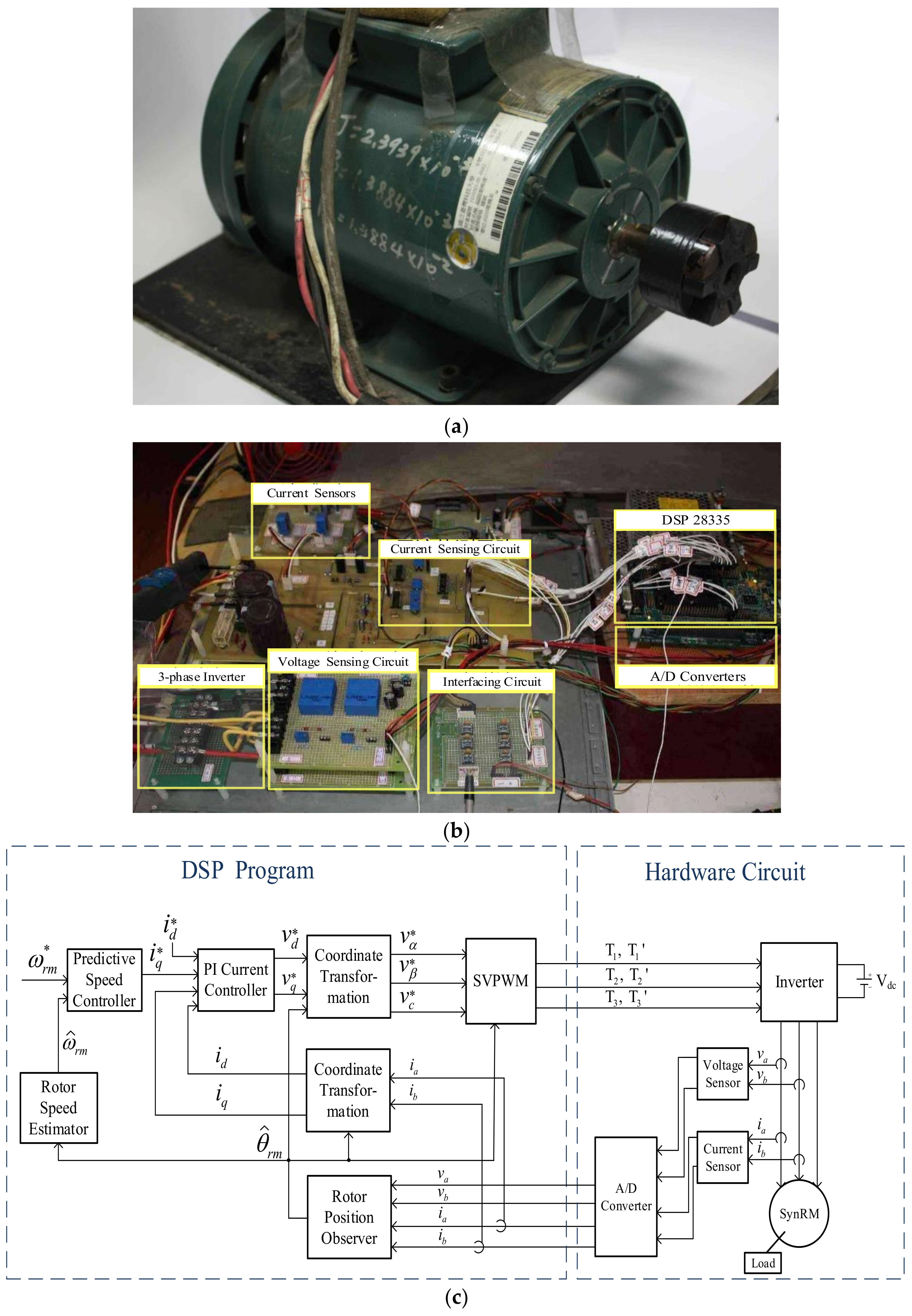
Predictive control is a new control technique that has had strong and widespread impact on industrial applications [20]. It has been used in process control, transportation control, and robotic control for more than three decades. Because of the powerful computation ability of digital-signal processors (DSPs), predictive control has been widely utilized for power converters and motor drives [21,22]. In our paper, predictive control was used for the first time for a sensorless SynRM drive.

The continuous-time dynamic equation of the speed of the SynRM without an external load is

$$\frac{d{\omega }_{rm}}{dt}=\frac{1}{J_t}(T_e-B_t{\omega }_{rm})$$

(29)

Combining Equations (3) and (29), one can obtain:

$$\frac{{\omega }_{rm}^{}(s)}{i_q^{}(s)}=G_c(s)=\frac{K_t^{}}{J_t^{}s+B_t^{}},$$

(30)

where ${\omega }_{rm}^{}(s)$ is mechanical-motor speed, $G_c(s)$ is the transfer function of the uncontrolled plant, and $J_t$ and $B_t$ are the inertia of the motor and the viscous frictional coefficient of the motor, respectively. After inserting a zero-order-hold device in front of transfer function $G_c(s)$, transfer function $G_d(s)$ can be rewritten as

$$G_d^{}(s)=H(s)G_c^{}(s)=\frac{1-e_{}^{-s{T}_z^{}}}{s}\cdot \frac{K_t^{}/J_t^{}}{s+(B_t^{}/J_t^{})}.$$

(31)

By converting the continuous into the discrete domain, discrete transfer function $G_d(z)$ is

$$\begin{array}{l}{G}_d^{}(z)=\frac{{\omega }_r(z)}{i_q(z)}\\ \hspace{0.17em}\hspace{0.17em}\hspace{0.17em}\hspace{0.17em}\hspace{0.17em}\hspace{0.17em}\hspace{0.17em}\hspace{0.17em}\hspace{0.17em}\hspace{0.17em}\hspace{0.17em}\hspace{0.17em}\hspace{0.17em}=\frac{K_{}^{}}{B_t^{}}\cdot \frac{(1-e_{}^{-\frac{B_t^{}}{J_t^{}}{T}_z^{}}{)\mathrm{z}}_{}^{-1}}{(1-e_{}^{-\frac{B_t^{}}{J_t^{}}{T}_z^{}}{\mathrm{z}}_{}^{-1})}\end{array}$$

(32)

From Equation (32), one can obtain the discrete-time dynamic speed equation as

$${\omega }_{rm}^{}(m+1)=a{\omega }_{rm}^{}(m)+b{i}_q^{}(m),$$

(33)

where m is the sampling step of the digital control system. In Equation (33), parameters are shown as

$$a=e_{}^{-\frac{B_t^{}}{J_t^{}}{T}_z^{}}$$

(34)

and

$$b=\frac{K_t^{}}{B_t^{}}\left(1-e_{}^{-\frac{B_t^{}}{J_t^{}}{T}_z^{}}\right).$$

(35)

To simplify the computations of the DSP in this paper, the predictive horizon and control horizon were selected as 1. Performance index $J_p(m)$ was defined in previous research as follows [21,22]:

$$J_p(m)=q{\left[{\omega }_{rm}^{}(m+1)-{\omega }_{rm}^{*}(m+1)\right]}^2+{\left[\Delta i_q(m)\right]}^2,$$

(36)

where q is a weighting factor. To prevent the positive speed error from canceling the negative speed error, or the positive control input from canceling the negative control input, we selected the square of the speed error and control input as the performance index. By taking the derivative of $J_p(m)$ to $\Delta i_q(m)$, one can obtain the following equation:

$$\frac{\partial J_p(m)}{\partial \Delta i_q(m)}=2qb\left[{\omega }_{rm}^{}(m+1)-{\omega }_{rm}^{*}(m+1)\right]+2\left[\Delta i_q(m)\right]=0$$

(37)

From Equation (37), the q-axis difference is obtained as

$$\Delta i_q(m)=\frac{qb}{q{b}^2+1}\left[{\omega }_{rm}^{*}(m+1)-a{\omega }_{rm}^{}(m)-b{i}_q^{}(m-1)\right]$$

(38)

Ultimately, the optimal q-axis current is derived as follows:

$$i_q(m)=\Delta i_q(m)+i_q(m-1)$$

(39)

From Equations (38) and (39), one can construct a block diagram as demonstrated in Figure 4.

5. Implementation

To evaluate the theoretical analysis and simulated results, a SynRM sensorless drive system was implemented. The synchronous reluctance motor, type P56H5012, manufactured in the United States, is shown in Figure 5a. Figure 5b demonstrates the implemented hardware circuit board. The circuit was a three-phase inverter using six IGBTs, type PS 21265-P/AP, as its power devices. The power devices were used for providing voltages and currents to the motor. The inverter employed space-vector modulation with a 10 kHz switching frequency. In addition, the circuit consisted of voltage- and current-sensing circuits, 12-bit A/D converters, which converted analog signals to digital signals, an interfacing circuit, and a DSP that was a control center. Two Hall effect sensors, type LTS25-NP, manufactured in Switzerland, were used as current sensors. A protecting circuit was utilized to prevent an overload of the SynRM drive system. All hardware circuits were designed by us. The block diagram of the implemented drive system is demonstrated in Figure 5c. First, the voltages and currents were read by the DSP via A/D converters. Next, the DSP executed the algorithms of the position observer to obtain the estimated rotor position and speed. The DSP compared the speed command and the estimated speed to compute the q-axis command. After that, the DSP used the PI control to obtain the voltage commands. Then, the DSP used the d-q to an a-b-c axis for coordinate transformation and to compute the three-phase voltage commands. Finally, the DSP sent triggering signals $T_1$ to $T_3{}^{\prime }$ to the inverter.

A DSP, type TMS-320F-28335 [23], manufactured in the USA, was used as a computation tool to execute the position-estimating algorithm and predictive-control algorithm. The sampling time of the current-loop was 100 $\mathsf{\mu }s$, and the speed loop was 1 ms. The d-axis current command was set at 0.5 A to provide the required flux linkage. A larger d-axis current command increased the output torque; however, it also created flux saturation. The q-axis was also adjusted to obtain a quick torque response. Then, the proposed position observer was used to compute the rotor position.

A dynamometer, type TM-5MT(DS), made by Neiwa Company, was used for adding an external load to the SynRM. A power supply was utilized to provide 320 V to the inverter. The motor used in this paper was a three-phase, four-pole, 220 V, 560 W, 3.4 A, 60 Hz, 1800 rpm, Y-connected SynRM. Its parameters were as follows:

Stator resistance $r_s$ was 2 $\Omega$; d-axis inductance $L_d$ was 148 mH; q-axis inductance $L_q$ was 67.2 mH; interia, $J_t$ was 0.0024 kg.m${}^2$; and friction coefficient $B_t$ was 0.0015 N.m/(rad/sec).

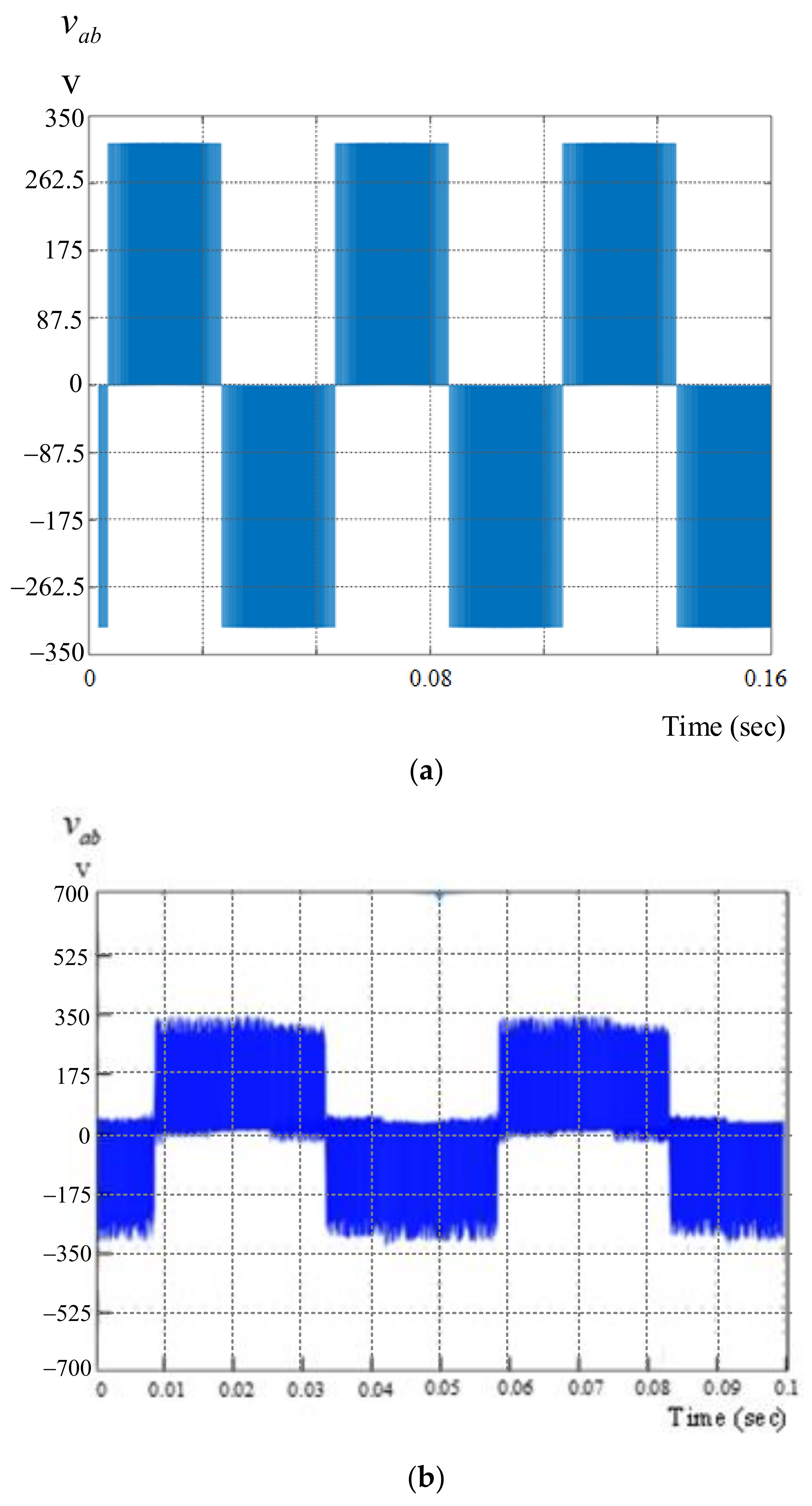
6. Experiment Results

To evaluate the proposed methods, several results are illustrated in this paper. Input DC voltage was 320 V, the sampling time of the speed-loop control was 1 ms, and the current loop was 100 $\mathsf{\mu }s$. The predictive speed control chose one step as the prediction and control horizons. PI speed controller parameters were determined by pole assignment, which were near $P_1=-2+j0.5$ and $P_2=-2-j0.5$. After that, one could obtain $K_P=45$ and $K_I=4$, and the d-axis current command was 0.5 A. The parameters of the PI controller of the current loop were determined by pole assignment, which uses a similar method as the PI controller of the speed loop.

Figure 6a demonstrates simulated line voltage $v_{ab}$. The line voltage was a pulse-width modulation (PWM) modulated voltage waveform with a 10 kHz switching frequency. Figure 6b shows measured line–line voltage $v_{ab}$. Both simulated and measured voltages were very close. In addition, the line–line voltage had positive and negative voltages sequentially because the space-vector pulse-width modulation (SVPWM) was applied. Figure 7a displays the simulated a-phase current, Figure 7b displays the measured a-phase current, and both currents were near-sinusoidal waveforms. Figure 7c displays the measured a-phase current harmonics. Figure 8a illustrates the comparison of the simulated results of the real and estimated rotor positions. Figure 8b illustrates the comparison of the measured results of the rotor positions. Figure 8c illustrates the measured estimated position error, which was between 0 and 4 electrical degrees. The estimated position error had a nonrepetitive waveform due to the influence of the PI controllers, which is shown in Figure 3. Figure 9a,b shows the q-axis current errors at operating speeds of 1100 and 1800 rpm, and the q-axis current errors had similar dynamic responses. The main reason was that similar poles were assigned for different speeds in this paper. In addition, the q-axis estimated current,${\tilde{i}}_q$, could reach zero at both operating speeds. Figure 10a,b illustrates the simulated and measured lowest operating speeds, which were 30 rpm. The SynRM drive system had obvious torque pulsations when it was operated below 30 rpm. Figure 11a,b illustrates the highest speeds at 1800 rpm, and they had similar transient responses. Figure 12a shows the simulated disturbance responses at 500 rpm and 2 N.m, and Figure 12b shows the measured load-disturbance responses in the same situation. The simulated and measured results were similar. The predictive speed controller performed better, including quicker recovery time and lower speed drop, than the PI controller. Figure 13a demonstrates the simulated responses, which reversed repeatedly between 200 and −200 rpm. Figure 13b demonstrates the measured responses under the same circumstances, and they had similar responses. However, the PI controller had an obvious time delay due to the influence of the integral parameter. Figure 14a demonstrates the simulated results of the triangular tracking responses, and Figure 14b demonstrates the measured results of the triangular tracking responses. The speed of the predictive controller could follow the speed command well. The PI controller, however, caused an obvious phase leg between its commands and speed responses. By choosing proper PI value coefficients, error in waveforms for Figure 12, Figure 13 and Figure 14 could be minimized. However, the tuning of PI controllers relied on trial and error. In addition, each operation point required one parameter set of PI controller. Once the operation point changed, the PI controller could not work well. In this paper, the predictive controller provides a systemic design procedure. By suitably choosing weighting factor q, a systematic controller, which is illustrated in Equations (38) and (39), could be uniquely obtained, and the predictive controller parameters were related to the motor parameters, sampling time, and feedback speed.

7. Conclusions

In this study, a position observer and a predictive controller for a SynRM were simulated and implemented. On the basis of the pole-assignment method, the error dynamics of the q-axis currents had similar poles and close dynamic responses. Both q-axis current errors and rotor-position observer errors could be converged in 2 s. In addition, the measured position errors of the position observer could be within four electrical degrees. Compared to previous research [11], which required a full-order observer to obtain the motor position, this paper provided a simplified method with satisfactory performance, including quick converging time and small steady-state estimation errors. In addition, the DSP computation time of the position observer in this paper was shorter than that in previous research. Furthermore, this paper proposed an original idea that combines the advanced position observer and speed-loop predictive controller for a SynRM drive system.

Experiment results demonstrated that the adjustable range of the SynRM was between 30 and 1800 rpm. Furthermore, the measured results demonstrated that the proposed rotor observer had errors below four electrical degrees, and the predictive controller had better dynamic responses than those of PI controllers. Most of the functions of the predictive controller and position observer were implemented by the DSP; therefore, the proposed synRM drive system uses simple hardware circuits that can easily be applied in industry.

References

1. Bolognani, S.; Ortombina, L.; Tinazzi, F.; Zigliotto, M. Model sensitivity of fundamental-frequency-based position estimators for sensorless PM and reluctance synchronous motor drives. IEEE Trans. Ind. Electron. 2018, 65, 77–85. [Google Scholar] [CrossRef]
2. Wei, M.Y.; Liu, T.H. A high-performance sensorless position control system of a synchronous reluctance motor using dual current-slope estimating technique. IEEE Trans. Ind. Electron. 2012, 59, 3411–3426. [Google Scholar]
3. Varatharajan, A.; Pellegrino, G. Sensorless synchronous reluctance motor drives: A general adaptive projection vector approach for position estimation. IEEE Trans. Ind. Appl. 2020, 56, 1495–1504. [Google Scholar] [CrossRef]
4. Tornello, L.D.; Scelba, G.; Scarcella, G.; Cacciato, M.; Testa, A.; Foti, S.; Caro, S.D.; Pulvirenti, M. Combined rotor-position estimation and temperature monitoring in sensorless, synchronous reluctance motor drives. IEEE Trans. Ind. Appl. 2019, 55, 3851–3862. [Google Scholar] [CrossRef]
5. Senjyu, T.; Shingaki, T.; Uezato, K. Sensorless vector control of synchronous reluctance motors with disturbance torque observer. IEEE. Trans. Ind. Electron. 2001, 48, 402–407. [Google Scholar] [CrossRef]
6. Lim, H.B.; Lee, J.H. The evaluation of online observer system of synchronous reluctance motor using a coupled transient FEM and Preisach model. IEEE Trans. Magnet. 2008, 44, 4139–4142. [Google Scholar]
7. Vagati, A.; Pastorelli, M.; Franceschini, G.; Drogoreanu, V. Flux-observer-based high-performance control of synchronous reluctance motors by including cross saturation. IEEE Trans. Ind. Appl. 1999, 35, 597–605. [Google Scholar] [CrossRef]
8. Tuovinen, T.; Hinkkanen, M. Adaptive full-order observer with high-frequency signal injection for synchronous reluctance motor drives. IEEE J. Emerg. Select. Top. Power Electron. 2014, 2, 181–189. [Google Scholar] [CrossRef] [Green Version]
9. Tuovinen, T.; Hinkkanen, M.; Luomi, J. Analysis and design of a position observer with resistance adaption for synchronous reluctance motor drives. IEEE Trans. Ind. Appl. 2013, 49, 66–73. [Google Scholar] [CrossRef] [Green Version]
10. Tuovinen, T.; Hinkkanen, M. Signal-injection-assisted full-order observer with parameter adaption for synchronous reluctance motor drives. IEEE Trans. Ind. Appl. 2014, 50, 3392–3402. [Google Scholar] [CrossRef] [Green Version]
11. Awon, H.A.A.; Tuovinen, T.; Saarakkala, S.E.; Hinkkanen, M. Discreet-time observer design for synchronous reluctance motor drives. IEEE Trans. Ind. Appl. 2016, 52, 3968–3979. [Google Scholar] [CrossRef]
12. Tuovinen, T.; Hinkkanen, M. Comparison of a reduced-order observer and a full-order observer for sensorless synchronous motor drives. IEEE Trans. Ind. Appl. 2012, 48, 1959–1967. [Google Scholar] [CrossRef] [Green Version]
13. Lin, C.K.; Yu, J.T.; Lai, Y.S.; Yu, H.C. Improved model-free predictive current control for synchronous reluctance motor drives. IEEE Trans. Ind. Electron. 2016, 63, 3942–3953. [Google Scholar] [CrossRef]
14. Hadla, H.; Cruz, S. Predictive stator flux and load angle control of synchronous reluctance motor drives operating in a wide speed range. IEEE Trans. Ind. Electron. 2017, 64, 6950–6959. [Google Scholar] [CrossRef] [Green Version]
15. Carlet, P.G.; Tinazzi, F.; Bolognani, S.; Zigliotto, M. An effective model-free predictive current control for synchronous reluctance motor drives. IEEE Trans. Ind. Appl. 2019, 55, 3781–3790. [Google Scholar] [CrossRef] [Green Version]
16. Antonello, R.; Carraro, M.; Peretti, L.; Zigliotto, M. Hierarchical scaled-states direct predictive control of synchronous reluctance motor drives. IEEE Trans. Ind. Electron. 2016, 63, 5176–5185. [Google Scholar] [CrossRef]
17. Lin, C.K.; Yu, J.T.; Lai, Y.S.; Yu, H.C.; Peng, C.I. Two-vector-based modeless predictive current control for four-switch inverter-fed synchronous reluctance motors emulating the six-switch inverter operation. IEEE Trans. Electron. Lett. 2016, 52, 1244–1246. [Google Scholar] [CrossRef]
18. Ioannou, P.; Fidan, B. Adaptive Control Tutorial; SIAM: Philadelphia, PA, USA, 2006. [Google Scholar]
19. Astrom, K.J.; Wittenmark, B. Adaptive Control, 2nd ed.; Addison-Wesly: New York, NY, USA, 1995. [Google Scholar]
20. Maciejowski, J.M. Predictive Control with Constraints; Pearson Education Limited: London, UK, 2002. [Google Scholar]
21. Rodriquez, J.; Corts, P. Predictive Control of Power Converters and Electrical Drives; Wiley: London, UK, 2012. [Google Scholar]
22. Wang, L.; Chai, S.; Yoo, D.; Gan, L.; Ng, K. PID and Predictive Control of Electrical Drives and Power Converters Using MATLAB/Simulink; Wiley: Singapore, 2015. [Google Scholar]
23. Toliyat, H.A.; Campbell, S. DSP-Based Electromechanical Motion Control; CRC Press: New York, NY, USA, 2003. [Google Scholar]
Figure 1. Synchronous-reluctance-motor (SynRM) structure.
Energies 13 02712 g001
Figure 2. Block diagram of simplified SynRM.
Energies 13 02712 g002
Figure 3. Proposed position observer.
Energies 13 02712 g003
Figure 4. Block diagram of predictive speed control.
Energies 13 02712 g004
Figure 5. Implemented system. (a) Motor; (b) circuits; (c) block diagram.
Energies 13 02712 g005
Figure 6. Line–line voltage of motor. (a) Simulated; (b) measured.
Energies 13 02712 g006
Figure 7. Phase currents. (a) Simulated; (b) measured; (c) harmonics.
Energies 13 02712 g007
Figure 8. Responses at 500 rpm. (a) Simulated position; (b) measured position; (c) measured estimated error.
Energies 13 02712 g008
Figure 9. Measured dynamic q-axis current errors at (a) 1100 and (b) 1800 rpm.
Energies 13 02712 g009
Figure 10. Lowest step-input speed at 30 rpm. (a) Simulated; (b) measured.
Energies 13 02712 g010aEnergies 13 02712 g010b
Figure 11. Highest step-input speed responses at 1800 rpm. (a) Simulated; (b) measured.
Energies 13 02712 g011
Figure 12. 2 N.m disturbance responses (a) simulated (b) measured.
Energies 13 02712 g012
Figure 13. Square-wave tracking responses using different controllers. (a) Simulated; (b) measured.
Energies 13 02712 g013aEnergies 13 02712 g013b
Figure 14. Triangular tracking responses using different controllers. (a) Simulated; (b) measured.
Energies 13 02712 g014