HousEEC: Day-Ahead Household Electrical Energy Consumption Forecasting Using Deep Learning

Abstract

Short-term load forecasting is integral to the energy planning sector. Various techniques have been employed to achieve effective operation of power systems and efficient market management. We present a scalable system for day-ahead household electrical energy consumption forecasting, named HousEEC. The proposed forecasting method is based on a deep residual neural network, and integrates multiple sources of information by extracting features from (i) contextual data (weather, calendar), and (ii) the historical load of the particular household and all households present in the dataset. Additionally, we compute novel domain-specific time-series features that allow the system to better model the pattern of energy consumption of the household. The experimental analysis and evaluation were performed on one of the most extensive datasets for household electrical energy consumption, Pecan Street, containing almost four years of data. Multiple test cases show that the proposed model provides accurate load forecasting results, achieving a root-mean-square error score of 0.44 kWh and mean absolute error score of 0.23 kWh, for short-term load forecasting for 300 households. The analysis showed that, for hourly forecasting, our model had 8% error (22 kWh), which is 4 percentage points better than the benchmark model. The daily analysis showed that our model had 2% error (131 kWh), which is significantly less compared to the benchmark model, with 6% error (360 kWh).

1. Introduction

Electrical energy (EE) is one of the most significant driving forces of economic development, and is considered essential to daily life. Although EE is a clean form of energy when it is used, the production and transmission of electricity can have a negative effect on the environment. Additionally, overproduction of EE is problematic, because storing excess electricity is challenging and difficult even with today’s technological advances. Hence, a system that can accurately predict EE consumption can be used for electricity production planning, and significantly reduce the problems with storage and overproduction.

In recent years, with the introduction of deregulation and liberalization of the energy markets, EE consumption forecasting has become even more relevant. An accurate short-term load forecasting (STLF) system can play a crucial role in effective power system operation and efficient market management. Such a system has multiple benefits: (i) it can optimize the production process, thus reducing the cost of overproduction and improving equipment utilization; (ii) it is eco-friendly, with fewer resources used to produce electricity; (iii) it can help in optimizing power grid load and strengthening reliability; (iv) it can potentially decrease EE consumption costs for households by better planning the production/buying of EE in advance; and (v) it emphasizes EE trading possibilities.

The massive development of smart grid technologies in the residential sector brings many challenges to the load forecasting community. It allows EE consumption to be obtained in close to real time, and allows extraction of valuable data that both the supply and demand side can use for efficient management of the electricity load network.

In recent years, there have been various data-driven approaches for modeling and forecasting EE consumption. Most of them focus on industrial objects, factories, and companies, and some are more focused on households. Furthermore, some focus on short-term forecasts (hourly, daily) with a small prediction horizon (an hour in advance), and some focus on long-term forecasts (weekly, monthly). The studies that focus on STLF with a large prediction horizon (at least one day ahead) are quite limited. Therefore, in this paper, we present the household electrical energy consumption (HousEEC) forecast system, which provides day-ahead household electrical energy (EE) consumption forecasts, using a deep residual neural network (DRNN) that combines multiple sources of information. The key contributions of the paper are as follows:

• A review of the existing EE consumption approaches and a highlight of their current limitations (Section 2).
• An extensive analysis and evaluation of the Pecan Street dataset, the largest and richest household EE consumption dataset (Section 3).
• A novel deep learning (DL) method with a scalable architecture that can work with different numbers of households. It is based on DRNN and includes multisource feature extraction, regression learning, and forecasting of hourly EE consumption of multiple households one day in advance. The proposed DRNN uses pre-activation residual blocks and separate input branches for different types of features (Section 4).
• Novel domain-specific historical time series, from which numerous time and frequency features are extracted (Section 4). These features give new insight into the time-series dynamics and significantly increase the performance of the forecast models.
• An extensive evaluation of the method, including: (i) a comparison of our proposed method with seven machine learning (ML) algorithms, five deep learning (DL) approaches, and three benchmark/reference approaches; (ii) error analysis of different application scenarios (hourly, daily and monthly EE consumption); and (iii) a comparison of achieved results for household STLF with results from other state-of-the-art approaches (Section 5 and Section 6).
• A practical implementation of the system in a prototype web application, where ML models are deployed and execute the forecasts on a daily basis (Section 7).
• A discussion about the results, the forecasting efficiency and its significance, and potential use of the model in a commercial EE monitoring system (Section 8).

2. Related Work

Selecting a forecasting method depends on multiple factors, including the availability and relevance of historical data, desired prediction accuracy, the forecast horizon, and so forth. In recent years, the STLF problem has been tackled by utilizing various methods, each one characterized by different advantages and disadvantages in terms of training complexity, prediction accuracy, limitations in the forecasting horizon, etc. In general, the related work in STLF can be divided into two categories, depending on the type of user (industrial entities or households) and method used (e.g., statistical, ML, DL).

2.1. Related Methods

With the advent of statistical software packages and artificial intelligence techniques, numerous methods have been proposed to model future EE consumption and improve forecasting performance. These methods can be divided into two categories: conventional statistical methods and methods based on artificial intelligence (AI).

Statistical methods provide explicit mathematical models where the load is represented as a function of several input factors. These were the first used methods, and for years represented the benchmark among systems for STLF. All of these methods, which include smoothing techniques, data extrapolation and curve fitting, assume that the load data have an internal structure. Autoregressive moving average (ARMA) models were among the first used in STLF [1,2,3]. Soon they were replaced by autoregressive integrated moving average (ARIMA) models [4] and seasonal ARIMA models [5] to deal with time variance often exhibited by load consumption profiles. Other examples of statistical methods used in STLF are multiple regression [6], exponential smoothing [7], adoptive load forecasting [8,9] and Kalman filtering [10,11]. The major weakness of these approaches is their assumption of the linearity of the observed system. EE forecasting is a complex multivariable and multidimensional estimation problem, and these methods are not always suitable for finding the nonlinear relationship between the independent influencing variables and the EE consumption.

On the contrary, advanced ML methods are suitable for finding patterns and regularities in the data and use them to forecast future EE consumption. ML based methods have shown great performance in the field of STLF. The most commonly used ML algorithms for STLF are support vector machines (SVM) [12,13], random forest [14,15] and artificial neural networks (ANNs) [16]⁠. However, as shown in numerous studies and in the benchmark Global Energy Forecasting Competition 2012 (GEFCom2012) [17], very often, simple ML methods applied to manually crafted complex features (polynomial and exponential interaction features combining multiple variables) achieve better and more robust performance [18]. These features often use the lagged and recency effect, first introduced in [19]. One of the winning teams [20] at GEFCom2012 used lagged hourly and average daily temperature variables in the competition. They applied a gradient boosting algorithm to learn the dependencies between features and target variables. Another winning team at GEFCom2012 [21] used exponentially smoothed temperature variables. They used generalized additive models and kernel regression for long-term load and medium-term forecasting, and random forests for short-term load forecasting.

Over the past few years, DL has been a subject of intense study in many fields, especially in time-series prediction. Deep neural networks (DNNs) have shown the capability to approximate any complex function with arbitrary precision. In [22], the authors showed that some DNN architectures are able to outperform classical ML approaches in the load forecasting task. The authors of [23] proposed convolutional neural network (CNN), as an effective and accurate approach for household-level load forecasting. They showed that CNN is able to capture short-term trends in load data and that a data-augmentation technique can improve the load forecasting accuracy. Compared with conventional feedforward neural networks, recurrent neural networks (RNNs) have the particular advantage of coping with historical data through a feedback connection. In [24], the authors presented a deep RNN to predict electricity consumption for commercial and residential buildings. As an extension of RNN, long short-term memory (LSTM) networks have been used in the load forecasting field in the last few years [25]. The authors of [26] utilized two types of LSTM networks (standard and encoder-decoder architecture) to make predictions for one household. The authors of [27] proposed enhanced-LSTM for EE consumption forecast of a metropolitan power system in France. Their method takes into account the periodicity characteristic of the load consumption by using multiple sequences of input time lags, and achieves higher performance than a single-sequence LSTM. Moreover, different hybrid architectures have been explored in order to avoid the limitations of individual models. A hybrid approach for STLF is presented in [28], where the authors processed the load signal in parallel with a LSTM and CNN. The features generated by the two networks were then used as input in a fully connected network in charge of forecasting the day-ahead load. The authors of [29] proposed a hybrid model which combines general regression neural network (GRNN), minimal redundancy maximal relevance technique and empirical model decomposition. The efficiency of the model is validated on aggregated load data from a power system in China. It shows higher forecasting accuracy than single GRNN and SVM. In [30], a hybrid method is proposed, which combines LSTM, empirical mode decomposition and similar-days selection to build a prediction architecture for short-term load forecasting. The authors concluded that the robustness of individual methods in the hybrid scheme can be an advantage for the forecasting model.

2.2. Related Studies According to User Type

According to the type of user, EE consumption forecasting approaches can be divided into those that focus on industrial entities (industrial consumption) and those that focus on households (residential consumption). The industrial approaches focus on entities such as factories, enterprises and companies, and have substantial commercial potential because industry consumes significant amounts of EE. STLF for industrial entities in Spain is discussed in [31]. The authors presented a neuro-fuzzy system with a backpropagation learning algorithm and compared the results achieved with those of other techniques, such as multilayer perceptron and statistical ARIMA processes. In [32], the authors present a model for STLF for a hospital in China. They combined LSTM and CNN and explored the network performance by considering coupling of electrical loads, gas and heating. The authors of [33] introduced an ARMA model for load forecasting of industrial companies, with focus on EE consumption profiles where stochastic changes in the regime can be observed. In [34], a set of multiple linear regression models are developed for modeling industrial loads. The data used in the study were collected from an Italian factory. In this study, the authors showed how few qualitive variables characterize the production schedule. In [35], the authors develop different models for forecasting the next hour load using data from a Spanish industrial pole. With an optimized model for single-hour prediction, a hybrid strategy was applied to build a complete day-ahead hourly load forecasting model. In general, the studies related to industrial EE consumption provide more accurate models compared to households, probably because industrial entities have strict regulations (i.e., shifts and working time), which makes the forecasting less challenging.

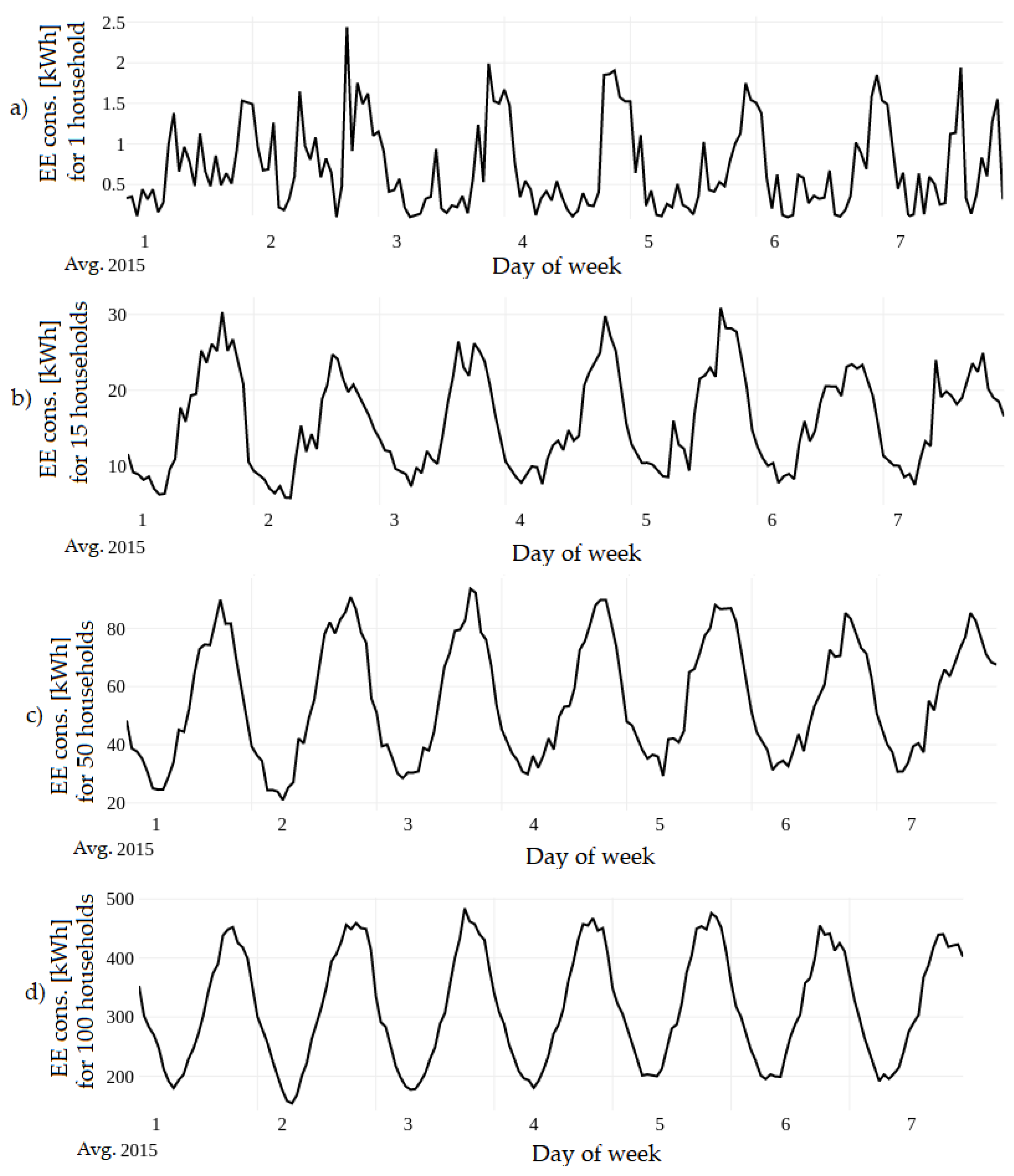
On the other hand, residential EE consumption is more challenging to forecast. Each household has its own pattern and electricity consumption profile, which are determined by the number of occupants, their lifestyle, the household area, electrical appliances present in the household, etc. Additionally, household-level EE consumption can vary considerably from one day to the next due to work schedules, holidays, weather conditions, etc. Therefore, most of the approaches in this field tend to avoid such uncertainty by using load aggregation: they focus on forecasting EE consumption of clusters of households, usually grouped by location (i.e., buildings and neighborhoods). Load aggregation usually reduces the inherent variability in load consumption, which results in smoother load shapes that are more predictable. This effect is illustrated in Figure 1.

In [36], the authors used clustering method to divide different types of households. For each cluster, a neural network is fitted, and their forecasts are added together to form predictions for the aggregated load. The authors demonstrate that clustering significantly increases forecast accuracy. Similarly, in [37], the authors propose a three-step process, consisting of clustering approaches, load forecasting for each cluster, and aggregating the forecasts to obtain results at a system level. The authors of [38] also show that aggregating more households improves the relative forecasting performance. They compare load forecasting accuracy at various levels of aggregation for many forecasting methods. In [39], the load consumption forecasting problem is addressed using random forest and support vector regression (SVR). Predictions are made on three spatial scales, and the obtained results show that combination of K = 32 clusters and random forest yields highest forecasting accuracy.

The systems that focus on neighborhoods lose vital information about each household; thus, they have lower commercial value, i.e., such systems cannot monitor and learn the behavior of individual households. Therefore, they cannot offer personalization and planning of EE consumption, which will be useful for cost reduction. There are just a handful of recent studies covering short-term load forecasts (e.g., day-ahead, hourly) for individual households, since they are still very challenging. The authors of [40] present a pooling-based deep recurrent neural network (PDRNN), which batches groups of customer EE consumption profiles into a pool of inputs. The authors of [41] applied Kalman filtering to single household data for a sampling period and forecast horizon of one hour. In [42], an approach is proposed to model the load of individual households based on daily schedule pattern analysis and context information.

However, the authors focus on predicting consumption with a prediction horizon shorter than one day, which does not have the same economic value as one-day-ahead hourly forecasts. Typically, the results of day-ahead forecast are used as a baseline for planning of the 24 h period of the next day, while forecasts with forecast horizon shorter than one day (intraday forecast) are mostly used for adjustment of day-ahead purchases [43]. Accurate day-ahead forecast minimizes the possibility of overproduction and underproduction, and satisfies load requirements in a more economical way, thus reducing the total operation costs [44].

Our proposed solution for EE consumption forecasting includes short-term forecasting (day-ahead forecast, for each hour of the day separately) for household consumption, which has significant economic and industrial value. In our study, we focus on STLF of individual households, which we believe is very specific and challenging due to the variability in consumption and randomness of households.

3. Dataset

3.1. Pecan Street Dataset

In order to develop a model that can accurately and reliably forecast the EE consumption, we performed a thorough analysis of the existing datasets. We analyzed most of the datasets in this domain and then selected Pecan Street dataset as the most appropriate one for our study. An extensive analysis of other relevant datasets and their characteristics can be found in Appendix A.

The Pecan Street dataset is one of the richest datasets related to residential EE consumption. It consists of EE consumption data, obtained from approximately 1000 households in the USA, mainly Austin, Texas. The dataset contains the actual EE consumption values from each household in one-minute intervals, collected by eGauge devices [45]. Our analysis is based on hourly household EE consumption, given in kilowatt-hours (kWh). Descriptive statistics of the EE consumption are provided in

Table 1. Descriptive statistics of EE consumption.

Number of Samples	Minimum	Maximum	Mean	Standard Deviation	25th Percentile	50th Percentile	75th Percentile
4,832,504	0.001	35.19	1.28	1.32	0.43	0.82	1.66

.

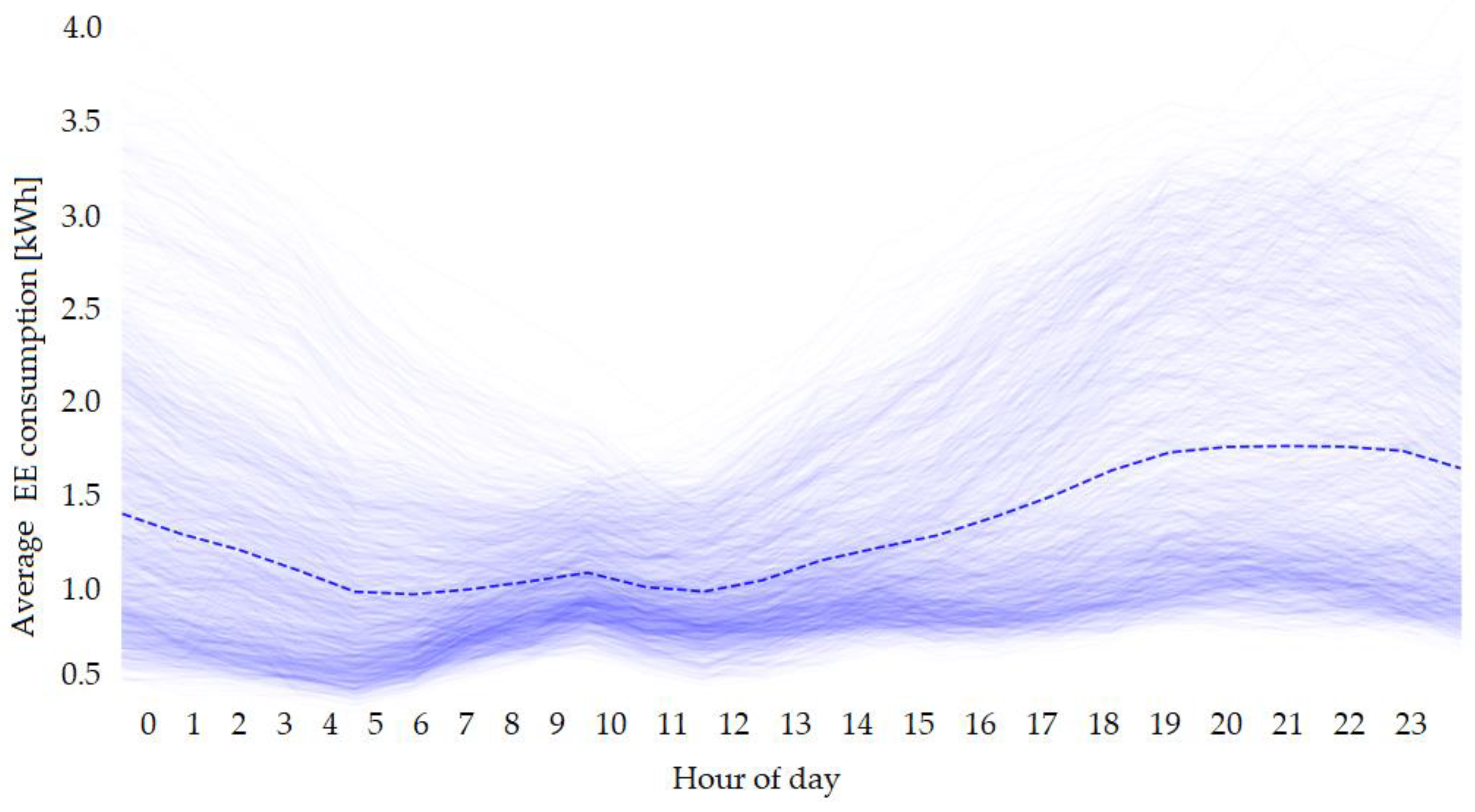
Figure 2 shows the average daily EE consumption, i.e., each line in the figure represents average EE consumption for one day in the dataset. Each line is obtained by averaging the load consumption values for each hour in the day separately. The dashed line represents the mean EE consumption at hourly intervals.

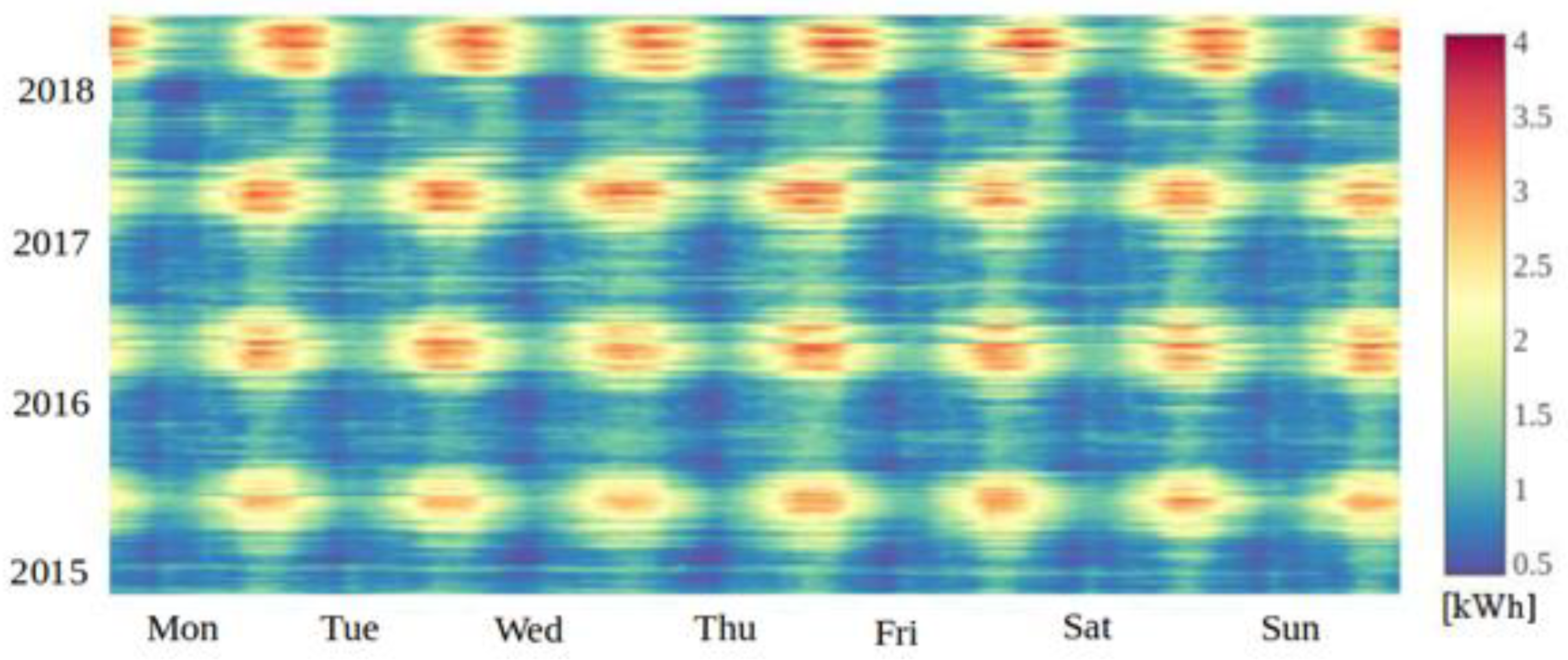
Additionally, the Pecan Street dataset contains extensive weather data for the observed region. STLF is mainly influenced by weather parameters, because heating, ventilation and air-conditioning (HVAC) are highly dependent on outdoor temperature, humidity, wind speed, etc. Figure 3 shows a two-dimensional heatmap of EE consumption. The heatmap represents average hourly consumption in appropriate time intervals with predefined colors, where warmer colors represent higher consumption. Figure 3 shows that there is a noticeable increase in average electricity consumption in the summer months. This is specific to this dataset, i.e., it is collected in Texas, USA, where the summer temperature is significantly high, and there is increased use of air-conditioning. Therefore, the steady increase in EE consumption during the summer months can be attributed to the use of air-conditioners.

The data used in this study were collected from 925 households for a period of almost four years (2015, 2016, 2017, and nine months of 2018). In order to accurately evaluate the proposed forecasting model’s performance, we divided the data into three parts: (i) 27 months were used for training data (6 even-numbered months of 2015, all of 2016, and the first 9 months of 2017). (ii) Six months (odd-numbered months) from 2015 were taken for validation data. (iii) The last 12 months were chosen for test data (last 3 months of 2017 and 9 months of 2018).

3.2. Dataset Preprocessing

One of the most important steps towards developing an accurate ML model is data preprocessing. This process prepares the data for analysis by dealing or removing the data that is incorrect, incomplete, irrelevant, duplicated or improperly formatted. The preprocessing of the dataset included the following steps:

• Handling incorrect values for certain variables—In particular, we encountered instances with negative values for consumed electricity, which is impossible and indicates a mistake. In this case, we were able to calculate the value from other variables available in the dataset. For instance, we calculated the total EE consumption as the sum of consumed power from the solar grid and power drawn from the electrical grid.
• Handling outliers (instances which greatly deviate from the expected range) and missing values—If the outliers or missing values pertained to weather-related variables, the true value could be extracted from other instances referring to the same moment in time. However, in the case that the reported load consumption was incorrect from the start, the particular instance was omitted from the dataset entirely.
• Handling sequential values for EE consumption that are identical—In some situations, the sensors in certain households reported a constant value over a prolonged period of time. In this case, we assumed there was a fault with the sensor. Due to the large number of distinct households in the dataset, we could remove these instances.

4. Methodology

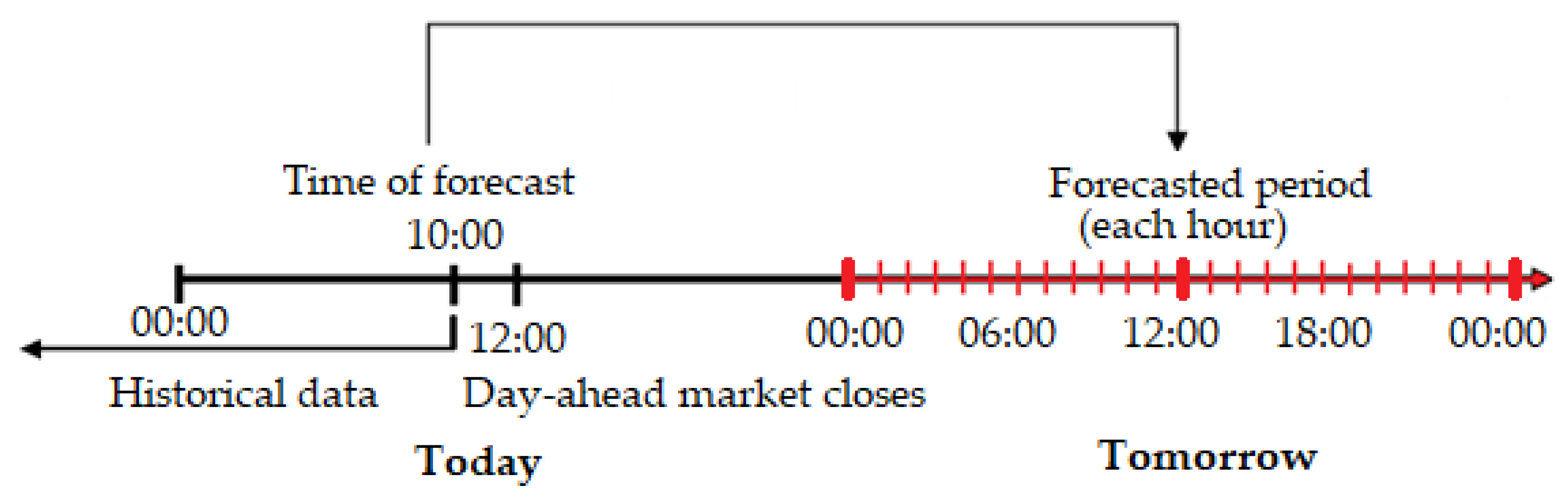
In the day-ahead electricity market, generation companies and retailers submit supply and demand orders for every hour of the following day. Therefore, the focus of our work was to create a model that can forecast electricity consumption one day ahead, at 10:00, for every hour of the following day (shown in Figure 4) [46].

This timeline allows planning of the production for the following day in accordance with the day-ahead electricity market. According to this timeline, we developed two models that make predictions for different hours of the next day: one for the hours from midnight to 09:00, and one for the rest of the day. The main reason for developing two models is that we want to include the 24-h-before load consumption value for the hours from midnight to 09:00, which, at the time when the predictions are made (at 10:00), are only available for these hours. We considered this as valuable additional information that can improve forecasting for the first nine hours of the following day, because the periodic nature of EE consumption makes the most recent EE consumption values the dominant factor in STLF [47].

4.1. Feature Engineering

EE load forecasting is a complex multivariable and multidimensional estimation problem. The impacts of many influencing factors that affect load consumption need to be studied in order to develop a precise load forecasting model. Thus, we extracted several features from multiple sources, which can mainly be grouped into two categories: contextual and historical load features.

4.1.1. Contextual Features

• Weather features

The weather is a crucial driving factor in EE consumption. That is why it is a common EE consumption forecasting practice to include weather variables, such as wind speed, humidity and precipitation intensity, in forecasting models. The factor that has the most influence on EE consumption is temperature. Several weather-related features were extracted, and the main focus was on the temperature-related features.

• Calendar features

The social element is part of the reason for the hourly, daily and weekly patterns in EE consumption [48]. To allow forecast models to take into account the EE consumption variations which are tied to days, times of the day and seasons, we included some calendar data as nominal features. We also included information about the special days according to the area of interest, Austin, Texas.

• Interaction features

We also used interaction features, i.e., combinations of two existing features [49]. The hours in the days of a week may result in different loads due to human activities. For instance, there may be a smaller load on weekend mornings than weekday mornings, because people usually do not get up as early as when they have to go to work. This results in lower EE consumption values. The implementation of this group of features was simply done by multiplying two features.

For a full table with all extracted contextual features, see Appendix B.

4.1.2. Historical Load Features

Load consumption is highly related to historical load, due to its periodic nature. Thus, in this study, historical loads of up to one week were used to predict the day-ahead hourly load.

• Standard features

Due to the strong daily patterns of EE consumption, it is highly correlated to consumption at the same hour of previous days [50,51,52]. That is why the following lagged values were used in the training process of the forecasting model:

• Historical EE consumption values by individual household for particular hours: load_t-24h, load_t-25h, load_t-26h, load_t-48h, load_t-49h, load_t-50h, load_t-72h, load_t-96h, load_t-120h, load_t-144h, and load_t-168h
• Average historical load consumption values from all households for particular hours: avg_load_t-24h, avg_load_t-25h, avg_load_t-26h, avg_load_t-48h, avg_load_t-49h, avg_load_t-50h, avg_load_t-72h, avg_load_t-96h, avg_load_t-120h, avg_load_t-144h, and avg_load_t-168h

Features load_t-24h, load_t-25h and load_t-26h are used only for the first model, for the hours from midnight to 09:00 (see Section 4).

• Domain-specific historical load features

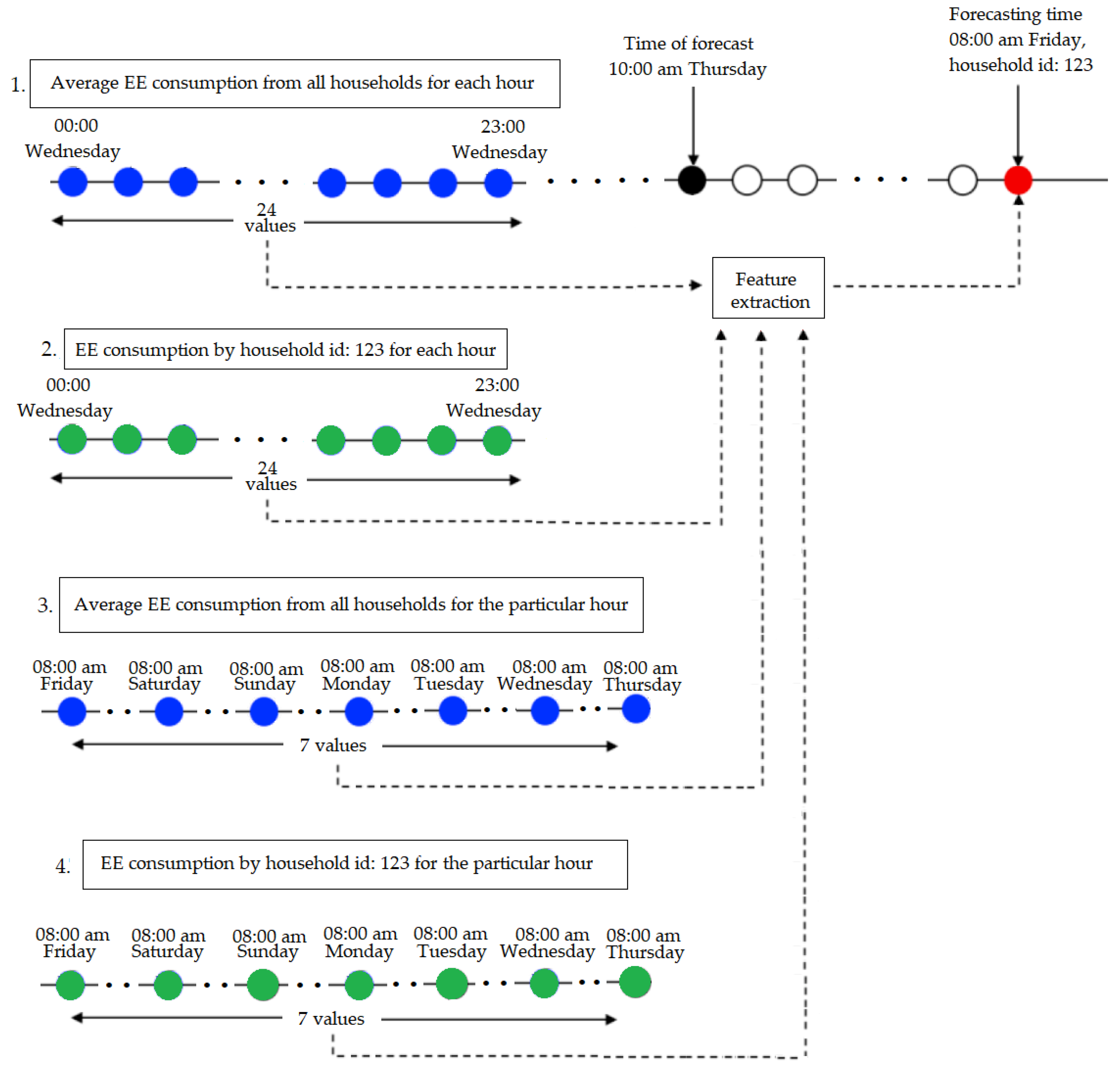
Based on the fact that future EE consumption is highly related to historical load, we additionally analyzed four types of time series. The first two take into account the strong daily pattern of EE consumption, and consist of historical load data from the day previous to the day when the predictions are made (all 24 h): one refers to the average load consumption in each hour, calculated from all households present in the system, and the other refers to the load consumption of each household in the same hours. The other two types of time series take into account the significance of the lagged values of EE consumption related to the same hours of previous days. More specifically, one of these time series consists of average values for load consumption (from all households) from hour 24, 48, 72, 96, 120, 144 and 168 prior to the forecasted hour, and the other consists of load consumption of each household in the same hours. As mentioned before, the 24-h-before EE consumption value is only used for instances referring to the first defined interval (midnight to 09:00). It should be noted that in the previous section, the lagged values of EE consumption were used as actual features, but in this section they are used for constructing time series from which additional time and frequency features will be extracted.

To include valuable characteristics about the manner of EE consumption in the feature vector, for each instance we generated a comprehensive set of features based on these four types of time series. The features were extracted using the TSFRESH (https://tsfresh.readthedocs.io/en/latest/text/list_of_features.html) Python package, which offers extraction of time and frequency domain features from time-series. We generated 400 new features for each instance. These features include minimum, maximum, variance, correlation, covariance, skewness, kurtosis, number of times the signal is above/below its mean, signal mean change, its autocorrelations (correlations for different delays), etc. These new features give new insight into time-series dynamics, and we believe that they can be significant in improving forecast accuracy. Figure 5 shows how the four time series are constructed for a forecast for a particular household at 08:00.

4.2. Deep Residual Neural Network

DL is part of ML, and is based on artificial neural network architecture [53]. DL allows models comprised of numerous processing layers to learn data representations with multiple levels of abstraction. DL architectures have been applied to many fields, where they have produced results comparable, or in some cases superior, to those of human experts.

One type of DNN that was recently proposed is the deep residual neural network (DRNN). This type of deep network has performed extremely well on natural language processing tasks [54,55] and has emerged as a state-of-the-art architecture in computer vision, image segmentation and object detection [56,57] More recently, architectural variants of DRNN have also been used in load forecasting, where they have shown improvement in aggregated load forecast compared to conventional regression models [58,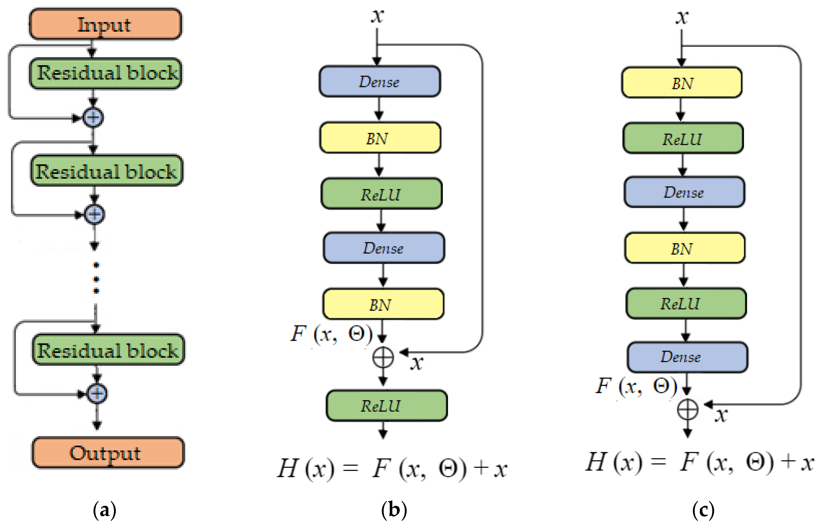59]. Therefore, in this work we further explore the effectiveness of DRNN architecture in day-ahead load forecasting for single households. A DRNN can easily be constructed by stacking several residual blocks (Figure 6a). In the residual block, a mapping from $x$ to $\mathsf{\Theta }$ is learned, where $\mathsf{\Theta }$ is a set of weights related to the residual block. Accordingly, the general representation of the residual block can be written as shown in Equation (1):

$$H\left(x\right)=F\left(x, \mathsf{\Theta }\right)+x.$$

(1)

The forward propagation of the structure, where k residual blocks are stacked, can be represented as shown in Equation (2):

$$x_K=x_0+{\displaystyle \sum }_{i=1}^{K}F\left(x_{i-1}, {\mathsf{\Theta }}_{i-1}\right)$$

(2)

where $x_0$ and $x_K$ are the input and the output of the residual network, respectively, and ${\mathsf{\Theta }}_i={\{\mathsf{\Theta }}_{i,l}| 1 \le l \le L\}$ is the set of weights related to the ith residual block, L being the number of layers within the block. Basically, x has no parameters and only adds the output from the previous layer to the layer ahead. The original structure of a residual block used for building a DRNN is shown in Figure 6b.

As DRNNs gain more and more popularity in the research community, their architecture is more intensely studied. There are many proposed interpretations of DRNN architecture and variants of residual blocks. For our DRNN architecture, we used a pre-activation variant of the residual block, proposed in [60]. In this residual block, the activation function rectified linear unit (ReLu) and batch normalization (BN) are used as pre-activation of the weight layers, in contrast to the conventional approach of post-activation. The residual block used for building the DRNN architecture is shown in Figure 6c. In our case, instead of using convolutional layers as weight layers within the block, we used dense layers, making the network more applicable for feature-based input.

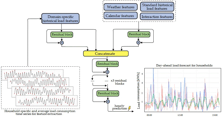
4.3. Proposed Architecture for Household Electrical Energy Consumption Forecast (HousEEC)

In this section, we present our proposed architecture for STLF, which is based on a deep residual neural network. First, we collect daily EE consumption, weather and calendar data. Weather and calendar data are used for extracting contextual features (see Section 4.1.1). From the daily EE consumption data, we extract standard historical load-related features referring to a particular household, or average values for all households in the system. Additionally, we define four time series (see Section 4.1.2) to extract domain-specific historical load features. The values of the extracted contextual and load-related features are then transformed in such a way that their distribution is centered around 0 (has a mean value 0) with a standard deviation of 1. This is done feature-wise, i.e., independently for each feature.

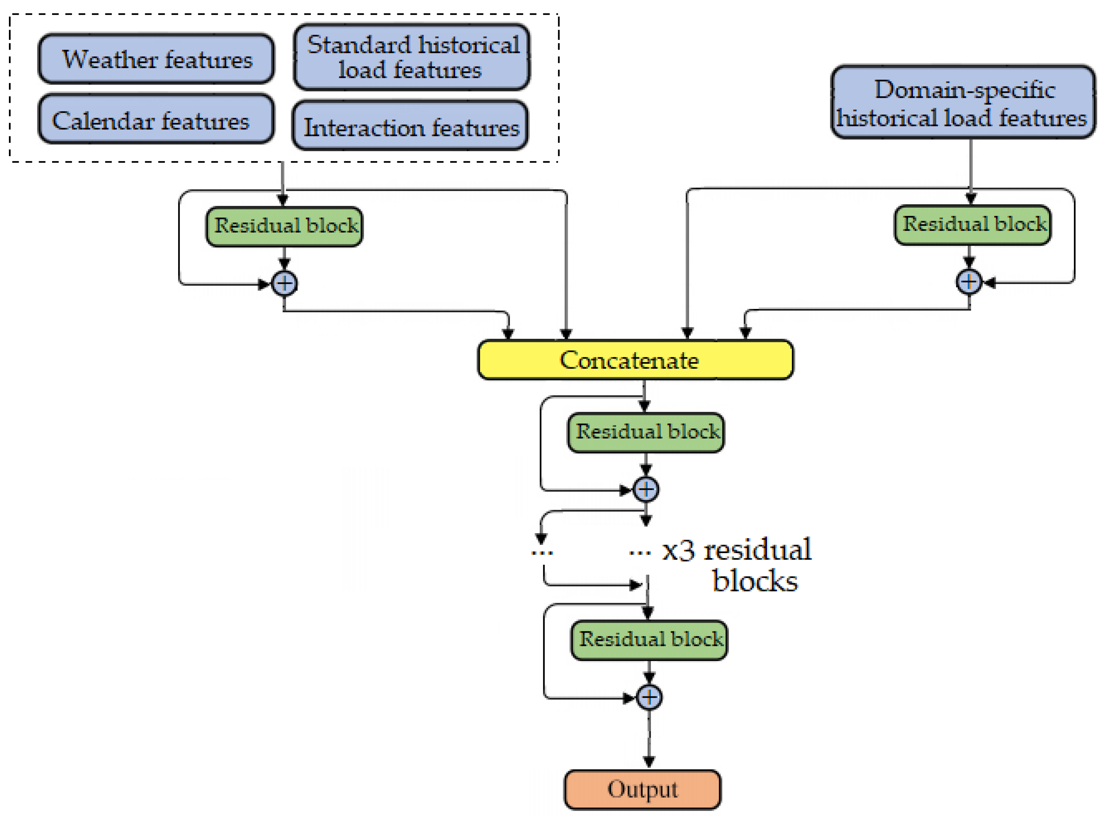
The structure of the DRNN for load forecasting is illustrated in Figure 7. The input features are separated into two groups, and each group is used as input in a separate branch. One branch uses contextual features in combination with the classical historical load features as input, and the other uses only domain-specific features. The left branch starts with a residual block containing 32 neurons in the fully connected layers, while the right branch starts with a residual block containing 64 neurons in the fully connected layers. The use of fully connected layers instead of the original convolutional layers in the residual blocks makes the network more applicable for feature-based input and regression [61]. The output of the first two branches is then concatenated with the raw input features, and as such is fed to a DRNN with five additional residual blocks. Each residual block consists of two fully connected layers, activation function and batch normalization. The fully connected layers in the blocks consist of 64, 32, 16, 16 and 8 neurons, consecutively. All such layers in the residual blocks use ReLu as the activation function. Mathematically, it is defined as f(x) = max(0,x), which makes it suitable for the STLF problem, since the forecasted consumption cannot have negative values. Additionally, we used a dropout rate of 0.1 in order to reduce the chances of overfitting. A total of 6 levels of residual blocks are stacked (1 input level with 2 residual blocks and an additional 5 levels after the concatenation block), forming a 12 layer DRNN.

5. Experimental Setup

5.1. Evaluation Metrics

In order to evaluate and compare the models, several evaluation metrics were used: root-mean-square error (RMSE) [62], mean absolute error (MAE) [63], and R² score [64], which are well-known metrics used to measure performance on regression tasks.

MAE and RMSE are directly interpretable in terms of the used measurement unit (kWh in our case). RMSE is a measure that shows how much the residuals are spread out. Residuals are the difference between actual and predicted values. The definition of RMSE indicates that large errors have higher weight. Since in our regression problem the forecasted values are in a small range, large errors are particularly undesirable. Since we want to penalize large errors more, we focused more on RMSE. MAE shows how close the forecasted values are to actual values. It is calculated as a mean of the absolute values of each prediction error on all instances of the test dataset. R² expresses how well the model replicates the observed outcomes, based on the proportion of total variation of outcomes explained by the model. This metric is positively oriented, and its highest value can be 1. RMSE, MAE and R² scores are calculated as shown in Equation (3)–(5):

$$\mathrm{RMSE}=\sqrt{\frac{1}{n}{{\displaystyle \sum }}_{i=1}^n{\left(y_{predicted}-y_{true}\right)}^2},$$

(3)

$$\mathrm{MAE}=\frac{1}{n}{{\displaystyle \sum }}_{i=1}^n\left|y_{predicted}-y_{true}\right|,$$

(4)

$${\mathrm{R}}^2=1-\frac{{{\displaystyle \sum }}_{i=1}^n{(y_{predicted}-y_{true})}^2}{{{\displaystyle \sum }}_{i=1}^n{\left(y_{true}-y_{average}\right)}^2},$$

(5)

where n is the number of data samples.

5.2. Reference Models

A reference model or benchmark uses simple summary statistics to create predictions. These predictions are used to measure the benchmark performance, and then this result becomes what we compare our ML model results against. For this study, we implemented three baseline models. One model provides the amount of consumed EE by a specific user 24 or 48 h before the hour of prediction. The 24-h-before value is used for prediction of instances in the first interval, midnight to 09:00, and the 48-h-before value is used for prediction of instances in the second interval, 10:00 to 23:00. Another baseline model is the Vanilla multiple regression Benchmark model [19]. This model uses multiple sources of data to predict future load; in particular, polynomials of temperature and their interaction with calendar variables. To enhance the accuracy of STLF, we augmented the Vanilla multiple regression model by adding some lagged load variables, as well as other combinations of variables that enhance the interaction effect. The last benchmark model is seasonal autoregressive integrated moving average (SARIMA) [65].

For more detailed explanation of the reference models, see Appendix C.

6. Experimental Results

To explore the performance of our proposed model in EE consumption forecast, we did a series of experiments. Section 6.1, Section 6.2, Section 6.3, Section 6.4 and Section 6.5 present numerous comparisons of results for disaggregated hourly load forecast, and Section 6.6 presents the efficiency of the proposed method in aggregated load forecast. Section 6.7 presents a general model to overcome the cold start issue.

6.1. Comparison of Forecasting Techniques

To verify the predictive performance of our STLF model, we made comparison with the previously mentioned benchmarks (see Section 5.2), as well as other ML algorithms—linear regression [66], K-nearest neighbors (KNN) [67], decision tree regressor [68], random forest [69], linear SVR [70], gradient boosting [71,72] and xgboost [73] (see Appendix D). We also considered a classic DRNN, comprising five residual blocks, that takes all features together as input for the first residual block.

Table 2. Performance of methods using different feature sets.

Method	Contextual + Standard Historical Load Features			Contextual + Standard Historical Load Features + Domain-Specific Historical Load Features
	RMSE ↓	MAE ↓	R2 ↑	RMSE ↓	MAE ↓	R2 ↑
Linear SVR	1.89	1.27	−0.80	1.91	1.28	−0.84
KNN	1.05	0.59	0.44	1.04	0.59	0.46
Decision tree	1.35	0.80	0.09	0.89	0.47	0.60
Linear regression	0.89	0.52	0.60	0.81	0.48	0.67
Gradient boosting	0.89	0.50	0.60	0.72	0.4	0.74
XGBoost	0.89	0.49	0.60	0.71	0.4	0.74
Random forest	0.96	0.59	0.54	0.64	0.33	0.79
DRNN	0.88	0.49	0.61	0.51	0.28	0.87
Statistical benchmark				1.13	0.60	0.35
SARIMA [65]				1.21	0.75	0.28
Vanilla benchmark [19]				1.00	0.58	0.50
HouseEEC (ours)				0.44	0.23	0.90

shows RMSE, MAE and correlation R² score for each model and the two benchmarks. A comparison of the performance of the models using different sets of features was also conducted. In the first scenario, only contextual features and standard historical load features were used as input. In the second scenario, the proposed domain-specific historical load features were also included. From the results, the benefit of including domain-specific historical load features can be seen. In almost all cases, the proposed domain-specific historical load features significantly improved the model performance. In addition, the results show that our proposed input structure of the DRNN significantly improves the forecasting accuracy. Our proposed model outperformed all other models in both scenarios, achieving RMSE of 0.44 kWh, MAE of 0.23 kWh and R² score of 0.90.

Computation time for execution of models’ training and testing is important for practical implementation in a system, in the case of models retraining with new data and making daily predictions. The training and testing times of the models used in the experiments are shown in

Table 3. Computation time for model training and testing.

Method	Training Time (s)	Testing Time (s)
Linear SVR	2.428	3
KNN	239	10.053
Decision tree	1.849	6
Linear regression	204	3
Gradient boosting	8.383	12
XGBoost	12.232	22
Random forest	12.222	32
DRNN	948	331
HouseEEC	1.016	336

. In all, 2,544,962 instances were used for training and 1,654,499 for testing the models. The deep learning models were trained and tested on NVIDIA Titan X GPU, with 12 GB GDDR5X memory and memory bandwidth of 480 GB/s, while the conventional ML models were trained and tested on AMD Ryzen 7 2700 CPU with 8 cores and maximum clock frequency of 4.1 GHz.

6.2. Error Analysis of Application Scenarios

• Hourly forecast

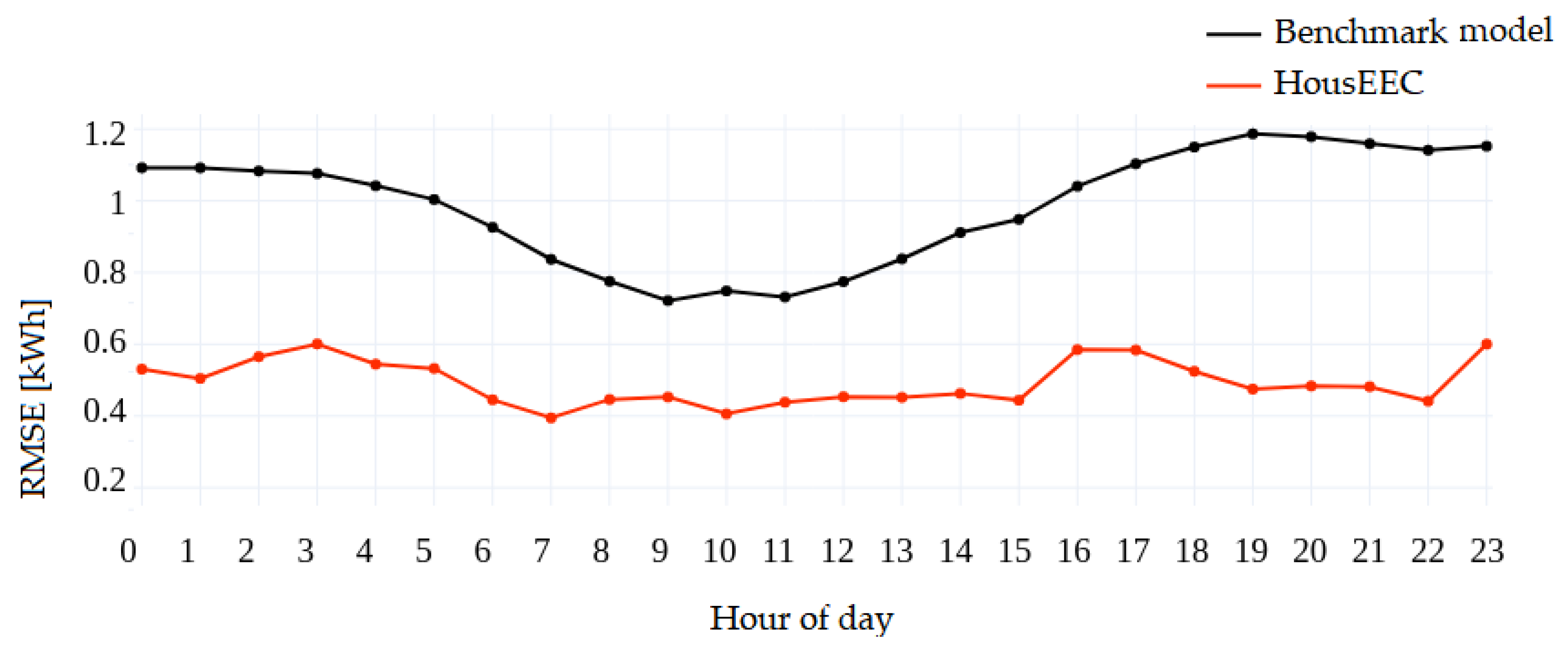
Figure 8 shows the RMSE score for each hour of the day. The results are obtained by averaging the errors for all users for each hour. Larger error can be observed for 03:00, 23:00, and the afternoon hours when most people return from work and perform different activities at home.

However, our model reports quite low error for the morning hours, which is significant because morning hours are related to increased EE consumption, especially on workdays. Overall, there is no significant difference in the reported error for any specific part of the day. Our model significantly outperforms the benchmark model for each hour of the day.

• Weekday forecast

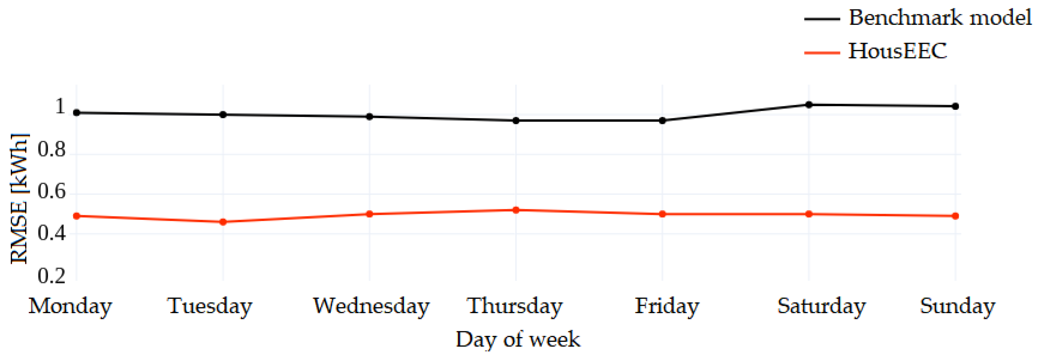
Figure 9 shows the RMSE score for each day of the week. The results are obtained by averaging the errors for all users for each day. The benchmark makes a larger error for weekend days; they are more challenging to forecast due to vacations, trips and irregularities in peoples’ lives. However, our model performs similarly for each day of the week, regardless of the uncertainties that are usually present on weekend days.

• Monthly forecast

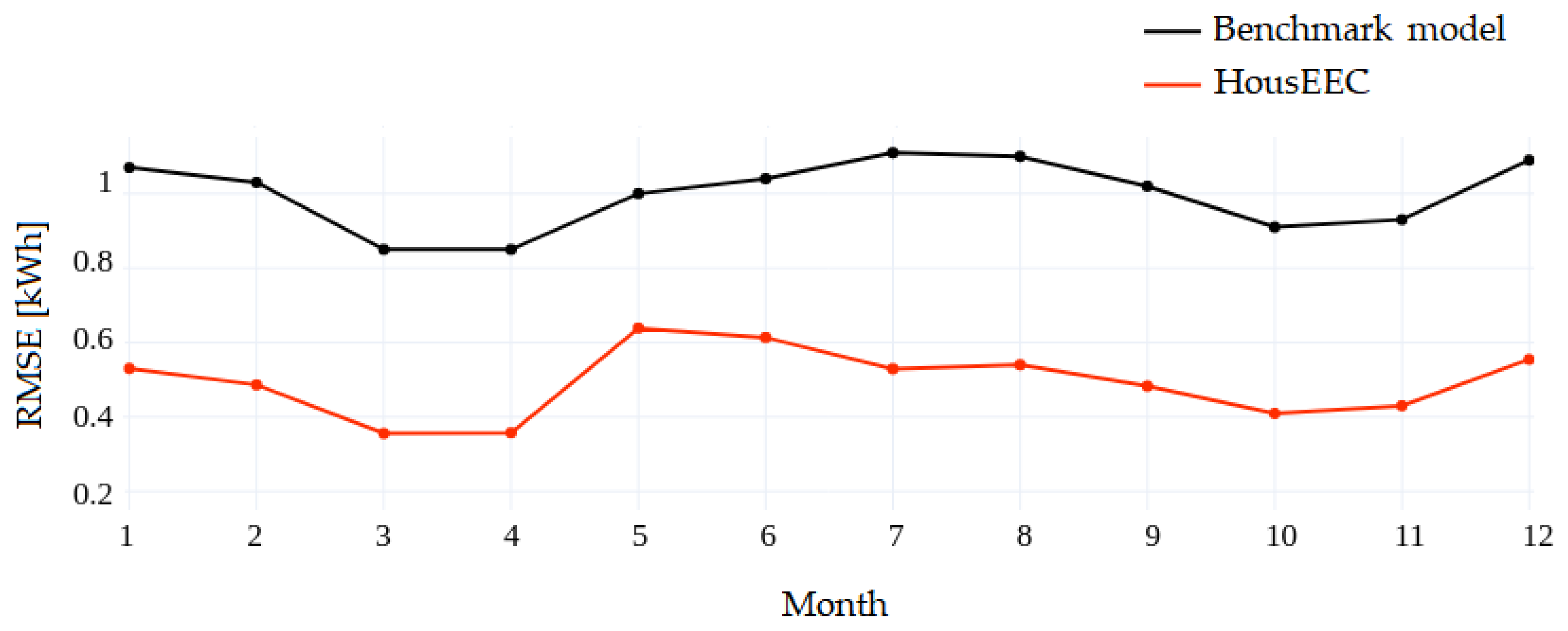
Figure 10 shows the RMSE score for each month of the year. The results are obtained by averaging the errors for all users for each month. Both the benchmark and our proposed method follow a similar trend in terms of the prediction error; the RMSE score is lowest for the spring months when there is no need for heating or cooling. The largest error made by our model can be observed for May, when the cooling season starts. However, after some time, the increased trend of EE consumption is incorporated into the extracted features, so the prediction errors start decreasing. This is a very important characteristic of our model, since the rest of the summer months are also characterized by increased EE consumption. This is certainly not the case with the benchmark model, which reports the largest error when EE consumption is at its peak.

6.3. Comparison with Other Deep Learning Approaches that Use only Time Series

We additionally made performance comparisons between our method and the most recent DL architectures relevant to load forecasting, described in [74]. The authors present seven architectures designed for 24 h prediction and evaluate them using the individual household electric power consumption (IHEPC) [75] dataset, which contains 47 months of EE consumption data of single households. Based on their results, we chose the five best architectures and evaluated them using the Pecan Street dataset with classical feedforward neural network (FFNN), deep residual neural network (DRNN), temporal convolutional network (TCN), long short-term memory (LSTM) and gated recurrent unit (GRU). This DRNN uses different residual blocks compared to the one in our proposed model. All mentioned networks are described in detail in the paper. For this evaluation, we used seven week-long time series as input for the networks, two related to the historical load and five related to weather data. The first time series is actual EE consumption by a specific household in the past week, and the second is average load consumption by all households in the past week. The weather-related time series are temperature, humidity, apparent temperature, wind speed and precipitation. The Pecan Street dataset contains weather and load measurements for each hour, resulting in 168-hourly-measurements long input and 24-hourly-measurements long output for the networks. Since the results in the paper showed that including calendar information improves prediction accuracy, we additionally included the following information: hour of the day, day of the week, month and work-/non-workday. For training, we used the multiple input–multiple output (MIMO) strategy, meaning that a single predictor is trained to forecast a whole 24 values-long output sequence in a single shot.

Table 4. Performance of end-to-end deep learning (DL) approaches.

Method	RMSE	MAE	R2
FNN	1.05	0.70	0.47
DFNN	0.84	0.55	0.53
TCN	0.78	0.50	0.59
LSTM	0.81	0.54	0.54
GRU	0.80	0.54	0.54
HousEEC	0.44	0.23	0.90

shows the results: HousEEC shows better results in terms of RMSE, MAE and R² compared to end-to-end DL-based methods for load forecasting on the household level. The main conclusion that can be drawn from these results is that the time-series consisting of 168 historical load values does not contain enough information for proper training of DL end-to-end architectures. However, one-week historical load appears to be enough for proper training of the feature-based DRNN, especially when it is trained with extensive feature sets consisting of the domain-specific features which give new insights into the load time-series dynamics.

6.4. State-of-the-Art STLF on Household Level

The STLF field lacks a unified comparison between conducted studies. There are many studies in this field that address different segments related to load forecasting, and most of them are not directly comparable. Nevertheless, we believe that a summary of the results achieved with state-of-the-art methods might be informative and useful for new studies in a few ways. Authors can select the most commonly used dataset for their work in order to produce comparable results, and it can help researchers to avoid selecting nonrepresentative data for evaluation of their methods. In this section, selected studies relevant to STLF on the household level are presented. The two criteria for study selection were the forecasting horizon (up to 24 h) and the evaluation metric (RMSE). In order to include more relevant studies, we additionally considered studies reporting normalized root mean squared error (NRMSE), calculated as shown in Equation (6):

$$\mathrm{NRMSE}= \frac{\sqrt{\frac{1}{n}{{\displaystyle \sum }}_{i=1}^n{\left(y_{predicted}-y_{true}\right)}^2}}{\frac{1}{n}{{\displaystyle \sum }}_{i=1}^n{y}_{true}}.$$

(6)

We ended up with 12 relevant studies, including ours.

Table 5. Summary of state-of-the-art STLF studies.

Authors	Forecasting Horizon	Number of Households	Duration of Evaluation	RMSE	NRMSE
Shi et al. [40]	1 h	920	1 month	0.45	–
Lusis et al. [76]	30 min	27	28 days	0.52	–
Muralitharan et al. [77]	24 h	–	–	0.62	–
Gasparin et al. [74]	24 h	1	12 months	0.75	–
Yildiz et al. [78]	24 h	14	–	0.80	–
Ali et al. [79]	1 h	34	6 months	0.80	–
Ganz et al. [80]	24 h	74	2 months	0.85	–
Gerossier et al. [81]	24 h	226	2 months	–	0.43
Vos et al. [82]	24 h	200	6 months	–	0.53
Wijaya et al. [83]	24 h	782	6 months	–	0.61
Humeau et al. [50]	24 h	782	6 months	–	0.80
HousEEC	24 h	297	12 months	0.44	0.34

presents a summary of the studies in terms of forecasting horizon, number of households used for evaluation, duration of the test data, and results achieved in terms of RMSE (NRMSE). One parameter that should be considered in this comparison is the size of the data used for evaluation. EE consumption is highly affected by the weather; a lot of electricity is used for cooling in summer and heating in winter. This leads to the conclusion that studies that use shorter periods for their evaluation might present unreliable results without checking model performance in different seasons. Only one of the selected studies evaluated their methods using data collected in a period of 12 months. In order to show how robust the proposed methods are, more households are needed for evaluation. This is because there are different types of users, such as elderly people who spend most of the time at home, people who go to work, students who have a dynamic lifestyle, etc. Only four studies considered datasets with fewer than 100 households.

For our work, we addressed the previously mentioned challenges; our model provides forecasting one day ahead, and the results are evaluated on 297 households over a period of one year. We believe that our results are very promising, considering that they show great performance of the model for a large number of households evaluated for a period of 12 months.

6.5. Analysis of Different Lengths of Training Set

Over time, new households with different EE consumption patterns can appear in the forecasting system. Therefore, it is a common practice for forecasting models to be trained with new data after a certain time. This section presents the HousEEC model’s performance for three subsets of the initial test set, when additional data is used for training. For comparison, we used the final HousEEC model (trained with 27 months) to predict the EE consumption of the three new test subsets.

Table 6. Performance of models with different train-test splits.

	Train-Test Splits (M—Months).
	27 M vs. 9 M	30 M vs. 9 M	27 M vs. 6 M	33 M vs. 6 M	27 M vs. 3 M	36 M vs. 3 M
RMSE	0.43	0.46	0.47	0.48	0.45	0.45
MAE	0.28	0.27	0.27	0.28	0.24	0.25
R2	0.92	0.9	0.9	0.9	0.9	0.92

shows the RMSE, MAE and R² scores for different train-test splits.

Even though it is expected that constant inclusion of new data expands the knowledge of the existing model, the results from this analysis showed that there was no significant benefit of it when there were no changes in the dataset in terms of new households.

6.6. Aggregated Consumption Forecasting

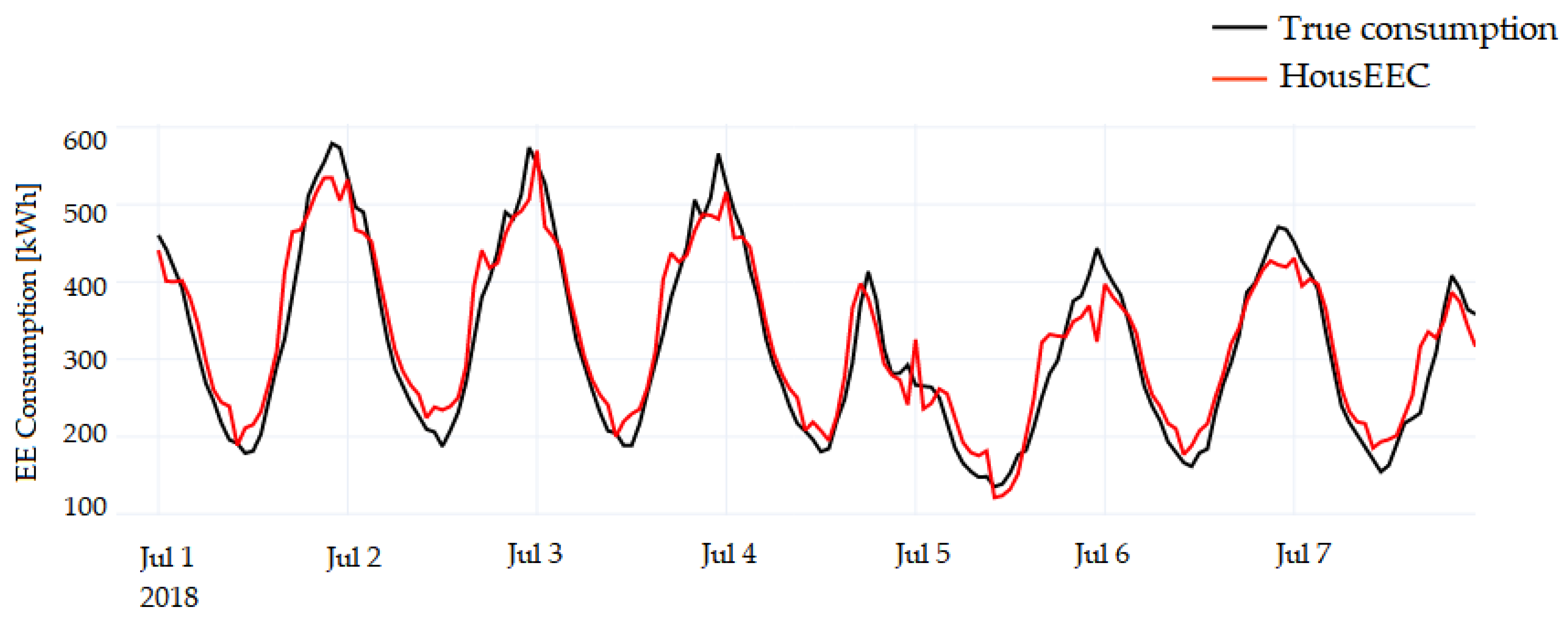
Forecasting of aggregated load can be implemented by the standard strategy of direct forecast of the aggregated load, or by aggregating the forecasts for individual households. In Figure 11, we observe the curve of aggregated forecasts for all households and compare it to the actual aggregated load curve. The observed period is the first week of July. It is one of the hottest months in the year, characterized with increased EE consumption due to air-conditioning (Figure 3). Since the peak EE consumption is the most challenging to forecast, we more closely observed the model’s performance for a whole week in July—the month during which the EE consumption is the highest in our dataset. It is obvious that the forecast successfully follows the trend of actual consumption, even for July 5, when a significant drop of EE consumption is noted, which is not typical for the time period observed.

Finally, we calculated total consumption of all households and total error for hourly and daily analysis. The hourly analysis showed that, on average, the aggregated EE consumption of the households is 263 kWh. Our model makes 8% error on average per hour forecast (22 kWh); the Vanilla multiple regression benchmark makes 12% error (32 kWh). The daily analysis showed that, on average, the aggregated EE consumption of all households is 6140 kWh. Our model makes 2% error on average per day forecast (131 kWh); the baseline makes 6% error (360 kWh).

6.7. Cold Start Issue

In order to predict next-day EE consumption of a new household in the system, the HousEEC model requires the household’s historical EE consumption of the previous week. This means that it suffers from a one-week cold start, which is a technical limitation of the model. To overcome this limitation, we trained an additional general model that does not use household-specific standard historical load features and domain-specific historical load features that are extracted from the third type of time-series (see Figure 5). This model will to serve as a model for prediction of household EE consumption for only the first week. We used the same HousEEC architecture, and the only difference was the number of input features. The performance of this model on the same test set used in the previous experiments can be seen in

Table 7. Comparison of performance of general and HousEEC models.

Method	RMSE	MAE	R2
General model	0.50	0.26	0.87
HousEEC	0.44	0.23	0.90

. As expected, this general model provided less precise results compared to the final HousEEC model. However, we consider these results as acceptable, given that this general model would be used for only a short period of time in an actual implementation of the system. The presented results are also additional evidence of the significance of domain-specific historical load features for a particular household.

7. HouseEEC System Prototype

This section presents the practical implementation of the HousEEC system and deployment of the ML model in a prototype web application. The system enables end users to quickly and easily access a service that allows different analyses. One of the most important features of this system is that it can be easily implemented in larger systems that have different monitoring devices for electricity consumption in households. The only prerequisite for implementing such a system for analyzing and forecasting electricity consumption is access to the measured values of household EE consumption. The system contains three main modules:

• Graphical user interface (GUI), through which forecasts of EE consumption can be accessed.
• Back end, which provides the functionality that is served to users through the graphical interface. This section is also responsible for communication with the database, deployment and launch of the forecast module, and similar functions. It also provides application program interfaces (APIs) for interconnection with the ML module and the GUI.
• ML module, which is responsible for deployment of the ML model and its practical use. It contains all the steps required for an ML pipeline: preprocessing data and dealing with missing data; extracting features; and predicting with the ML model. For the implementation, we used libraries including Pandas, Sklearn, NumPy, Tsfresh, SciPy, Keras and Tensorflow.

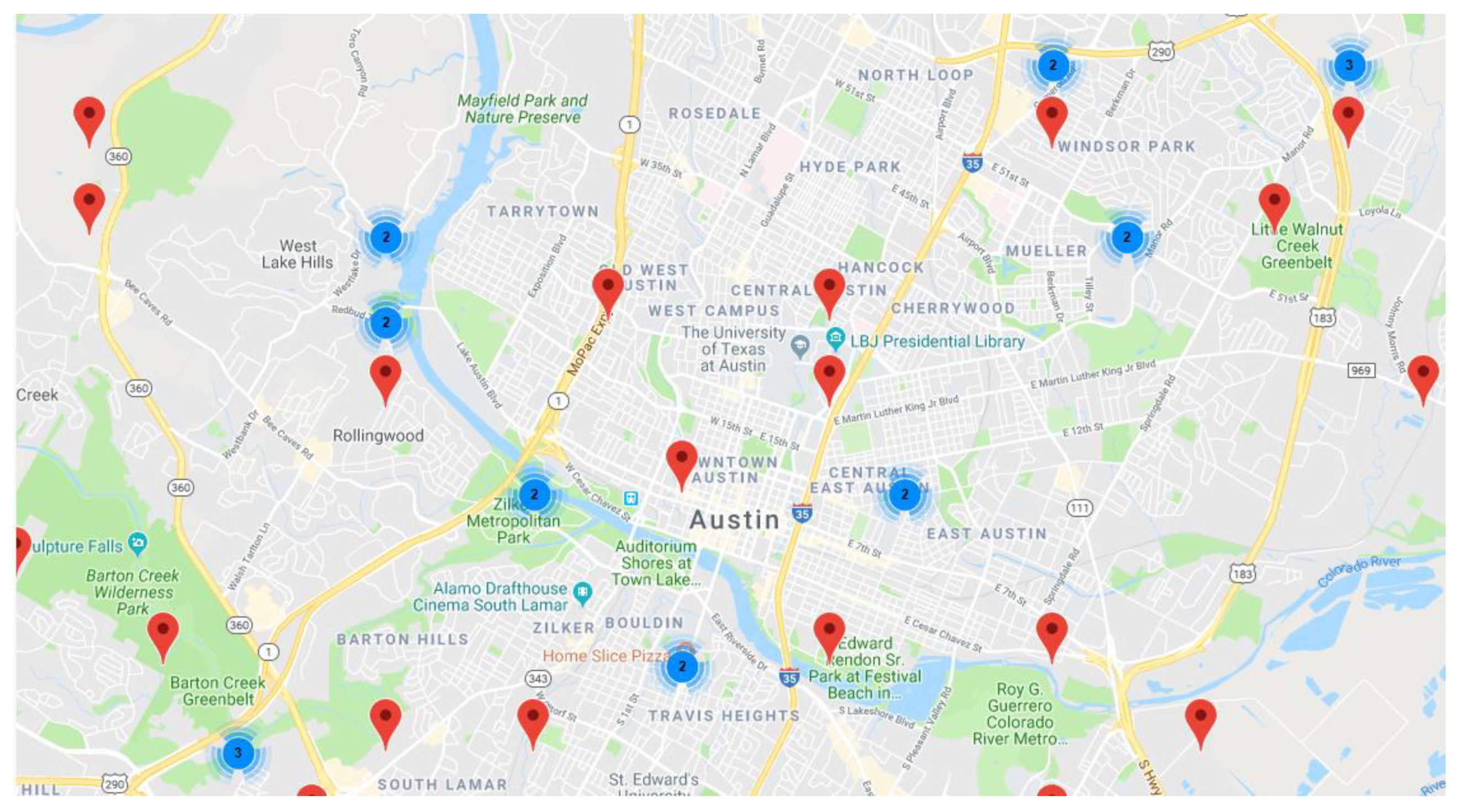
A visualization of the system and its households is shown in Figure 12. For better visualization, multiple households that are very close geographically are presented as a group (blue circles on the map). Note that this is a simulation, and the geographic locations are for illustration purposes only; the dataset does not contain location information about the households. Next, the application provides access to a table of measured EE consumption of all households for the last 24 h. In addition, there is an option to search for a specific household, which can provide insight into its individual time series of EE consumption. This table also enables easy control of the accuracy of household measuring devices: whether they show values or whether there are erroneous values in the metered data (negative values for consumed electricity or values outside the expected range). If unexpected data are spotted in the table, they can be deleted from the database, preventing them from affecting prediction by the ML model in the following days.

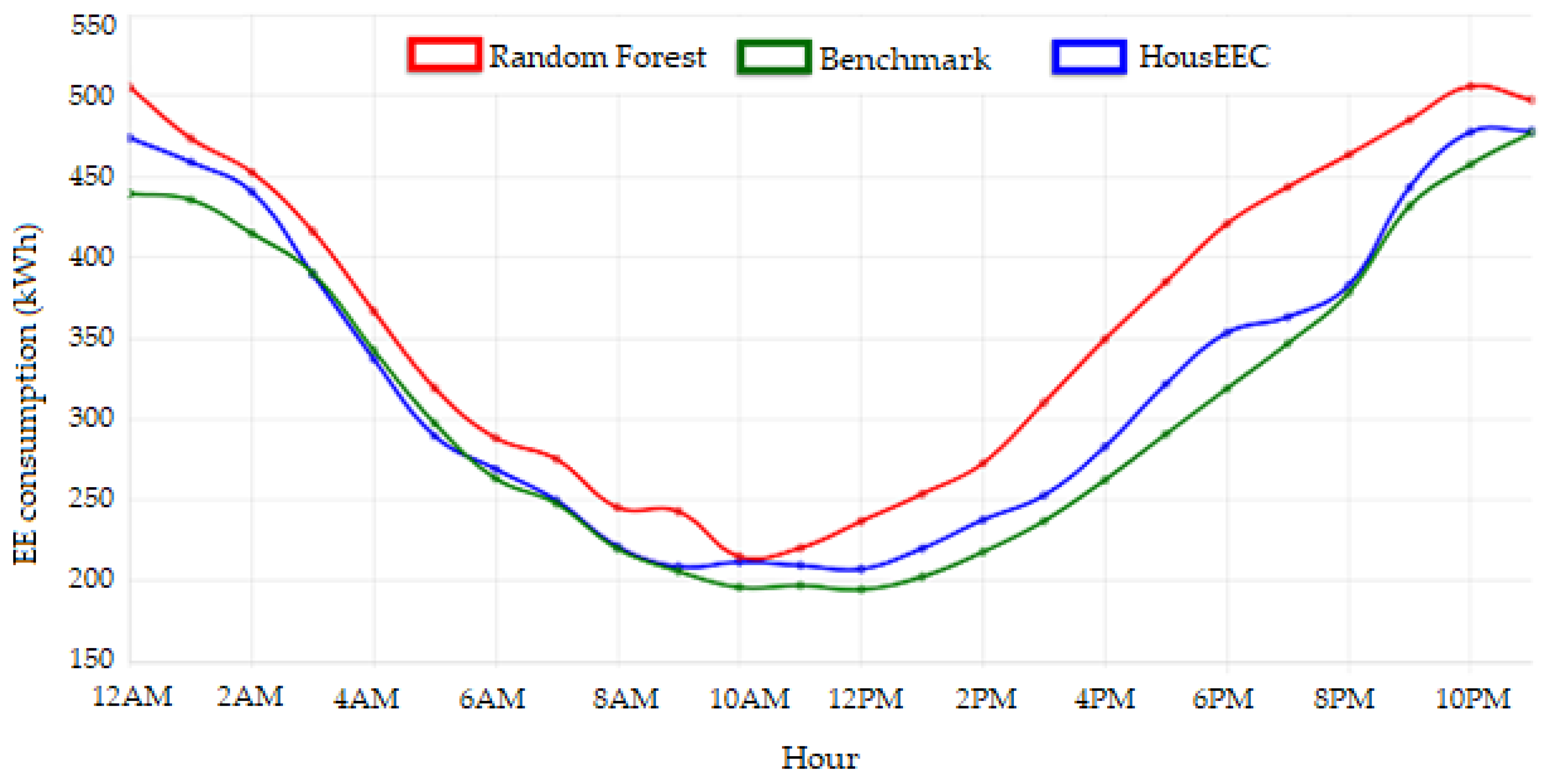
The next service of the system represents daily predictions of EE consumption for each hour of the next day. These forecasts are obtained by executing the ML model at 10:00 every day. This allows sufficient time for planning the actions of the day-ahead electricity market, which, as mentioned before, closes at 12:00. Although forecasts are obtained at the household level, they are presented at the aggregated level for all households. Figure 13 shows three lines, representing predicted electricity consumption achieved by the three chosen models: random forest, benchmark and our final HousEEC.

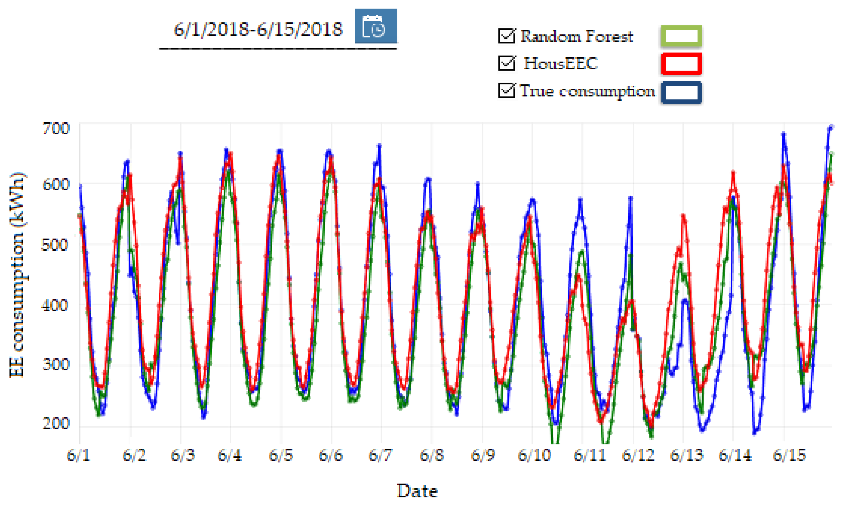
The final service offered by the system is the performance analysis of the ML models (Figure 14). With this service, users can load predictions for the past period and compare them to actual consumption values. First, the user selects the interval of interest and the models. Then the system outputs the predictions and true consumption. For example, Figure 14 shows predictions of the random forest and HousEEC models and the true consumption for the randomly selected period from 1–15 June 2018. The user can visually inspect the model errors.

When using real-time data collection devices, it is inevitable that some amount of data gets lost due to different circumstances (sensor fault, communication error, environmental disturbance, etc.). In this context, the use of techniques that deal with missing data is a crucial part of the implementation of a forecasting system. To guarantee that our forecasting system would work smoothly, we considered two cases of missing data and appropriate techniques to handle it. The first case is missing values of EE consumption for one hour for a particular household. For this case, we implemented linear interpolation, a mathematical method that adjusts a function to the existing data and uses it to extrapolate the missing data. The second case is when sensor readings are missing for two or more consecutive hours for a particular household. In this case, the missing values are replaced with the forecasted values for those hours by the HousEEC model (or the general model, if the missing values occur in the first week of the data collection process for the household; see Section 6.7).

8. Conclusions

The paper presents the HousEEC system, which provides day-ahead household EE consumption forecasting using a deep residual neural network. The experimental evaluation was performed on one of the richest datasets for household EE consumption, the Pecan Street dataset. The DL approach combines multiple sources of information by extracting features from (i) contextual data (e.g., weather, calendar), and (ii) the historical load of the particular household and all households present in the dataset. Additionally, we computed novel domain-specific time-series features that allow the system to better model the pattern of household energy consumption. Their contribution to reducing the error is shown in Table 2. Finally, we assessed performance by comparing the results achieved with our model with those of seven other ML algorithms, five DL and two benchmarks widely used in this area.

The experimental results show that in all cases, our model outperformed every other algorithm and approach, achieving RMSE of 0.44 kWh, MAE of 0.23 kWh and R² score of 0.90. The analysis shows the great potential of including our domain-specific historical load features in improved load forecasting. The hourly analysis showed that all customers used 263 kWh per hour on average. Our model makes 8% error on average per hour forecast (22 kWh), which is 4 percentage points better than the benchmark model results. The daily analysis showed that all households used 6140 kWh per day on average; our model makes 2% error on average per day forecast (131 kWh) and the benchmark model makes 6% (360 kWh). The comparison between end-to-end DL architectures and our proposed DL feature-based architecture showed that our method performs better, achieving significantly lower RMSE compared to the best performing end-to-end DL architecture, the temporal convolutional network. We believe that the main reason for this improvement is the domain-specific features, which give the algorithms the most relevant information derived from the raw data for future load forecasting. According to the analysis of similar studies for STLF for households, we can say that our achieved results are very promising compared to the state-of-the-art approaches. We also believe that our study shows reliable results because the method was tested on a significantly large number of households over 12 months using a 24 h forecasting horizon.

The proposed method, which predicts EE consumption on an individual household level, offers great commercial potential because it is scalable and not dependent on the current number of households in the system. In addition, predicting individual forecasts enables their aggregation, which yields better forecasting for the aggregation level compared to the conventional strategy of direct forecast of the aggregated load [25,84]. Our method also has significant value because it is not dependent on the number of households included in the system. Implementation of the system does not suffer from cold start; we addressed the cold start problem by introducing a new general model that does not use household-specific historical load features. This model is intended to provide predictions for each new household that appears in the system for the first week, until the required data for the HousEEC model is collected. Another important detail that we considered in the system implementation is the occurrence of missing data. We tackled this by using two techniques, interpolation and the use of forecasted values to fill the missing data in the EE consumption of a particular household.

We expect that the final model could perform well on other datasets which contain EE consumption data for households with similar economic status, located in places with similar weather conditions. It was trained with data from a large number of households, which make it more general, robust and able to adapt to many different EE consumption patterns. Additionally, if the HousEEC architecture is used for model re-training with new data, we expect it to show equally good performance, since it incorporates data from multiple relevant sources that affect the EE consumption of households. However, further investigation of the model’s performance on other datasets is considered for future work.

Another improvement would be to introduce additional features, such as EE price, number of household members, age of users, daily schedule of users (working hours), size of household, and means of heating and cooling. We believe that these attributes would improve the accuracy; however, this requires additional private information about households, which might not be easy to obtain.

Finally, we plan to introduce the clustering of households, because there are different trends and patterns for each household in the dataset and there are large variations in the electricity consumption patterns at the household level. A clustering algorithm would group similar households into clusters and, in a way, define household profiles. This way, there will be several prediction models for different clusters of households. We believe this can increase the forecasting performance, because there are several types of users (active users who regularly go to work, older users who spend the biggest part of the day at home, etc.), and it is more difficult for the model to acquire a knowledge about the EE consumption characteristics of different users.