A Model Predictive Control Strategy for Distribution Grids: Voltage and Frequency Regulation for Islanded Mode Operation

Abstract

In the last few years, one of the most important challenges of power technologies has been the integration of traditional energy production systems and distributed energy resources. Large-scale photovoltaic systems and wind farms may decrease the quality of the electrical grid service, mainly due to voltage and frequency peaks and fluctuations. Besides, new functionalities, such as the operation in islanded mode of some portions of the medium-voltage grid, are more and more required. In this respect, a model predictive control for voltage and frequency regulation in interconnected local distribution systems is presented. In the proposed model, each local system represents a collection of intelligent buildings and microgrids with a large capacity in active and reactive power regulation. The related model formalization includes a linear approximation of the power flow equations, based on stochastic variables related to the electrical load and to the production from renewable sources. A model predictive control problem is formalized, and a closed-loop linear control law has been obtained. In the results section, the proposed approach has been tested on the Institute of Electrical and Electronics Engineers(IEEE) 5 bus system, considering multiple loads and renewable sources variations on each local system.

1. Introduction

The increase of intermittent renewable energy sources (RES) has created instability issues, requiring new controllers for modern smart microgrids [1,2,3]. Actually, RES may cause voltage/frequency peaks and fluctuations that negatively affect the quality of the electrical grid service. On the other hand, RES represents an important alternative to reduce global fossil fuel consumption. The need for new control strategies is also motivated by the increase of distributed small generators that cause millions of new producers potentially involved in the energy market. In such a scenario, in the balancing market, new actors, such as aggregators [4], are present and new functionalities are more and more required. For example, in order to preserve the electrical grid from faults and emergency situations, it may be necessary to reduce the power demand and to operate some portions of the medium-voltage grid in islanded mode. These new set-ups require new fast controllers, which can take into account voltage and frequency models.

In addition, the grid operators, i.e., the transmission system operator (TSO) and distribution system operator (DSO), are forced to deeply change their roles. As an example, the DSO must become active in its activities as a grid manager [5]. The DSO, in particular, is responsible for the normal operation of the distribution grid and its subsystems (i.e., managing power quality and energy losses). Among others, the new roles for the DSO are: operational security management, dynamic voltage and frequency control, outages response, performing restoration actions, and market operations. In this framework, it becomes hard to define an effective optimal control, which derives from the structure of the power grid, and, specifically, from the presence of several issues: renewable and traditional power production, bidirectional power flows, and stochastic modelling issues (due to uncertainties in forecasting power generated from renewable resources). The main challenge is to define and to solve control problems embedding prediction models for the regulation of frequency, voltage, and active and reactive power flows. Indeed, the complete power flow equations are nonlinear and nonconvex [6]. Therefore, optimization problems can hardly apply them to compute the control in real time. On the other hand, there is the need to represent in detail the physical system to provide reliable control strategies [7].

This work focuses on the optimal control of interconnected local systems in a distribution grid. A local system can represent a group of renewable generators, passive and active loads, or microgrids with a large capacity for active and reactive power regulation. The proposed approach can be used:

• To reduce frequency oscillations and to improve inertia response due to a sudden change in the grid (i.e., a variation on a renewable power plant production), and
• To manage a portion of the distribution grid that is operated in islanded mode because of demand response programs and/or emergency requirements.

In fact, an increase in the RES penetration can decrease the number of generation units that provide reserve power for primary and secondary control. So, the frequency deviation increases [8]. New equations for inverters’ control to regulate frequency and voltage are required when a change in the grid occurs (e.g., a loss of load).

The modelling approach proposed in this paper is based on the concept of virtual inertia [9,10,11]. An electrical model is defined, including voltage (magnitude and phase), frequency, active and reactive power, and stochastic components. So, the definition of an optimal control problem for frequency and voltage regulation in multi-local systems is introduced. The aim is to define a closed-loop controller for the mitigation of frequency and voltage variations.

The paper is organized as follows. Section 2 reports the state-of-the-art and discusses the innovation of the proposed work. In Section 3 and Section 4, the system and the optimal control problem are formalized. Finally, the application to a case study is described in Section 5, while conclusions and future developments are reported in Section 6. The Appendix A reports proofs related to demonstrations not included in the text for sake of readability.

2. Literature Review

Nowadays, the control of interconnected local distribution systems is a challenging problem. In this respect, several papers focus on the definition and solution of optimization and control problems. A detailed survey [12] on multi-microgrids systems has been recently published, where operational management and control are quoted as challenging problems to be faced. Zheng et al. [13] propose a distributed model predictive control (MPC) approach using discrete-time Laguerre functions for load frequency control in multi-area interconnected power systems, in order to overcome the problems of computational burden and online optimization. The advantage of an MPC approach is that it allows for implementing a multivariable controller that controls the outputs simultaneously by taking into account all the interactions among system variables. Another strength of MPC (not used in our work, where a closed fast feedback is adopted) is that it can handle constraints. Khooban and Niknam [14] propose a heuristic algorithm and a fuzzy logic approach to tune parameters of classical proportional integral (PI) controllers for multi-area load frequency control. However, electrical models are not detailed. In the literature of microgrids, there are several interesting approaches based on MPC but related to the single microgrid, and thus not interconnected with other local systems. In Reference [15], a novel fractional-order model predictive control method is proposed to achieve the optimal frequency control of an islanded microgrid by introducing a fractional order integral cost function into the MPC approach. As in the present work, frequency regulation is attained, even if hereinafter we propose a more detailed system model, where active and reactive powers are present and voltage is regulated.

In Reference [16], a feedback linearization is applied to design a predictive controller for the secondary control of the voltage and frequency in an islanded microgrid. The goal is to improve the performance of a closed-loop nonlinear system. The control scheme is fully distributed, and necessary and sufficient conditions for convergence and stability of the whole system are described. As a similar approach, we model both active and reactive power, but providing a control strategy for the whole optimization problem that can be used under a MPC scheme. In Reference [17], a MPC-based controller uses a simplified voltage prediction model to predict the voltage behavior in an islanded microgrid. Apart from the fact that we consider multiple microgrids, in our model, we use a more detailed electrical model and we derive an optimal control law. The same considerations can be done in comparison with References [18,19].

The approach considered in the present paper gives a strong emphasis on the model of the electrical grid. Specifically, the approach is based on the concept of virtual inertia [20,21]. The problem of virtual inertia control is mainly felt in microgrids and grids where RES are present, as it is necessary to cope with small inertia and uncertainties. In Reference [22], the authors propose an approach to increase the inertia of the photovoltaic (PV) system through inertia emulation, which can be obtained by controlling the charging/discharging of the DC-link capacitor and adjusting the PV generation. Wu et al. [23] consider an islanded microgrid with renewables and storage systems, in which virtual inertia allows power curtailment of RES units and demand response (loads’ shifting). In fact, these approaches are also useful for islanded microgrids, and several works are present in the recent literature for frequency and voltage regulation, and for stability [24,25,26,27,28].

In Reference [24], the authors assess that droop control methods are not suitable for renewable energy-based microgrids due to their limited capability for power delivery. They propose a supercapacitor-based DC-link voltage stabilizer and a battery energy storage system-based frequency stabilizer. In particular, as in Reference [25], a fuzzy-based controller is proposed. In Reference [26], the authors highlight the drawbacks of PI controller gains and propose the Grasshopper Optimization Algorithm to optimize the PI controller parameters.

An additional critical issue is represented by the demand of electric vehicles in a smart grid. To face such problem, in Reference [27], distributed controllers are proposed. Other papers [28] focus on improvements of droop controllers and on new approaches for the optimal dispatch in hierarchical microgrids [25]. Specifically, two control modes are considered for the generation units: a voltage control mode, with an active droop control loop, and a power control mode, which allows setting the output power in advance. Some recent works that study virtual inertia are References [29,30,31,32,33]. In Reference [29], the authors study a novel control scheme for virtual inertia converters to operate in unbalanced settings, operating test on real hardware. In Reference [30], an adaptive controller method for a PV-based virtual inertia system is discussed. The approach is studied in the case of the small-signal stability and low-frequency oscillation, which are characteristics of the PV generators. In Reference [31], the authors aim at improving the inertia of a microgrid by reducing the time delay of the communication system to overcome frequency oscillations, finding a compromise with the increase of operational costs.

In Reference [32], the authors propose an approach to find the proper value of inertia constant, together with the frequency droop coefficient of DERs (distributed energy resources) and tuning load frequency controllers’ parameters to improve the frequency stability. A multi-objective decision problem is formulated in which the following goals are considered: minimizing the maximum frequency deviation while promptly bringing the frequency back to the desirable region, and minimizing a higher inertia constant that results in a higher cost of energy storages. With a significant difference, here, we propose an optimal control problem to minimize frequency and voltage deviations for multiple microgrids and the optimization problem is analytically solved taking into account both active and reactive power.

In Reference [33], virtual inertia in islanded microgrids is studied. An H-infinite (H∞) robust control approach to the virtual inertial control loop is implemented, taking into account the high penetration of renewables, thus enhancing the robust performance and the stability of the microgrid during contingencies. In the present paper, we propose a control law to minimize frequency and voltage deviations taking into account both active and reactive power under an MPC scheme.

Hereinafter, the electrical grid connecting different local systems is modelled. This paper aims at studying the regulation of voltage and frequency within local systems interconnected through a distribution network. Since these systems have a strong renewable, uncontrolled, and intermittent component, they intrinsically represent a disturbance that, if not controlled, may cause a decrease in the system performance and quality. It is worthwhile to observe that the problem faced is not to be confused with the classic problem of inter-area oscillations between systems connected by a high-voltage grid.

In this work, an MPC approach is proposed, taking into account uncertainties, and deriving an optimal solution that can be used in closed-loop and in real time. In the literature of power systems, similar control approaches can be found [34,35]. Delfino et al. [36] propose a multilevel architecture for interconnected microgrids in which the DC power flow equations are used at a higher level, an analytical solution emulates each microgrid, and the AC power flow equations are used at the lower level. Minciardi and Robba [37] formalize a decision model in which a stochastic optimal control problem is defined and solved. An optimal control strategy can be also found in Reference [38]. The authors consider the problem of load-frequency control in a multi-area power system proposing a hierarchical optimal robust controller. They decompose the overall problem in subsystems, solve the lower level through a control strategy, and finally, iteratively coordinate local systems. However, a detailed representation of the electrical network is not present. Annaswamy and Kiani, in Reference [39], include a discrete-time decentralized linear quadratic regulator (LQR) controller in a transactive architecture for hierarchical smart grids. In the present paper, with respect to References [34,35], a detailed representation of the electrical network is included in order to regulate voltage, and control active and reactive power. With respect to References [36,37], the decision problem has been solved analytically. In addition, References [34,35,36,37,38,39] do not consider frequency variations and equivalent inertia. Other optimal control strategies for the smart grid are present in the literature [40,41] but not in the area of interconnected local systems.

In summary, the main contributions of the proposed paper are:

• The statement of the frequency and voltage control problem of distribution grids in islanded mode expressed as an MPC of an affine system affected by additive noise.
• The inclusion of models for the control of frequency, voltage, and active and reactive power in distribution grids.
• The derivation of an analytical solution for the stochastic MPC problem based on a two-stage decomposition.
• An optimal control strategy for the inter-local systems variation problem that can be used either for frequency and voltage regulation or the operation in the islanded mode of portions of the distribution grid for demand response purposes.

3. The System Model and the Optimization Problem

Consider a distribution power grid (Figure 1) modeled as an undirected graph G = (A, L), where the set of nodes $A=\left\{1,\dots ,N\right\}$ characterizes the set of local systems and $L=\left\{1,\dots ,b\right\}$ is the set of links that connect the nodes. Specifically, each local system is interfaced with the distribution grid by a power converter which can perform a virtual inertia control (allowing the inverter to behave as a fictitious synchronous generator) with equivalent inertia time constant $H_i$($i\in A$) and damping factor $K{D}_i$($i\in A$). The set of arcs, L, represents the set of lines that connect the local systems—each line has a proper impedance $Z_{i,j}=R_{i,j}+j{X}_{i,j} \left(i,j\in A\right)$, with $R_{i,j}\hspace{0.17em}\hspace{0.17em}\left(i,j\in A\right)$ being the line resistance and $X_{i,j}\left(\hspace{0.17em}\hspace{0.17em}i,j\in A\right)$ being the line inductance. All local systems are composed of different devices: distributed controllable resources with high regulation capacity (denoted by G), reactive power-regulating sources (denoted by NG), renewable non-controllable resources (denoted by RES), and passive loads (denoted by L). Each local system can be modeled as an equivalent synchronous generator with equivalent inertia to consider its contribution to the frequency regulation of the whole grid.

In the following paragraphs, the state and the control variables are defined, and the optimization problem is formalized. All the quantities (but the phases) and the equations are expressed at discrete time per unit (p.u.) values. As suggested by the literature, this method offers computational simplicity by eliminating units and expressing system quantities as dimensionless ratios.

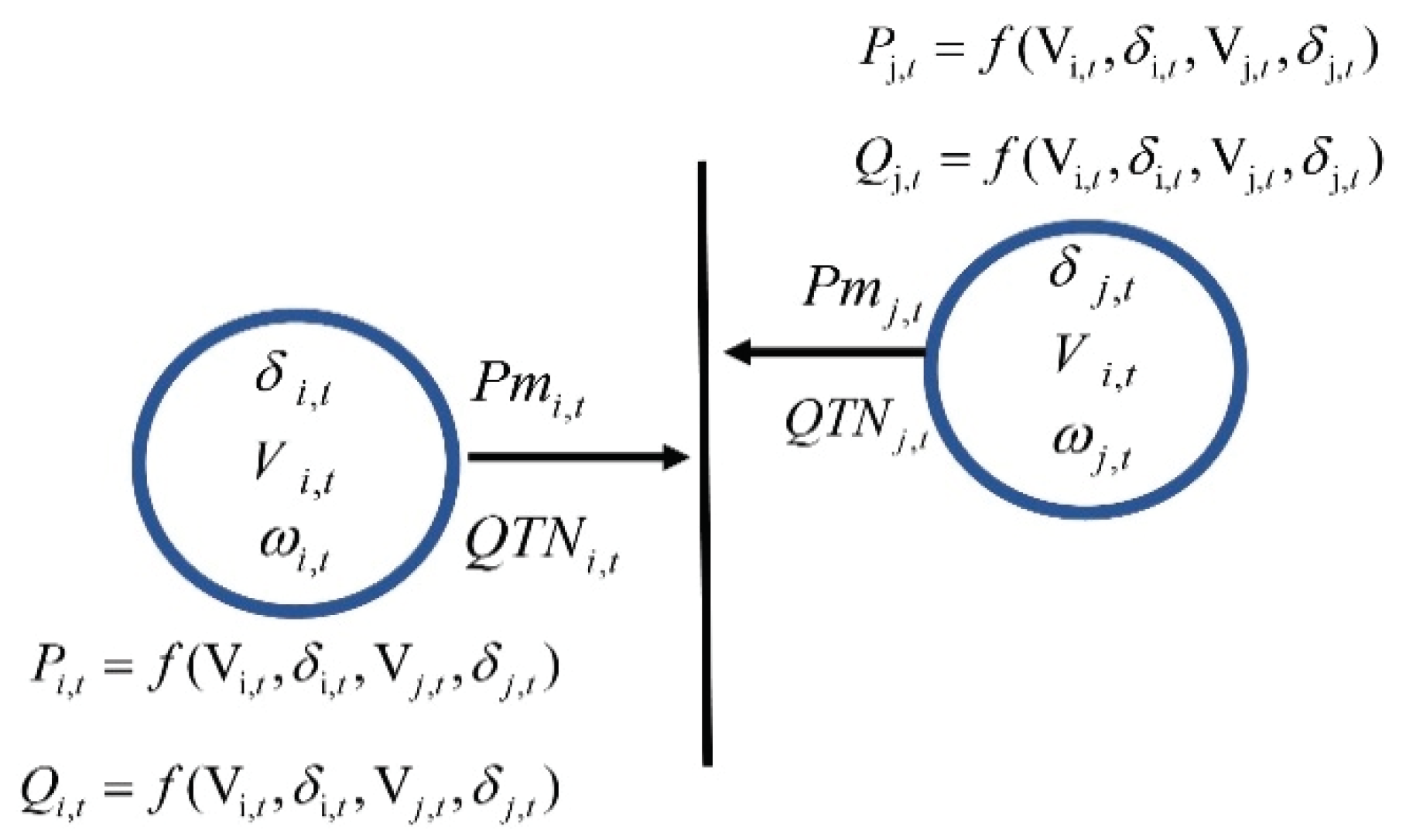
The decision variables are:

• $P_{i,t}\hspace{0.17em}\hspace{0.17em}i\in A\hspace{0.17em},\hspace{0.17em}\hspace{0.17em}t=0,\dots ,T-1$: active power injected at node i.
• $Q_{i,t}\hspace{0.17em}\hspace{0.17em}i\in A\hspace{0.17em},\hspace{0.17em}\hspace{0.17em}t=0,\dots ,T-1$: reactive power injected at node i.
• $P{G}_{i,t}\hspace{0.17em}\hspace{0.17em}i\in A\hspace{0.17em},\hspace{0.17em}\hspace{0.17em}\hspace{0.17em}\hspace{0.17em}t=0,\dots ,T-1$: distributed controllable source active power at node i.
• $QN{G}_{i,t}\hspace{0.17em}\hspace{0.17em}i\in A\hspace{0.17em},\hspace{0.17em}\hspace{0.17em}\hspace{0.17em}\hspace{0.17em}t=0,\dots ,T-1$: reactive power regulating source reactive power at node i.
• $P{m}_{i,t}$: regulation active power injected by local system i.
• $V_{i,t}\hspace{0.17em}\hspace{0.17em}\hspace{0.17em}i\in A\hspace{0.17em},\hspace{0.17em}\hspace{0.17em}t=0,\dots ,T-1$: voltage amplitude at node i

The parameters are:

• $P{L}_{i,t}\hspace{0.17em}\hspace{0.17em}i\in A\hspace{0.17em},\hspace{0.17em}\hspace{0.17em}\hspace{0.17em}\hspace{0.17em}t=0,\dots ,T-1$: load active power at node i.
• $Q{L}_{i,t}\hspace{0.17em}\hspace{0.17em}i\in A\hspace{0.17em},\hspace{0.17em}\hspace{0.17em}\hspace{0.17em}\hspace{0.17em}t=0,\dots ,T-1$: load reactive power at node i.
• $Q{G}_{i,t}\hspace{0.17em}\hspace{0.17em}i\in A\hspace{0.17em},\hspace{0.17em}\hspace{0.17em}\hspace{0.17em}\hspace{0.17em}t=0,\dots ,T-1$: distributed controllable source reactive power at node i.
• $PN{G}_{i,t}\hspace{0.17em}\hspace{0.17em}i\in A\hspace{0.17em},\hspace{0.17em}\hspace{0.17em}\hspace{0.17em}\hspace{0.17em}t=0,\dots ,T-1$: reactive power regulating source active power at node i.
• $PRE{S}_{i,t}\hspace{0.17em}\hspace{0.17em}i\in A\hspace{0.17em},\hspace{0.17em}\hspace{0.17em}\hspace{0.17em}\hspace{0.17em}t=0,\dots ,T-1$: renewable source active power at node i.
• $QRE{S}_{i,t}\hspace{0.17em}\hspace{0.17em}i\in A\hspace{0.17em},\hspace{0.17em}\hspace{0.17em}\hspace{0.17em}\hspace{0.17em}t=0,\dots ,T-1$: renewable source reactive power at node i.

The state variables are:

• ${\delta }_{i,t}\hspace{0.17em}\hspace{0.17em}\hspace{0.17em}\hspace{0.17em}i\in A\hspace{0.17em},\hspace{0.17em}\hspace{0.17em}t=0,\dots ,T-1$: voltage phase at node i (rad).
• ${\omega }_{i,t}\hspace{0.17em}\hspace{0.17em}i\in A\hspace{0.17em},\hspace{0.17em}\hspace{0.17em}t=0,\dots ,T-1$: frequency at node i.

The decision variables detail for a local system is reported in Figure 2.

The electrical grid inside each local system i is not considered, and thus only the power balance must be satisfied:

$$P{G}_{i,t}+PN{G}_{i,t}+PRE{S}_{i,t}-P{L}_{i,t}=P_{i,t}\hspace{0.17em}\hspace{0.17em}\hspace{0.17em}i\in A\hspace{0.17em},\hspace{0.17em}\hspace{0.17em}\hspace{0.17em}t=0,\dots ,T-1$$

(1)

$$Q{G}_{i,t}+QN{G}_{i,t}+QRE{S}_{i,t}-Q{L}_{i,t}=Q_{i,t}\hspace{0.17em}\hspace{0.17em}\hspace{0.17em}i\in A\hspace{0.17em},\hspace{0.17em}\hspace{0.17em}\hspace{0.17em}t=0,\dots ,T-1$$

(2)

Each local system is associated with a time-varying voltage phasor of magnitude $V_{i,t}$ and phase ${\delta }_{i,t}$. The discrete-time system dynamics ($\Delta t$ is the time interval length) are governed by the equations of the virtual inertia controller, linking the node angle, ${\delta }_{i,t}$, to the frequency difference to the nominal value (${\omega }_{i,t}$ − ${\omega }_0$):

$${\delta }_{i,t+1}={\delta }_{i,t}+({\omega }_{i,t}-{\omega }_0)\Delta t\hspace{0.17em}\hspace{0.17em}\hspace{0.17em}\hspace{0.17em}i\in A\hspace{0.17em}\hspace{0.17em}\hspace{0.17em}\hspace{0.17em}t=0,\dots ,T-1$$

(3)

where the frequency is related to the active power supply–demand imbalance:

$${\omega }_{i,t+1}={\omega }_{i,t}+\frac{P{m}_{i,t}-P{G}_{i,t}-K{D}_i({\omega }_{i,t}-{\omega }_0)}{2H_i}\Delta t\hspace{1em}i\in A\hspace{0.17em},\hspace{0.17em}\hspace{0.17em}t=0,\dots ,T-1$$

(4)

where $K{D}_i$ is the local system damping factor. The distribution grid model includes the linearized power flow equations for a medium voltage AC grid, with $G_{i,j}=1/R_{i,j}\hspace{0.17em}\hspace{0.17em}\hspace{0.17em}\left(i,j\in A\right)$ as the line conductance, and $B_{i,j}=-1/X_{i,j}\hspace{0.17em}\hspace{0.17em}\hspace{0.17em}\left(i,j\in A\right)$ as the line susceptance. That is:

$$P_{i,t}={\displaystyle \sum _{j\in A}{G}_{i,j}{V}_{j,t}+B_{i,j}\left({\delta }_{i,t}-{\delta }_{j,t}\right)\hspace{0.17em}\hspace{0.17em}}\hspace{0.17em}\hspace{0.17em}i,j\in A\hspace{0.17em}\hspace{0.17em}\hspace{0.17em}\hspace{0.17em}t=0,\dots ,T-1$$

(5)

$$Q_{i,t}={\displaystyle \sum _{j\in A}-B_{i,j}{V}_{j,t}+G_{i,j}\left({\delta }_{i,t}-{\delta }_{j,t}\right)\hspace{0.17em}\hspace{0.17em}}\hspace{0.17em}\hspace{0.17em}i,j\in A\hspace{0.17em}\hspace{0.17em}\hspace{0.17em}\hspace{0.17em}t=0,\dots ,T-1$$

(6)

The model described by Equations (5) and (6) is the well-known linearized version of power flow equations, obtained considering the first term of Taylor expansion of the sinusoidal terms of the equations and just considering the voltage difference between nodes [42,43,44].

In the following paragraphs, the linear model described by the previous equations is reformulated in the state space canonical form.

Proposition I: The system model, described by Equations (1)–(6), can be expressed as an affine system affected by additive noise:

$$x_{t+1}=A{x}_t+B{u}_t+C{h}_t+\widehat{C}{\widehat{h}}_t\hspace{1em}t=0,\dots ,T-1$$

(7)

with

• $u_t=[P{m}_{i,t},i=1,\dots ,N-1,QT{N}_{i,t},i=1,\dots ,N-1],$
• $x_t=[{\delta }_{i,t},i=1,\dots ,N-1;{\omega }_{i,t},i=1,\dots ,N-1]$,

where A, B, C, and $\widehat{C}$ are known matrices, $h_t$ is a vector of parameters, and ${\widehat{h}}_t$ represents stochastic noise with $E\left\{{\widehat{h}}_t\right\}=0$.

Proof of Proposition I: The Proof is shown in the Appendix A.1.

In the day ahead, the DSO plans the production and energy flow based on different objectives, such as the minimization of losses and the capacity of the lines. It is reasonable to consider variations concerning an already predetermined working point. However, given the strong variability of part of the energy sources involved in our problem, control policies are required to mitigate deviations from an initial working point.

The proposed objective function aims at minimizing four different contributions: the square of the difference between the phases of the grid nodes, the quadratic deviation of the frequency from the steady-state value, the voltage quadratic deviation from the desired value, $V_0$, and the quadratic deviation of the active regulation power to the set point $P{m}^{\ast }$:

$$\min \hspace{0.17em}\hspace{0.17em}\left[\left({\displaystyle \sum _{t=0}^T{\displaystyle \sum _{\begin{array}{l}i,j\in A\\ i\ne j\end{array}}{\left({\delta }_{i,t}-{\delta }_{j,t}\right)}^2}}\right)+\left({\displaystyle \sum _{t=0}^T{\displaystyle \sum _{i\in A}{\left({\omega }_{i,t}-{\omega }_0\right)}^2}}\right)+\left({\displaystyle \sum _{t=0}^{T-1}{\displaystyle \sum _{i\in A}{\left(V_{i,t}-V_0\right)}^2}}\right)+\left({\displaystyle \sum _{t=0}^{T-1}{\displaystyle \sum _{i\in A}{\left(P{m}_{i,t}-P{m}_i^{\ast }\right)}^2}}\right)\right]$$

(8)

Proposition II: The objective function (8) can be expressed as a stochastic quadratic function with mixed terms:

$$\min J\left(x_t,u_t\right)=\frac{1}{2}E\left\{{\displaystyle \sum _{t=0}^{T-1}\left[\begin{array}{l}{\left(x_t-\widehat{x}\right)}^{\prime }{Q}_t\left(x_t-\widehat{x}\right)+{\left(u_t-{\widehat{u}}_t\right)}^{\prime }{R}_t\left(u_t-{\widehat{u}}_t\right)\\ +2{\left(x_t-\widehat{x}\right)}^{\prime }{F}_t{\left(u_t-{\widehat{u}}_t\right)}^{\prime }\end{array}\right]+{\left(x_T-\widehat{x}\right)}^{\prime }{Q}_T\left(x_T-\widehat{x}\right)}\right\}$$

(9)

where $x_t$ and $u_t$ are the state and control vectors respectively, $\widehat{x},\widehat{u}$ are the tracking parameters, and Q_t, R_t, F_t , Q_T are known matrices.

Proof of Proposition II: The Proof is shown in the Appendix A.2.

4. The Model Predictive Control Problem

4.1. The MPC Scheme

The MPC scheme is defined in Figure 3. The optimization horizon (T) is the length over which the optimization problem runs and (S) is the simulation horizon. Both horizons (T) and (S) can be chosen according to the available information about uncertain parameters/forecasts (current states, forecasted demands, and renewables). In the MPC approach, in the first run, the solution related to the first time interval is considered. Then, uncertain parameters (new information from sensors in the field and new forecasts) are inserted in the procedure and a new optimization problem is run (second run), and so on for the whole duration of the simulation horizon (S). The MPC approach allows for updating new information when available and reducing uncertainties related to renewables’ availability and load forecasting.

4.2. Explicit Solution of the MPC Problem

The optimization problem is in the form:

$$\min J\left(x_t,u_t\right)=\frac{1}{2}E\left\{{\displaystyle \sum _{t=0}^{T-1}\left[\begin{array}{l}{\left(x_t-\widehat{x}\right)}^{\prime }{Q}_t\left(x_t-\widehat{x}\right)+{\left(u_t-{\widehat{u}}_t\right)}^{\prime }{R}_t\left(u_t-{\widehat{u}}_t\right)\\ +2{\left(x_t-\widehat{x}\right)}^{\prime }{F}_t{\left(u_t-{\widehat{u}}_t\right)}^{\prime }\end{array}\right]+{\left(x_T-\widehat{x}\right)}^{\prime }{Q}_T\left(x_T-\widehat{x}\right)}\right\}$$

(10)

subject to (s.t.) Equation (7).

By a change of variables $z_t=x_t-\widehat{x}$ and $e_t=u_t-{\widehat{u}}_t$, the optimization problem is given by:

$$\min J\left(z,e\right)=\frac{1}{2}E\left\{{\displaystyle \sum _{t=0}^{T-1}\left[z_t^{\prime }{Q}_t{z}_t+e_t^{\prime }{R}_t{e}_t+2z_t^{\prime }{F}_t{e}_t\right]+z_T^{\prime }{Q}_T{z}_T}\right\}$$

(11)

s.t.

$$z_{t+1}=A{z}_t+B{e}_t+{\mu }_t+\widehat{C}{\widehat{h}}_t\hspace{1em}t=0,\dots ,T-1$$

(12)

where:

$${\mu }_t=C{h}_t+\left(A-I\right)\widehat{x}+B{\widehat{u}}_t\hspace{1em}t=0,\dots ,T-1$$

(13)

The Equations (11)–(13) are a stochastic MPC problem, which is “non-standard,” due to the presence of the known input sequence, ${\mu }_t$, in the state equation. In the following claims, it is shown how to solve the MPC problem in a closed-form through a two-stage decomposition.

Claim I: Due to its linearity, the decision problem in Equations (11)–(13) can be decomposed separating the stochastic ($z_{t+1}^s$) and deterministic ($z_{t+1}^d$) components [45]:

$$J\left(z,e\right)=J\left(z^s,e^s\right)+J\left(z^d,e^d\right)$$

(14)

s.t.

$$z_{t+1}^s=A{z}_t^s+B{e}_t^s+\widehat{C}{\widehat{h}}_t\hspace{1em}t=0,\dots ,T-1$$

(15)

$$z_0^s=0$$

(16)

$$z_{t+1}^d=A{z}_t^d+B{e}_t^d+{\mu }_t\hspace{1em}\hspace{1em}t=0,\dots ,T-1$$

(17)

$$z_0^d=z_0$$

(18)

The optimal control strategy is given by:

$$z_t^{\ast }=z_t^{s,\ast }+z_t^{d,\ast }\hspace{1em}\hspace{1em}t=0,\dots ,T-1$$

(19)

$$e_t^{\ast }=e_t^{s,\ast }+e_t^{d,\ast }\hspace{1em}t=0,\dots ,T-1$$

(20)

Proof of Claim I: The Proof is shown in the Appendix A.3.

Claim II: The optimal control problem to determine $e_t^{d,\ast }$, due to its linearity, can be written as:

$$\min J\left(z^d,e^d\right)=\frac{1}{2}E\left\{{\displaystyle \sum _{t=0}^{T-1}{\left(z_t^{d1}-r_t\right)}^{\prime }{Q}_t\left(z_t^{d1}-r_t\right)+{e_t^d}^{\prime }{R}_t{e}_t^d+2{\left(z_t^{d1}-r_t\right)}^{\prime }{F}_t{e}_t^d+{\left(z_T^{d1}-r_T\right)}^{\prime }{Q}_T\left(z_T^{d1}-r_T\right)}\right\}$$

(21)

where:

$$z_t^d=z_t^{d1}+z_t^{d2}\hspace{1em}t=0,\dots ,T-1$$

(22)

$$z_{t+1}^{d1}=A{z}_t^{d1}+B{e}_t^d\hspace{1em}t=0,\dots ,T-1$$

(23)

$$z_0^{d1}=0$$

(24)

$$z_{t+1}^{d2}=A{z}_t^{d2}+{\mu }_t\hspace{1em}t=0,\dots ,T-1$$

(25)

$$z_0^{d2}=z_0$$

(26)

$$z_t^{d2}=-r_t\hspace{1em}t=0,\dots ,T-1$$

(27)

Proof of Claim II: The Proof is shown in the Appendix A.4.

Proposition III: The optimal control law for the problem in Equations (11)–(13), and taking into account Claim I and Claim II, is given by:

$$e_t^{\ast }=-K_t(z_t^s+z_t^{d1})+K_t^g(B^{\prime }{g}_{t+1}+{F_t}^{\prime }{r}_t)\hspace{1em}t=0,\dots ,T-1$$

(28)

with

$$\begin{gathered} g_t=-\left[\left(A^{\prime }-{M_t}^{\prime }\right)P_{t+1}{\left(I+E_t{P}_{t+1}\right)}^{-1}\left(E_t{g}_{t+1}+M_t{r}_t\right)-\left(A^{\prime }-{M_t}^{\prime }\right)g_{t+1}\right]+(Q_t-D_t)r_t \\ t=0,\dots ,T-1 \end{gathered}$$

(29)

$$K_t={\left(R+B^{\prime }{P}_{t+1}B\right)}^{-1}\left(B^{\prime }{P}_{t+1}A+{F_t}^{\prime }\right)\hspace{1em}t=0,\dots ,T-1$$

(30)

$$P_t=Q_t-D_t+\left(A^{\prime }-{M_t}^{\prime }\right)P_{t+1}{\left(I+E_t{P}_{t+1}\right)}^{-1}\left(A_t-M_t\right)\hspace{1em}t=0,\dots ,T-1$$

(31)

$$K_t^g={\left(R_t+B^{\prime }{P}_{t+1}B\right)}^{-1}\hspace{1em}t=0,\dots ,T-1$$

(32)

$$r_{t+1}=A{r}_t-{\mu }_t$$

(33)

$$P_T=Q_T\hspace{1em}t=0,\dots ,T-1$$

(34)

$$g_T=Q_T{r}_T\hspace{1em}t=0,\dots ,T-1$$

(35)

being: $M_t=B{R}_t^{-1}{F_t}^{\prime }$, $D_t=F_t{R}_t^{-1}{F_t}^{\prime }$, $D_t=F_t{R}_t^{-1}{F_t}^{\prime }$ and $E_t=B{R}_t^{-1}{B}^{\prime }$.

Proof of Proposition III: The Proof is shown in the Appendix A.5.

As reported in Claim I and Claim II, the original problem can be so decomposed into a stochastic problem and a deterministic discrete tracking problem. The closed-loop optimal control strategy is obtained as follows [46]:

Sub-problem 1: Stochastic problem.

The optimal control problem to determine $e_t^{s,\ast }$ is given by:

$$\min J\left(z,e\right)=\frac{1}{2}E\left\{{\displaystyle \sum _{t=0}^{T-1}\left[{z_t^s}^{\prime }{Q}_t{z}_t^s+{e_t^s}^{\prime }{R}_t{e}_t^s+2{z_t^s}^{\prime }{F}_t{e}_t^s\right]+{z_T^s}^{\prime }{Q}_T{z}_T^s}\right\}$$

(36)

s.t.

$$z_{t+1}^s=A{z}_t^s+B{e}_t^s+\widehat{C}{\widehat{h}}_t\hspace{1em}t=0,\dots ,T-1$$

(37)

$$z_0^s=0\hspace{1em}t=0,\dots ,T-1$$

(38)

Proposition IV: The solution of the optimal control problem, Equations (36)–(38), is given by the following recursive equations:

$$e_t^{s\ast }=-K_t{z}_t^{s\ast }\hspace{1em}t=0,\dots ,T-1$$

(39)

with

$$K_t={\left(R+B^{\prime }{P}_{t+1}B\right)}^{-1}\left(B^{\prime }{P}_{t+1}A+{F_t}^{\prime }\right)\hspace{1em}t=0,\dots ,T-1$$

(40)

$$P_t=Q_t-D_t+\left(A^{\prime }-{M_t}^{\prime }\right)P_{t+1}{\left(I+E_t{P}_{t+1}\right)}^{-1}\left(A_t-M_t\right)\hspace{1em}t=0,\dots ,T-1$$

(41)

$$P_T=Q_T$$

(42)

being $M_t=B{R}_t^{-1}{F_t}^{\prime }$,$D_t=F_t{R}_t^{-1}{F_t}^{\prime }$ and $E_t=B{R}_t^{-1}{B}^{\prime }$.

Proof of Proposition IV: The Proof is shown in the Appendix A.6.

Sub-problem 2: Deterministic problem.

As reported in Claim II, the optimal control problem to determine $e_t^{d,\ast }$ can be written as:

$$\min J\left(z^d,e^d\right)=\frac{1}{2}E\left\{{\displaystyle \sum _{t=0}^{T-1}\left[{\left(z_t^{d1}-r_t\right)}^{\prime }{Q}_t\left(z_t^{d1}-r_t\right)+{e_t^d}^{\prime }{R}_t{e}_t^d+2{\left(z_t^{d1}-r_t\right)}^{\prime }{F}_t{e}_t^d\right]+{\left(z_T^{d1}-r_T\right)}^{\prime }{Q}_T\left(z_T^{d1}-r_T\right)}\right\}$$

(43)

s.t.

$$z_{t+1}^{d1}=A{z}_t^{d1}+B{e}_t^d\hspace{1em}t=0,\dots ,T-1$$

(44)

$$z_0^{d1}=0$$

(45)

being $z_t^{d2}=-r_t$, $z_0^{d2}=z_0$, $z_{t+1}^{d2}=A{z}_t^{d2}+{\mu }_t$, ${\mu }_t=C{h}_t+\left(A-I\right)\widehat{x}+B{\widehat{u}}_t$.

Proposition V: The optimal control strategy for the problem, Equations (43)–(45), is given by

$$e_k^{d,\ast }=-K_t{z}_t^{d1}+K_t^g\left(B^{\prime }{g}_{t+1}+{F_t}^{\prime }{r}_t\right)\hspace{1em}t=0,\dots ,T-1$$

(46)

with

$$\begin{gathered} g_t=-\left[\left(A^{\prime }-{M_t}^{\prime }\right)P_{t+1}{\left(I+E_t{P}_{t+1}\right)}^{-1}\left(E_t{g}_{t+1}+M_t{r}_t\right)-\left(A^{\prime }-{M_t}^{\prime }\right)g_{t+1}\right]+(Q_t-D_t)r_t \\ t=0,\dots ,T-1 \end{gathered}$$

(47)

$$K_t={\left(R_t+B^{\prime }{P}_{t+1}B\right)}^{-1}\left(B^{\prime }{P}_{t+1}A+{F_t}^{\prime }\right)\hspace{1em}t=0,\dots ,T-1$$

(48)

$$K_t^g={\left(R_t+B^{\prime }{P}_{t+1}B\right)}^{-1}\hspace{1em}t=0,\dots ,T-1$$

(49)

$$P_t=Q_t-D_t+\left(A^{\prime }-{M_t}^{\prime }\right)P_{t+1}{\left(I+E_t{P}_{t+1}\right)}^{-1}\left(A-M_t\right)\hspace{1em}t=0,\dots ,T-1$$

(50)

$$r_{t+1}=A{r}_t-{\mu }_t\hspace{1em}t=0,\dots ,T-1$$

(51)

$$P_T=Q_T$$

(52)

$$g_T=Q_T{r}_T$$

(53)

5. Application to a Case Study

5.1. Case Study Description

To show the effectiveness of the theoretical results presented in the previous section, the proposed control strategy has been applied to a modified IEEE 5-bus system (N = 5) [47], shown in Figure 4. The test network has been adapted to our problem through the following assumptions. Each bus corresponds to a local system, and, keeping the network topology unchanged, the values of cables’ resistance, R_i,j, and reactance, X_i,j, have conveniently rescaled to a distribution grid system (assuming base quantities of 10 MVA for apparent power, $V_0$= 15 KV for voltage and ${\omega }_0$= 50 Hz for frequency).

Table 1. Lines data.

Line	Resistance Ri,j (p.u.)	Reactance Xi,j (p.u.)
1–2	0.088	0.266
1–3	0.355	1.066
2–3	0.266	0.800
2–4	0.266	0.800
2–5	0.177	0.533
3–4	0.177	0.533
4–5	0.355	1.066

shows the detailed values of the line parameters R_i,j, and X_i,j for the case study.

The parameters that characterize each local system, i.e., the inertia constant, H_i, and the equivalent damping factor, KD_i, are reported in

Table 2. Local systems’ parameters.

Parameter	Local System 1	Local System 2	Local System 3	Local System 4
KDi (p.u)	3	4	3.5	5
Hi (s)	5	4	5.5	6

. The local system 5 is the slack node, in which the voltage, $V_{5,t}$, is fixed to 1 (p.u.) and the phase, ${\delta }_{5,t}$, is equal to 0 (rad). The case study can be representative of small local systems connected by a distribution grid (such as interconnected microgrids), in which there is a great presence of generation from renewable resources.

The simulation horizon is 60 s, with a discretization step $\Delta t$ of 0.5 s. This horizon length has been chosen as a trade-off between the following two aspects: (a) to avoid delays due to the centralized communication from the controller to the local systems, and (b) to enhance the reliability of the short-term forecasting of RES and loads.

To make the approach more effective, the MPC strategy is applied, in which only a part of the optimal control law is applied (e.g., 10 seconds over a T = 60 second horizon), and there is a continuous recalculation of the control law based on new measurements and forecasting. The length of the MPC control horizon is justified by recent developments on the nowcasting of renewable power sources that predict 1 min future PV values [48,49].

At this point, by the means of the local systems’ parameters and the distribution network, it is possible to quantify the matrices A and B, defined in the Appendix A.1, described by Equations (A19) and (A20), and needed by Equation (7):

$$A=\left(\begin{array}{cccccccc}1& 0& 0& 0& 0.5& 0& 0& 0\\ 0& 1& 0& 0& 0& 0.5& 0& 0\\ 0& 0& 1& 0& 0& 0& 0.5& 0\\ 0& 0& 0& 1& 0& 0& 0& 0.5\\ -0.22& 0.21& 3.8\mathrm{e}-19& 0.035& 0.76& 0& 0& 0\\ 0.16& -0.47& 0.062& 0.046& 0& 0.66& 0& 0\\ -2.08\mathrm{e}-18& 0.07& -0.54& 0.070& 0& 0& 0.58& 0\\ 0.0421& 0.07& 0.093& -0.20& 0& 0& 0& 0.80\end{array}\right)$$

$$B=\left(\begin{array}{cccccccc}0& 0& 0& 0& 0& 0& 0& 0\\ 0& 0& 0& 0& 0& 0& 0& 0\\ 0& 0& 0& 0& 0& 0& 0& 0\\ 0& 0& 0& 0& 0& 0& 0& 0\\ 0.05& 0& 0& 0& 0.33& 0& -6.93\mathrm{e}-18& -2.77\mathrm{e}-17\\ 0& 0.062& 0& 0& 0& 0.33& 4.51\mathrm{e}-17& 6.93\mathrm{e}-17\\ 0& 0& 0.055& 0& 4.6\mathrm{e}-17& 5.55\mathrm{e}-17& 0.33& 2.77\mathrm{e}-17\\ 0& 0& 0& 0.041& -5.55\mathrm{e}-17& 2.77\mathrm{e}-17& -1.38\mathrm{e}-17& 0.33\end{array}\right)$$

In each MPC step, the optimal control law is the sum of the solution of two different control problems: a stochastic problem defined by Equations (36)–(38), with the optimal solution, Equations (39)–(42), and a deterministic problem, Equations (43)–(45), with the optimal solution, Equations (46)–(53). Both control laws have been recursively defined, i.e., all the parameters that define the control can be calculated offline, the parameters are known, and the forecasts of renewable generation and load.

The variations on the system are caused by the combined variation of load and RES Psc_,i,t on the local systems defined by Equation (A4), represented into the model in the terms $h_t$ and ${\widehat{h}}_t$ defined by Equations (A21) and (A22) respectively, deterministic and stochastic parts of the noise. Figure 5 reports the values, $Ps{c}_{i,t}^d$, for the whole simulation horizon. Data have been obtained by adapting real power measurements from photovoltaic, residential, and industrial loads, and rescaled to obtain congruent measurements for the distribution networks. The stochastic part of the noise, $Ps{c}_{i,t}^s$~ N(0,1), affects the state at each instant t.

The power profiles on each local system could be critical for the whole system. Without any upper-level controller but only with the damping given by each local system, the generators could not be able to efficiently compensate (i.e., in a reasonable time, according to the dynamics of the system) the given power variation, causing frequency and voltage variations.

The objective of the proposed controller is to reduce the voltage and frequency variations (during the transient period) and, after the perturbation, bringing them back to their reference value. In a practical context, numerous frequency variations and voltage peaks on the grid could cause the intervention of protection systems, sensitive to variations in voltage or frequency, disconnecting some portions of the network itself, causing a blackout for many users.

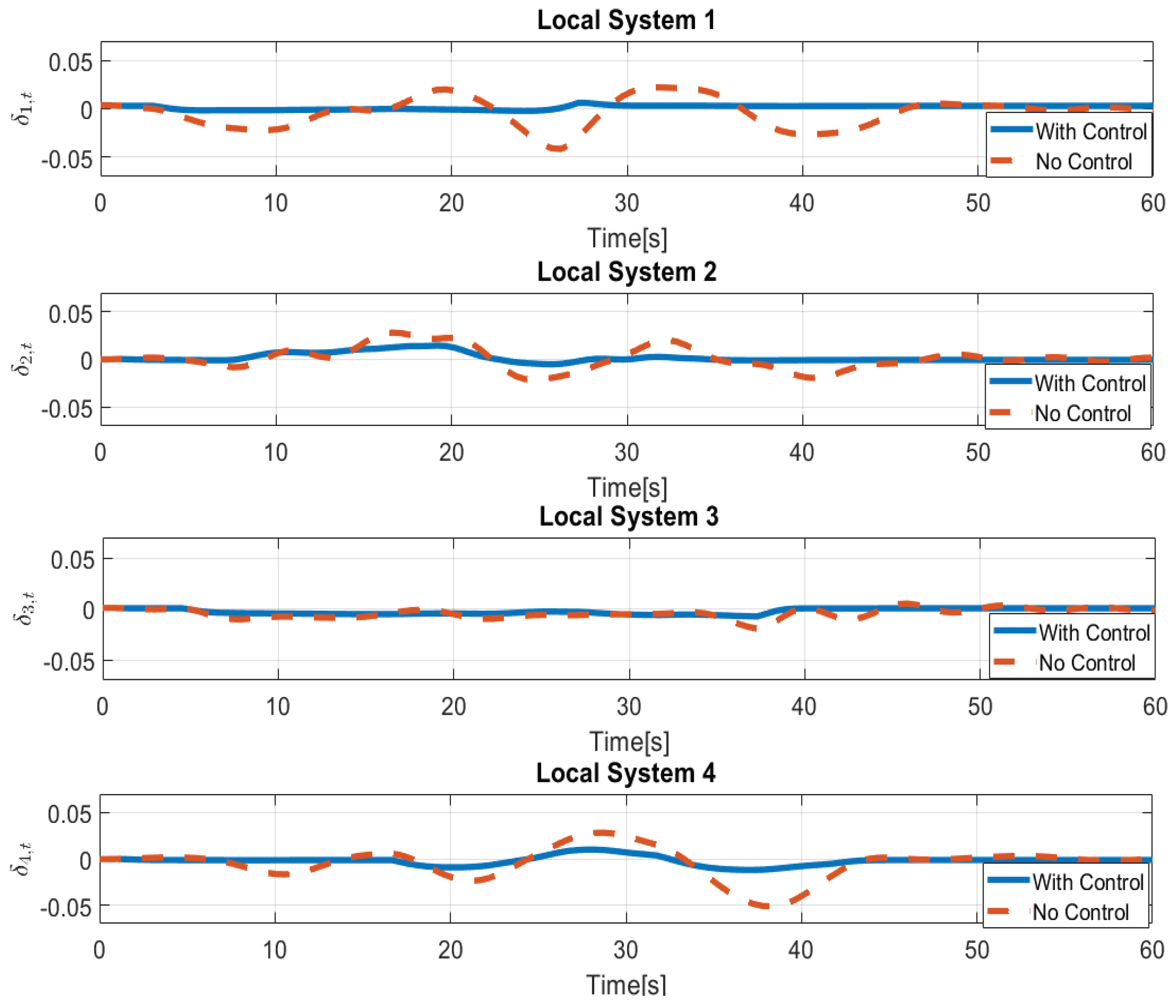
5.2. Optimal Control Results

Optimal solutions for the state variables in the case with control or without control are reported in Figure 6 and Figure 7. It can be seen how the presence of the proposed control can limit frequency variations (i.e., the power quality remains within acceptable limits, the voltage deviation from the reference value is less than 5%). The dotted line represents the system with no control (only the damping coefficient is considered). In this case, each local system operates without any central controller (like the one developed here), but the system only reacts based on the physics of the system with constant inputs equal to those of the equilibrium point. The bold line represents the controlled system using the developed approach. It is important to note that without the proposed control strategy, the system does not reach a steady state for the whole simulation.

Figure 8 shows the voltage pattern for each local system in the presence or absence of the developed control. The control strategy helps in containing the variations affecting this variable, improving the system’s power quality. Finally, Figure 9 and Figure 10 show the optimal active and reactive power at each local system.

When there is no control, the objective function value is equal to 0.1098, while when the proposed control strategy is applied, it is 0.0151.

Table 3. Objective function values and contributions.

Contribution	Phase	Frequency	Voltage	Active Power
No Control	0.00854	8.71 × −4	0.0095	0
With Control	0.00853	8.64 × −4	0.0042	0.0015

shows the objective function values and contributions.

The test has been developed in MATLAB-SIMULINK (2018b, Mathworks, Natick, Massachusetts, USA), running on a PC Intel i7, 16 GB RAM. The MATLAB tool has been used to calculate a priori the control laws defined recursively in Section 4.

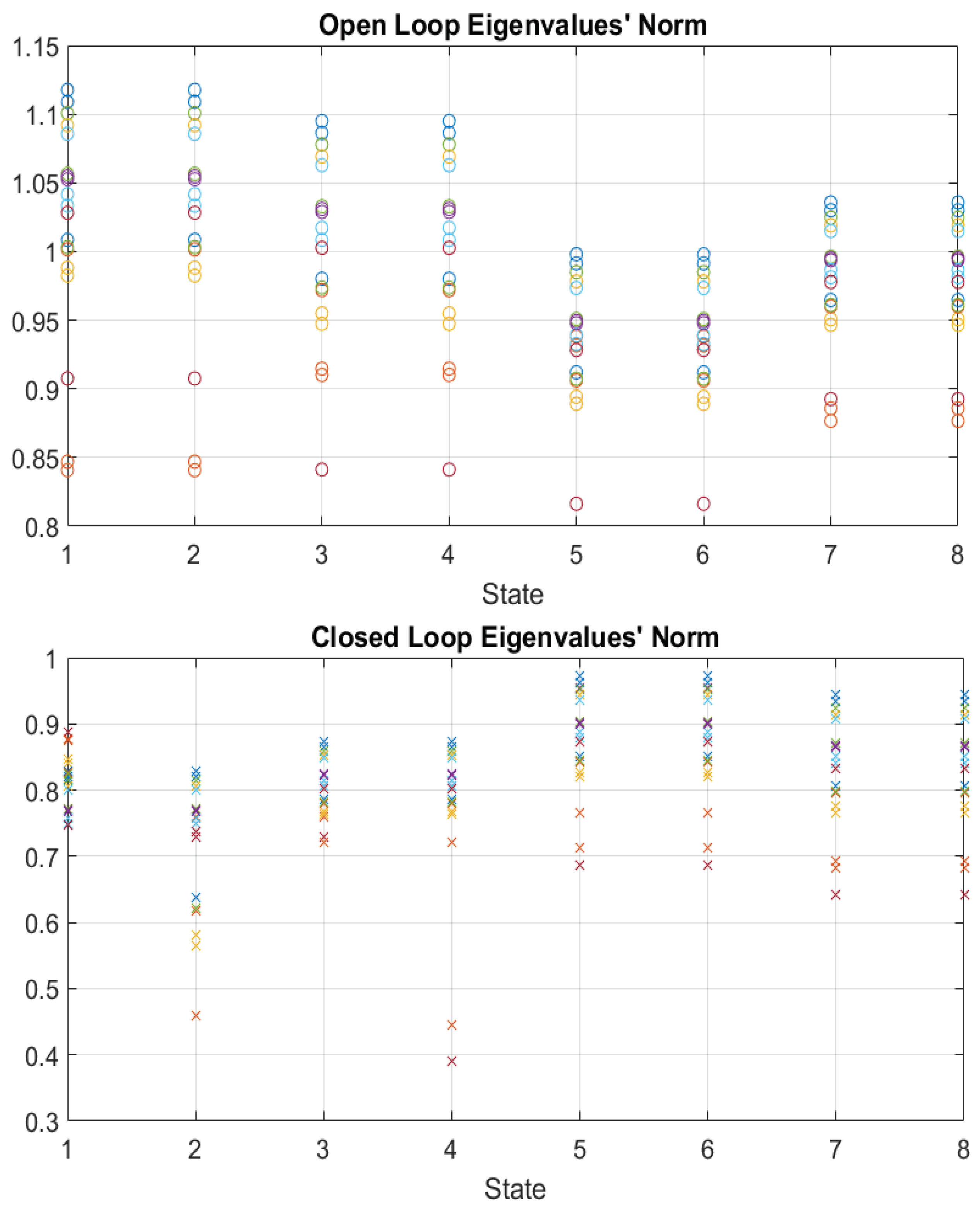
5.3. Closed-Loop Stability Analysis

This subsection aims to perform a sensitivity analysis concerning the asymptotic stability properties of the proposed system, with respect to the damping parameter, KD_i. The choice of this parameter is fundamental with regards to the design of the control system based on virtual inertia. It is well known from power systems theory that the asymptotic stability of a synchronous machine is directly linked to its damping factor, similarly for the virtual inertia that mimics this behavior.

The first part of Figure 11 shows how different choices of damping factors at each node affect the norm of the eigenvalues of the open-loop system for each element of the state vector $x$. The values are chosen in an interval between $\pm 50\%$ of the ones used for the use case, 20 different damping factors are considered.

It is noteworthy that for lower values of KD_i, some eigenvalues have a norm greater than 1, so the system is unstable. This is consistent with the power system theory. To this end, the asymptotical closed-loop stability of the proposed controller for an infinite time control law defined is analyzed, as in Reference . As can be seen from the second part of Figure 11, the proposed optimal controller also guarantees the asymptotical stability in the cases in which the system was designed as unstable. This aspect is crucial for the optimal control of this kind of problem, as it also fixes design instabilities.

6. Conclusions and Future Developments

The proposed work introduced an approach based on optimal control for the regulation of voltage and frequency in multi-local systems (such as interconnected microgrids) in a distribution grid. This represents one of the most challenging problems regarding the dynamic aspects of a smart grid.

If not considered and properly mitigated, these aspects can drastically damage the entire system. To reduce these effects, the paper considers accurate grid models and the presence of innovative devices that allow for better regulating the power flows on the grid and, consequently, voltage and frequency at each node. It is worthwhile to observe that the main contribution of this paper is not to assess the controller performance (that is optimal by definition to the linearized model) but to propose a model that can be linearized and controlled by a closed-form control law.

To cope with the variability represented by renewable sources and load, this approach was used in an MPC framework. In this case, just the control law corresponding to the first time interval would be applied, while an update of the law would be performed according to the new forecasts made in the short term. This would allow a further increase in the quality of the system. The IEEE 5 bus system was used to test the control strategy, considering multiple loads and renewable sources variations on each local system. The results showed a strong decrease in the number of variations as well as strong damping of the frequency and voltage peaks in each local system. This greatly increases the power quality of the electrical system. A sensitivity analysis about the asymptotical stability was also given, showing that the proposed control can also prevent instabilities caused by an incorrect design of the damping parameters.

Future developments will concern several aspects. First, delays in the communication between the central controller and each local system could be inserted in the optimal control problem.

The particular model of the local systems will be the focus of future investigations. Furthermore, distributed and team robust approaches to overcome the poor robustness of totally centralized control approaches in case of emergencies will be considered.

References

1. Arya, Y.; Kumar, N. Optimal control strategy-based AGC of electrical power systems: A comparative performance analysis. Optim. Control Appl. Methods 2017, 38, 982–992. [Google Scholar] [CrossRef]
2. Dagdougui, H.; Ouammi, A.; Sacile, R. Optimal control of a networkof power microgrids using the Pontryagin’s minimum principle. IEEE Trans. Control Syst. Technol. 1942, 22, 1942–1948. [Google Scholar] [CrossRef]
3. Bersani, C.; Dagdougui, H.; Ouammi, A.; Sacile, R. Distributed Robust Control of the Power Flows in a Team of Cooperating Microgrids. IEEE Trans. Control Syst. Technol. 2016, 25, 1473–1479. [Google Scholar] [CrossRef]
4. Ferro, G.; Minciardi, R.; Parodi, L.; Robba, M.; Rossi, M. Optimal Control of Multiple Microgrids and Buildings by an Aggregator. Energies 2020, 13, 1058. [Google Scholar] [CrossRef] [Green Version]
5. Pandey, R.K.; Gupta, D.K. Intelligent Multi-Area Power Control: Dynamic Knowledge Domain Inference Concept. IEEE Trans. Power Syst. 2017, 32, 4310–4318. [Google Scholar] [CrossRef]
6. Trip, S.; Cucuzzella, M.; De Persis, C.; Ferrara, A.; Scherpen, J.M. Robust load frequency control of nonlinear power networks. Int. J. Control 2018, 93, 346–359. [Google Scholar] [CrossRef]
7. Datta, S. Small Signal Stability Criteria for Descriptor Form Power Network Model. Int. J. Control 2018, 2018, 1–16. [Google Scholar] [CrossRef]
8. Dreidy, M.; Mokhlis, H.; Mekhilef, S. Inertia response and frequency control techniques for renewable energy sources: A review. Renew. Sustain. Energy Rev. 2017, 69, 144–155. [Google Scholar] [CrossRef]
9. Rezaei, N.; Kalantar, M. Smart microgrid hierarchical frequency control ancillary service provision based on virtual inertia concept: An integrated demand response and droop controlled distributed generation framework. Energy Convers. Manag. 2015, 92, 287–301. [Google Scholar] [CrossRef]
10. Hammad, E.; Farraj, A.; Kundur, D. On Effective Virtual Inertia of Storage-Based Distributed Control for Transient Stability. IEEE Trans. Smart Grid 2017, 10, 327–336. [Google Scholar] [CrossRef]
11. Markovic, U.; Chu, Z.; Aristidou, P.; Hug, G. Fast Frequency Control Scheme through Adaptive Virtual Inertia Emulation. IEEE Trans. Smart Grid 2015, 6, 2627–2638. [Google Scholar] [CrossRef]
12. Xu, Z.-R.; Yang, P.; Zheng, C.; Zhang, Y.; Peng, J.; Zeng, Z. Analysis on the organization and Development of multi-microgrids. Renew. Sustain. Energy Rev. 2018, 81, 2204–2216. [Google Scholar] [CrossRef]
13. Zheng, Y.; Zhou, J.; Xu, Y.; Zhang, Y.; Qian, Z. A distributed model predictive control based load frequency control scheme for multi-area interconnected power system using discrete-time Laguerre functions. ISA Trans. 2017, 68, 127–140. [Google Scholar] [CrossRef]
14. Khooban, M.-H.; Niknam, T. A new intelligent online fuzzy tuning approach for multi-area load frequency control: Self Adaptive Modified Bat Algorithm. Int. J. Electr. Power Energy Syst. 2015, 71, 254–261. [Google Scholar] [CrossRef]
15. Chen, M.-R.; Zeng, G.; Dai, Y.-X.; Lu, K.-D.; Bi, D.-Q. Fractional-Order Model Predictive Frequency Control of an Islanded Microgrid. Energies 2018, 12, 84. [Google Scholar] [CrossRef] [Green Version]
16. Guo, Z.; Li, S.; Zheng, Y. Feedback Linearization Based Distributed Model Predictive Control for Secondary Control of Islanded Microgrid. Asian J. Control 2018, 22, 460–473. [Google Scholar] [CrossRef]
17. Falahi, M.; Butler-Purry, K.L.; Ehsani, M. Dynamic Reactive Power Control of Islanded Microgrids. IEEE Trans. Power Syst. 2013, 28, 3649–3657. [Google Scholar] [CrossRef]
18. Yuan, C.; Xie, P.; Yang, D.; Xiao, X. Transient Stability Analysis of Islanded AC Microgrids with a Significant Share of Virtual Synchronous Generators. Energies 2018, 11, 44. [Google Scholar] [CrossRef] [Green Version]
19. Marinovici, L.D.; Lian, J.; Kalsi, K.; Du, P.; Elizondo, M. Distributed Hierarchical Control Architecture for Transient Dynamics Improvement in Power Systems. IEEE Trans. Power Syst. 2013, 28, 3065–3074. [Google Scholar] [CrossRef]
20. Lu, W.; Liu, M.; Lin, S.; Li, L. Fully Decentralized Optimal Power Flow of Multi-Area Interconnected Power Systems Based on Distributed Interior Point Method. IEEE Trans. Power Syst. 2018, 33, 901–910. [Google Scholar] [CrossRef]
21. Im, W.-S.; Wang, C.; Liu, W.; Liu, L.; Kim, J.-M. Distributed virtual inertia based control of multiple photovoltaic systems in autonomous microgrid. IEEE/CAA J. Autom. Sin. 2016, 4, 512–519. [Google Scholar] [CrossRef]
22. Wu, D.; Tang, F.; Dragicevic, T.; Guerrero, J.M.; Vasquez, J. Coordinated Control Based on Bus-Signaling and Virtual Inertia for Islanded DC Microgrids. IEEE Trans. Smart Grid 2015, 6, 1. [Google Scholar] [CrossRef] [Green Version]
23. Asghar, F.; Talha, M.; Kim, S.H. Robust Frequency and Voltage Stability Control Strategy for Standalone AC/DC Hybrid Microgrid. Energies 2017, 10, 760. [Google Scholar] [CrossRef] [Green Version]
24. Asghar, F.; Talha, M.; Kim, S.H. Fuzzy logic-based intelligent frequency and voltage stability control system for standalone microgrid. Int. Trans. Electr. Energy Syst. 2017, 28, e2510. [Google Scholar] [CrossRef]
25. Jumani, T.A.; Mustafa, M.W.; Rasid, M.; Mirjat, N.; Leghari, Z.H.; Saeed, M.S. Optimal Voltage and Frequency Control of an Islanded Microgrid using Grasshopper Optimization Algorithm. Energies 2018, 11, 3191. [Google Scholar] [CrossRef] [Green Version]
26. Qi, X.; Bai, Y.; Luo, H.; Zhang, Y.; Zhou, G.; Wei, Z. Fully-distributed Load Frequency Control Strategy in an Islanded Microgrid Considering Plug-In Electric Vehicles. Energies 2018, 11, 1613. [Google Scholar] [CrossRef] [Green Version]
27. Bouzid, A.E.M.; Sicard, P.; Chaoui, H.; Cheriti, A.; Sechilariu, M.; Guerrero, J. A novel Decoupled Trigonometric Saturated droop controller for power sharing in islanded low-voltage microgrids. Electr. Power Syst. Res. 2019, 168, 146–161. [Google Scholar] [CrossRef]
28. Wu, J.; Liu, T.; Qiu, T.; Xu, D. Current and power quality multi-objective control of virtual synchronous generators under unbalanced grid conditions. J. Power Electron. 2020, 20, 580–589. [Google Scholar] [CrossRef]
29. Deng, J.; Xia, N.; Yin, J.; Jin, J.; Peng, S.; Wang, T. Small-Signal Modeling and Parameter Optimization Design for Photovoltaic Virtual Synchronous Generator. Energies 2020, 13, 398. [Google Scholar] [CrossRef] [Green Version]
30. Alizadeh, G.A.; Rahimi, T.; Nozadian, M.H.B.; Padmanaban, S.; Leonowicz, Z. Improving Microgrid Frequency Regulation Based on the Virtual Inertia Concept while Considering Communication System Delay. Energies 2019, 12, 2016. [Google Scholar] [CrossRef] [Green Version]
31. Fini, M.H.; Golshan, M.E.H. Determining optimal virtual inertia and frequency control parameters to preserve the frequency stability in islanded microgrids with high penetration of renewables. Electr. Power Syst. Res. 2018, 154, 13–22. [Google Scholar] [CrossRef]
32. Kerdphol, T.; Rahman, F.S.; Mitani, Y.; Watanabe, M.; Kufeoglu, S. Robust Virtual Inertia Control of an Islanded Microgrid Considering High Penetration of Renewable Energy. IEEE Access 2018, 6, 625–636. [Google Scholar] [CrossRef]
33. Vergara, P.P.; Rey, J.M.; Shaker, H.R.; Guerrero, J.M.; Jørgensen, B.N.; Da Silva, L.C.P. Distributed Strategy for Optimal Dispatch of Unbalanced Three-Phase Islanded Microgrids. IEEE Trans. Smart Grid 2019, 10, 3210–3225. [Google Scholar] [CrossRef]
34. Minciardi, R.; Sacile, R. Optimal Control in a Cooperative Network of Smart Power Grids. IEEE Syst. J. 2011, 6, 126–133. [Google Scholar] [CrossRef]
35. Dagdougui, H.; Sacile, R. Decentralized Control of the Power Flows in a Network of Smart Microgrids Modeled as a Team of Cooperative Agents. IEEE Trans. Control Syst. Technol. 2013, 22, 510–519. [Google Scholar] [CrossRef]
36. Delfino, F.; Minciardi, R.; Pampararo, F.; Robba, M. A Multilevel Approach for the Optimal Control of Distributed Energy Resources and Storage. IEEE Trans. Smart Grid 2014, 5, 2155–2162. [Google Scholar] [CrossRef]
37. Minciardi, R.; Robba, M. A Bilevel Approach for the Stochastic Optimal Operation of Interconnected Microgrids. IEEE Trans. Autom. Sci. Eng. 2016, 14, 1–12. [Google Scholar] [CrossRef]
38. Rahmani, M.; Sadati, N. Hierarchical optimal robust load-frequency control for power systems. IET Gener. Transm. Distrib. 2012, 6, 303. [Google Scholar] [CrossRef]
39. Bejestani, A.K.; Annaswamy, A.; Samad, T. A Hierarchical Transactive Control Architecture for Renewables Integration in Smart Grids: Analytical Modeling and Stability. IEEE Trans. Smart Grid 2014, 5, 2054–2065. [Google Scholar] [CrossRef]
40. Ghosh, S.; Kamalasadan, S. An Energy Function-Based Optimal Control Strategy for Output Stabilization of Integrated DFIG-Flywheel Energy Storage System. IEEE Trans. Smart Grid 2017, 8, 1922–1931. [Google Scholar] [CrossRef]
41. Nguyen, D.B.; Scherpen, J.M.; Bliek, F. Distributed Optimal Control of Smart Electricity Grids With Congestion Management. IEEE Trans. Autom. Sci. Eng. 2017, 14, 494–504. [Google Scholar] [CrossRef] [Green Version]
42. Cai, N. Linearized and Distributed Methods for Power Flow Analysis and Control in Smart Grids and Microgrids; Michigan State University: East Lansing, MI, USA, 2014. [Google Scholar]
43. Delfino, F.; Ferro, G.; Robba, M.; Rossi, M. An Energy Management Platform for the Optimal Control of Active and Reactive Powers in Sustainable Microgrids. IEEE Trans. Ind. Appl. 2019, 55, 7146–7156. [Google Scholar] [CrossRef]
44. Yang, Z.; Zhong, H.; Xia, Q.; Bose, A.; Kang, C. Optimal power flow based on successive linear approximation of power flow equations. IET Gener. Transm. Distrib. 2016, 10, 3654–3662. [Google Scholar] [CrossRef]
45. Bruni, C.; Iacoviello, D. Some results about the optimal LQG tracking problem. Int. J. Control 2001, 74, 977–987. [Google Scholar] [CrossRef]
46. Pindyck, R. An application of the linear quadratic tracking problem to economic stabilization policy. IEEE Trans. Autom. Control 1972, 17, 287–300. [Google Scholar] [CrossRef]
47. Kumar R., S.; Jomoah, I.M.; Bafail, A.O. Optimal Placement of Unified Power Flow Controller for Minimization of Power Transmission Line Losses. Int. J. Comput. Theory Eng. 2014, 6, 377–381. [Google Scholar] [CrossRef] [Green Version]
48. Zhang, J.; Verschae, R.; Nobuhara, S.; LaLonde, J.-F. Deep photovoltaic nowcasting. Sol. Energy 2018, 176, 267–276. [Google Scholar] [CrossRef] [Green Version]
49. Oneto, L.; Laureri, F.; Robba, M.; Delfino, F.; Anguita, D. Data-Driven Photovoltaic Power Production Nowcasting and Forecasting for Polygeneration Microgrids. IEEE Syst. J. 2017, 12, 2842–2853. [Google Scholar] [CrossRef]
50. Naidu, D. Optimal Control Systems; CRC Press: Boca Raton, FL, USA, 2003. [Google Scholar]
Figure 1. An interconnected local systems power system.
Energies 13 02637 g001
Figure 2. Local systems’ variables detail.
Energies 13 02637 g002
Figure 3. Model predictive control (MPC) scheme.
Energies 13 02637 g003
Figure 4. Modified IEEE 5 bus test system.
Energies 13 02637 g004
Figure 5. Deterministic part of the net load, P s c i , t d (difference between renewable generation and load), data on each local system.
Energies 13 02637 g005
Figure 6. Phase optimal results at each local system.
Energies 13 02637 g006
Figure 7. Frequency optimal results at each local system.
Energies 13 02637 g007
Figure 8. Voltage optimal results at each local system.
Energies 13 02637 g008
Figure 9. Optimal active power at each local system.
Energies 13 02637 g009
Figure 10. Optimal reactive power at each local system.
Energies 13 02637 g010
Figure 11. Sensitivity analysis of the stability property for the proposed system.
Energies 13 02637 g011