FPGA Implementation of Homotopic Path Planning Method with Automatic Assignment of Repulsion Parameter

Abstract

In recent times, autonomous robots have become more relevant, aiming not only to be an extension of mobility and human performance but also allowing them to independently solve specific problems such as finding free-collision paths within some defined environments. In order to achieve this, several techniques have been developed, like action-reaction algorithms, sampling-based algorithms, and deterministic algorithms such as the Homotopy Path Planning Method (HPPM). This work presents, for the first time, a complete deterministic collision-free path planning scheme implemented in FPGA, which is mounted on a Scribbler 2 robot from Parallax. Then, an automatic algorithm of the repulsion parameter for the HPPM method is presented, using as a reference the minimum distance between the center of each obstacle with respect to the homotopic ideal path; furthermore, an algorithm is proposed for discriminating dead-end routes and collision risk trajectories, which allows us to obtain a feasible free-collision path that takes into account the robot dimensions. Besides, comparative performance tests have been carried out against other path-finding methods from the low degrees of freedom (low DoF) and sampling-based planners. Our proposal exhibits path calculation times which are 5 to 10 times faster on FPGA implementation, compared to the other methods and 10 to 100 times faster on PC implementation also compared to the rest. Similar results are obtained with regards to memory consumption, namely 20 to 200 times lower on FPGA implementation and 10 to 100 times lower on PC implementation.

1. Introduction

Robotics has improved the quality of human life by simplifying tasks, especially those that require high precision or imply physical risks [1]. As a consequence, it has been necessary that the robot could properly move within a particular environment [2], in order to extend its coverage range. Therefore, the study of free-collision movements in a given environment has become a need to guarantee robot safety and the surrounding objects or persons. Several methods have been developed to obtain feasible paths to avoid collisions, such as low degrees of freedom (DoF) methods or sampling-based techniques [3]; several of them are optimized [4,5,6] and deterministic algorithms [7,8]. The following lines will provide a brief description of these methods.

Among the low DoF methods, the Bug algorithm is a planning method that uses static environment maps and local analysis [9], by simulating the behavior of insects. This algorithm aims to reach the final position using a straight line; if an obstacle appears, the algorithm tries to surround it. In practice, preventing collisions depends on the information obtained from optical or proximity sensors. In fact, the method performs a ${360}^{\circ }$ scan to determine the next position based on information provided by the sensors. Whether a change of the sensed distance from infinity to a determined value is detected, or from a certain value to infinity, or between two different values, results in a new point for the motion trajectory. The main disadvantage lies in the need of sensors to recognize the environment, and even so, the method can often fall into closed loops without reaching the end point. In order to solve these issues, the algorithm has been modified and there are recently developed variants that complement the initial idea [10,11,12].

In addition, regarding low DoF algorithms, we can mention the Artificial Potential Fields method (APF) [13] as an alternative. It is based on the allocation of repulsion forces between the robot and obstacles, as well as attraction forces between the robot and goal position. By superimposing the resultant forces, a resultant vector is generated that determines the next point in the trajectory. For this method, both the gain constant and the influence distance are fixed values defined at the beginning of the algorithm; in addition, a partial derivative vector between the obstacle and robot is generated. Complexity of the method increases when a set of nearby, or adjacent, obstacles are present within the range of influence, thus, for each one the partial derivative vector has to be calculated. Moreover, under certain conditions, it is possible that local minima is generated during the trajectory calculation, which the robot would interpret as having reached the desired final position because attraction and repulsion forces are in equilibrium. An important advantage of this algorithm is the possibility to work in continuous real time domains [7,14].

The Expansive-Configuration Space Trees (EST) (The acronym EST to describe Expansive- Configuration Space Trees does not appear in the original papers but is used in many others for convenience.) is an algorithm of random planning that samples a portion of the space that is relevant to the analysis, avoiding the cost of determining the entire environment [15,16]. It performs two basic steps, expansion and connection. During expansion, the number of points to be sampled (milestones) is set as well as the distance between new and previous points. These milestones are selected randomly, independently, and uniformly within the free space (environment without obstacles). To improve the response time, two trees (two space expansion configurations) are generated simultaneously, one having the initial point as its root and the other having solution point as the other root, both growing until both expansions are visible to each other. Under a certain proximity condition, a connection of the spaces (through both trees) is established, generating the solution path. This algorithm is executed until the solution path is found or until the maximum number of iterations have been reached. An issue with this method appears when the solution space contains narrow corridors, because the radius of expansion needs to take small values, which causes a notorious increase in execution time. Conversely, another shortcoming occurs when trajectories exhibit numerous vertices, which complicates the selection of an accurate trajectory. Although it is possible to execute a smoothing algorithm, there is the possibility that during its execution the smoothed path could cause collisions with the obstacles. Moreover, in the original EST algorithm, the tree grows in all directions, generating numerous points to evaluate and expand; nevertheless, this can be reduced by guiding the robot through a specific path [17].

The Kinodynamic Planning by Interior-Exterior Cell Exploration (KPIECE) is a suitable method for real-time path planning that iteratively builds a tree of movements in the solution space [18,19]. Motion trees are started with an initial position, and a null control function is applied at time $t=0$. Afterwards, continuous segments are generated by using a propagation function with fixed step size. The solution space is discretized by creating cells so small that they allow just a single movement within each one. Cells are classified in two groups, namely Interior and Exterior cells. This classification is important because the algorithm focuses on the exterior group by selecting those cells that allow a more efficient exploration leading to a faster encompassing of the free space. The next breakthrough point is decided by a probabilistic calculation, preferring the displacement on recently added cells. The problem of this method lies in the compromise between cell size and memory space. Consequently, if the free space presents a high degree of complexity, then, results from algorithm progress are relatively slow because memory space must be increased in order to keep a record on importance indicators, cell classification, progress, and penalties.

The Probabilistic RoadMap method (PRM) [20,21], consists of two phases: a preprocessing phase and a search phase. The preprocessing phase encompasses three processes, roadmap construction, connectivity checker, and the collision verifier. The first process starts with a single-node graph containing the starting point. Around it, a maximum radius region is defined. Within it a uniform probability distribution of a set N of possible arrival nodes is generated. These selected nodes in N must avoid collisions with any obstacles in the region. Connectivity checker establishes valid connections between these nodes and the starting point by generating additional edges to the graph. Collision verifier is aimed to avoid collisions of the edges with obstacles using an iterative halving algorithm of the edge until a minimum segment size is reached. In case that collision verifier does not detect any issue, the edge is considered valid and stored. The search phase is devoted to finding a valid shortest path using any search algorithm such as Dijkstra’s or A*. An important advantage of this method is the roadmap reusability for other pairs of starting-final nodes, for the case of static environments.

Rapidly-exploring Random Tree (RRT) [22,23,24] is a sampling scheme to perform fast searches in large-dimensional spaces. The given spaces may contain geometrical or differential constraints depending on obstacles, type of robot, or dynamics implicit in the problem. This procedure starts by generating a randomly-selected set of sampling points near a specific vertex. The search for a tree continues by resorting to an extension function that is used as a metric to choose the next set of vertices. The method also achieves collision detection to determine if the next step of the search fulfils the original constraints. During each iteration, three situations may arise. First: the goal position has been reached, then the search ends. Second: a new vertex in the tree has been found, but it is not the goal, then continue with the expansion procedure. Finally, third: the vertex is stuck, then it cannot be used for any further expansion procedure.

Several variants of the RRT method have been proposed in order to deal with different optimization parameters. Among them, the RRT_Connect [4] has been designed with the goal of solving problems that do not consider differential restrictions. It is based on two main ideas: one is to grow trees simultaneously from starting and goal positions and the other is to use heuristics attempting to reach a maximum distance rather than a fixed step size per expansion. During each iteration, both trees try to connect to the nearest vertex of the other one, resulting in a guided exploration. Another variant is the RRT_Star method [5,6], which is an optimal version of the RRT with respect to the path length, by removing loops and redundant nodes in the graph during the growing process and operates only with directed trees. Although the algorithm optimizes path length, it exhibits a serious shortcoming because its execution time tends to increase. This means that if search time is exceeded, then the method is not able to find a solution.

There are also several alternative methods, focused on optimizing path planning and obstacle avoidance, like those based on Cellular automata (CA) [25,26,27], whose main characteristic is its time and space handling at a discrete level. Generally speaking, CA needs, at least, a network of regular cells within n-dimensional space, a set of variables that provide the local state of each cell for every discrete time instant, and a rule specifying evolution time of the states related to a central cell neighborhood. For two-dimensional CAs, the 5-cell Von Neumann neighborhood (central, front, rear, left, and right cells), or the 9-cell Moore neighborhood (central, front, rear, left, right, and their four diagonals) are generally considered. In order to simulate such a system, it must be finite and have boundaries. Within this method, the next state result directly depends on the previous state but nevertheless can be expanded considering several previous states, thus creating a memory system. The movement scheme is similar to that of potential fields; nevertheless, different approximation schemes can be used. The model is attracted to the goal point, seeking to move on every step towards the goal complying with the noncollision rule, which prohibits moving to occupied cells within the neighborhood at that specific time analysis. This method maintains the movement and analysis scheme, updating the states on every step, until the goal point is reached. It has several advantages such as the application in static, dynamic, or combined systems and the inclusion or disappearance of obstacles during its execution, the goal point modification through the process, among others.

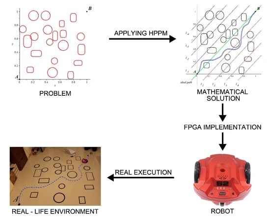
Otherwise, there are deterministic methods, that is, methods for obtaining trajectories that are executed only once with the certainty that, if the problem has at least one real solution, it will be found; one of these methods is the Homotopic Path Planning Method (HPPM) [8,28,29,30,31,32]. The HPPM makes use of the Homotopic Continuation Method (HCM), which has been initially used to solve systems of Non-linear Algebraic Equations (NAEs) for the case when these systems have multiple solutions. These are found through the conversion of a homotopic map; HPPM includes obstacle representation within the environment through mathematical singularities in the system of equations to be solved. To generate the homotopic conversion, one starts from a system of nonlinear equations with known solution values and ends when solutions of the desired system of equations are reached by integrating on an additional term known as the homotopic parameter ($\lambda$). During this conversion, a family of $\gamma$ curves is generated and within all of them, the HPPM will take advantage of the one that implicitly contains the collision-free path. In the study cases presented in this article we will only work in two dimensions; nevertheless, the HPPM algorithm can be expanded to n-dimensions, as shown in [8]. An advantage of the HPPM is, when applied in environments with a high density of obstacles and narrow corridors as well [31], memory use and computation time increases at slower rate compared to the methods previously mentioned, especially if it is considered that the solution method could be implemented in an embedded system like a Field Programmable Gate Array (FPGA). This work proposes a methodology that properly assigns the repulsion parameter for terrestrial mobile robots, given that it constitutes a key value for finding an optimized collision-free path. The goal is to obtain a solution path as close to the optimum, in terms of distance, as possible.

This paper is organized as follows: Section 2 describes HCM and the path planning solution using HPPM. Description of the repulsion parameter and proposed methodology for its assignment is described in Section 3. The implementation of this in a FPGA is presented in Section 4. Three study cases are provided in Section 5. A brief discussion is given in Section 6. Finally, Section 7 presents the conclusions of this work.

2. Homotopy Continuation Method as a Collision-Free Path Planning Method

The Homotopy Continuation Method (HCM) is used to solve NAEs applying a procedure that involves transforming the NAEs into a trivial problem simple to solve; then, it transforms gradually the trivial problem into the original NAEs increasing the probability of finding a solution. The NAEs to solve is:

$$f\left(x\right)=0,f\in {\mathbb{R}}^n⟶{\mathbb{R}}^n,$$

(1)

where n indicates the number of x variables of the problem. Based on this, a homotopic map is generated, which has the following representation:

$$H(f\left(x\right),\lambda )=0,H\in {\mathbb{R}}^{n+1}⟶{\mathbb{R}}^n,$$

(2)

where the homotopic parameter $\lambda$ is responsible for carrying out the continuous deformation of the system of NAEs during its sweep from 0 to 1. When $\lambda =0$ the solution of the system for $H^{-1}\left(0\right)$ is known or can be calculated by numerical methods in a simple way; when $\lambda =1$ the function $H\left(f\right(x),1)=f\left(x\right)$, which implies that the set of solutions for $f\left(x\right)$ has been found.

The perturbations that the homotopic system goes through generates a family of $\gamma$ curves; nevertheless, not all of these curves generate the path from $\lambda =0$ to $\lambda =1$, some produce closed curves and others tend to diverge without intersecting at $\lambda$ = 1. The curve that generates the path from $\lambda =0$ to $\lambda =1$ is what essentially constitutes the solution for trajectory analysis. A possible representation to generate the homotopic map would be:

$$H\left(f\right(x),\lambda )=\lambda f\left(x\right)+(1-\lambda )G\left(x\right)=0,\lambda \in [0,1],$$

(3)

where, $G\left(x\right)$ is a simple solving system. For this study, the method known as Newton’s homotopy [33] is used, where through $G\left(x\right)=f\left(x\right)-f\left(x_0\right)$ allows one to find solutions of the system based on an initial point $x_0$. Its representation usually looks like the following:

$$H(f\left(x\right),\lambda )=\lambda f\left(x\right)+(1-\lambda )(f\left(x\right)-f\left(x_0\right))=0.$$

(4)

During the process, the value of $\lambda$ may increase or decrease as it encounters backward trajectories; therefore, predictor-corrector scheme shall be repeated until $\lambda$ exceeds the value of 1, which means that the original system has been solved and the homotopic path that goes from $\lambda =0$ to $\lambda =1$ has been found. For all this to take place, it is important to define the system of non-linear equations appropriately; once this has been defined, a suitable numerical continuity method is proposed, otherwise global convergence of the system cannot be guaranteed.

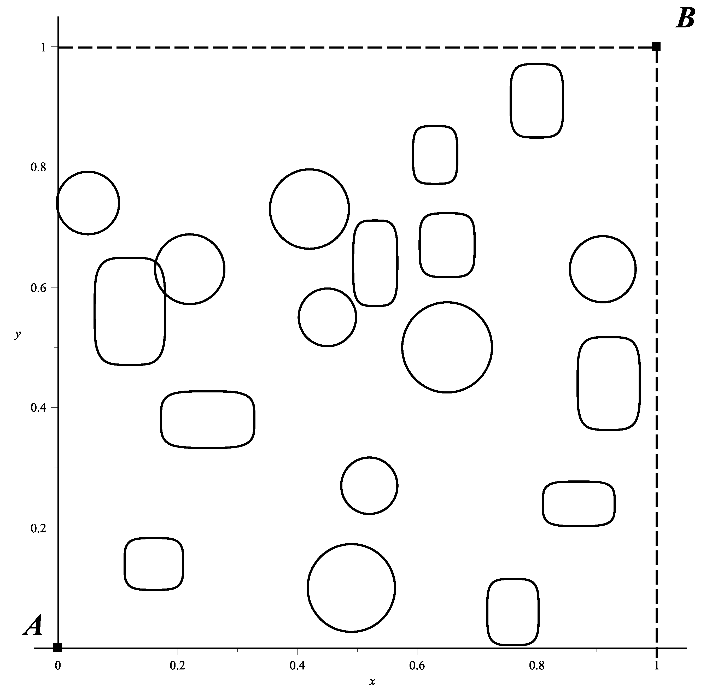
In order to solve the problem for robotic applications presented in this investigation, it is important to take into account the management of a normalized space, that is, dimensions adjustment. Then, it is considered to reduce HPPM complexity from n-dimensions to only two of them. Initial position $A=(x_{initial},y_{initial})$ is set, for this article, at $A=(0,0)$; then, goal point $B=(x_{goal},y_{goal})$ will be $B=(1,1)$, delimited by a unitary length and width map. In addition, it must be aided by a pair of equations whose only solution is found at end point $B=(x_{goal},y_{goal})=(1,1)$, so that:

$$\begin{array}{c}{f}_1(x,y)=0,x,y\in \mathbb{R},\\ f_2(x,y)=0,x,y\in \mathbb{R}.\end{array}$$

(5)

In such a way that $f_1(1,1)=0$ and $f_2(1,1)=0$. This is how a pair of linear equations can be established:   

$$\begin{array}{c}{L}_1(x,y)=ax+by+c=0,x,y\in \mathbb{R},\\ L_2(x,y)=dx+ey+f=0,x,y\in \mathbb{R},\\ m_1=-a/b,\\ m_2=-d/e,\end{array}$$

(6)

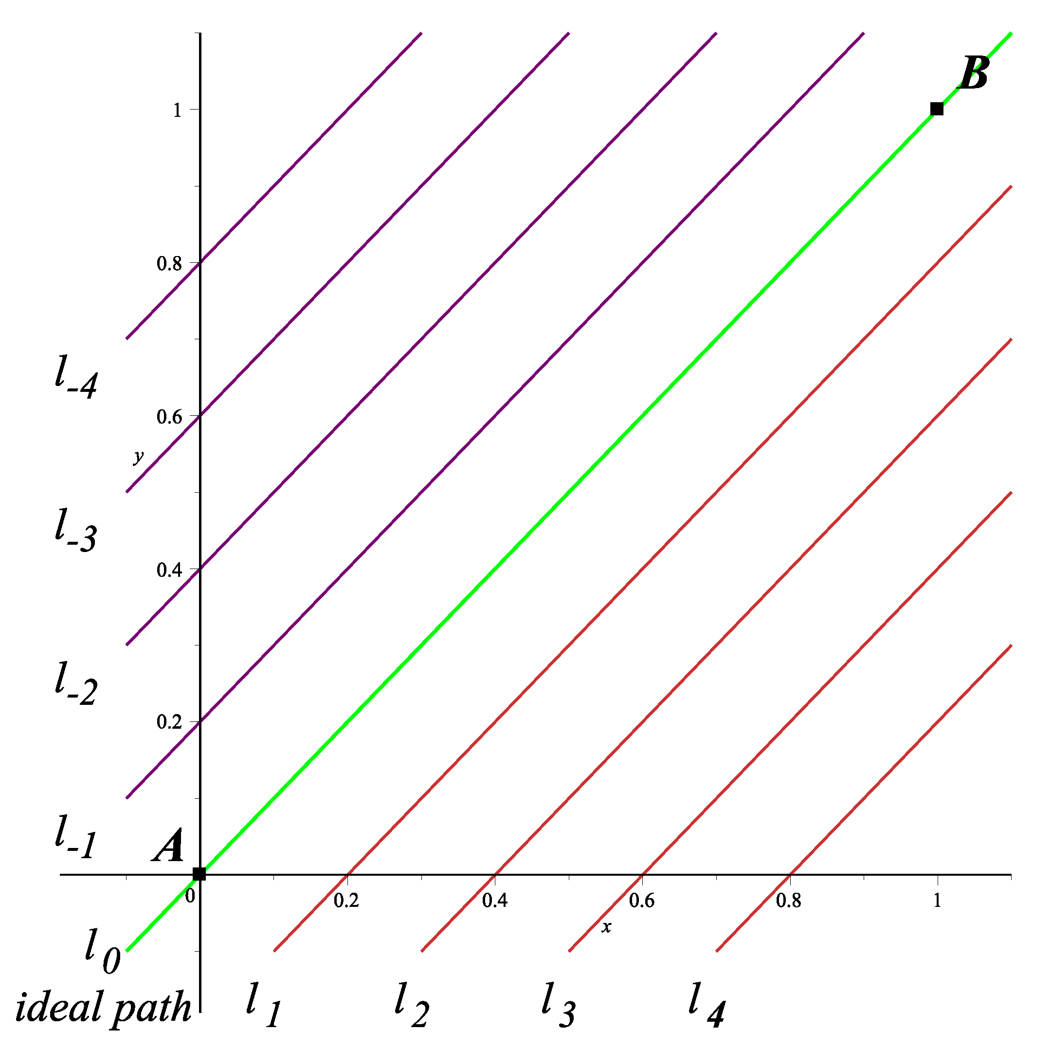
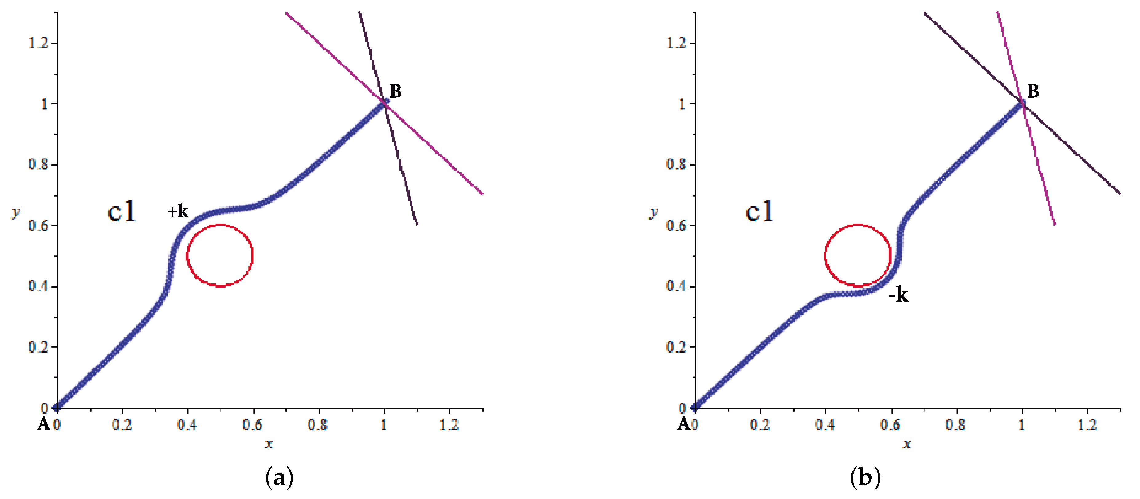
where, a, b, c, d, e and f are constants so that these lines intersect at point $B=(x_{goal},y_{goal})=(1,1)$. For this work, we propose $c=(1+m_1)$ and $f=(1+m_2)$, where, $m_1$ and $m_2$ represent the respective slopes of each auxiliary line. As already mentioned, homotopy will start from a simple, or known solution; as for this case, the one generated by the crossing of lines $L_1$ and $L_2$.

Values used here are $m_1=-4$ and $m_2=-1$, since they have shown that to accomplish the desired behavior of the resulting trajectory, according to the study carried out in [31] with various combinations of slopes for the crossing of line $L_1$ with $L_2$.

Once the standardized space has been established, obstacles must be included. HPPM can work with all kinds of obstacles represented with closed curves where, for this article, we will use circular and rectangular representations. Circular obstacles are represented as:

$$C_i(x,y)={(x-x_i)}^2+{(y-y_i)}^2-{\left(r_i\right)}^2,$$

(7)

where $(x_i,y_i)$ are the coordinates of the i-th circular obstacle of radius $r_i$. While rectangular obstacles are analytically approximated through the ellipsoidal equation:

$$R_i(x,y)={\left(\frac{x-x_i}{{\alpha }_i}\right)}^{2\eta }+{\left(\frac{y-y_i}{{\beta }_i}\right)}^{2\eta }-1,$$

(8)

where $(x_i,y_i)$ are the coordinates of the center of the i-th rectangular obstacle, and the base and height approximations approach $2\alpha$ and $2\beta$, respectively, as $\eta$ tends to infinity; for this study, $\eta =2$ defines the vertices of each rectangle. Supported by these descriptions, the set of obstacles in [31] are expressed through:

$$W(x,y)=\sum _{i=1}^k\left(\frac{p_i}{|{\mathrm{Obj}}_i(x,y)|+{\mathrm{Obj}}_i(x,y)}\right),$$

(9)

where $Ob{j}_i$ could be either, $C_i(x,y)$ or $R_i(x,y)$; $p_i$ is known as the repulsion parameter assigned to the i-th obstacle $Ob{j}_i$. To complete the inclusion of obstacles to the system, a compensation function must be generated:

$$Q=W(1,1)=\sum _{i=1}^k\left(\frac{p_i}{|{\mathrm{Obj}}_i(1,1)|+{\mathrm{Obj}}_i(1,1)}\right),$$

(10)

which evaluates the alterations caused by the obstacles at final point $B=(x_{goal},y_{goal})=(1,1)$. With this, the full system of non-linear equations can be established that will describe the problem:

$$\begin{array}{cc}{f}_1(x,y)=L_1(x,y)=0& x,y\in \mathbb{R},\\ f_2(x,y)=L_2(x,y)+W(x,y)-Q=0& x,y\in \mathbb{R},\end{array}$$

(11)

which converts the equation $f_2$ into the constraint equation. Applying (11) in (4) it gets:

$$\begin{array}{c}{H}_1(f_1(x,y),\lambda )=f_1(x,y)-(1-\lambda )f_1(x_0,y_0)=0,\\ H_2(f_2(x,y),\lambda )=f_2(x,y)-(1-\lambda )f_2(x_0,y_0)=0,\end{array}$$

(12)

where starting point A has coordinates $(x_0,y_0)$. Therefore, the system is established (see Figure 1).

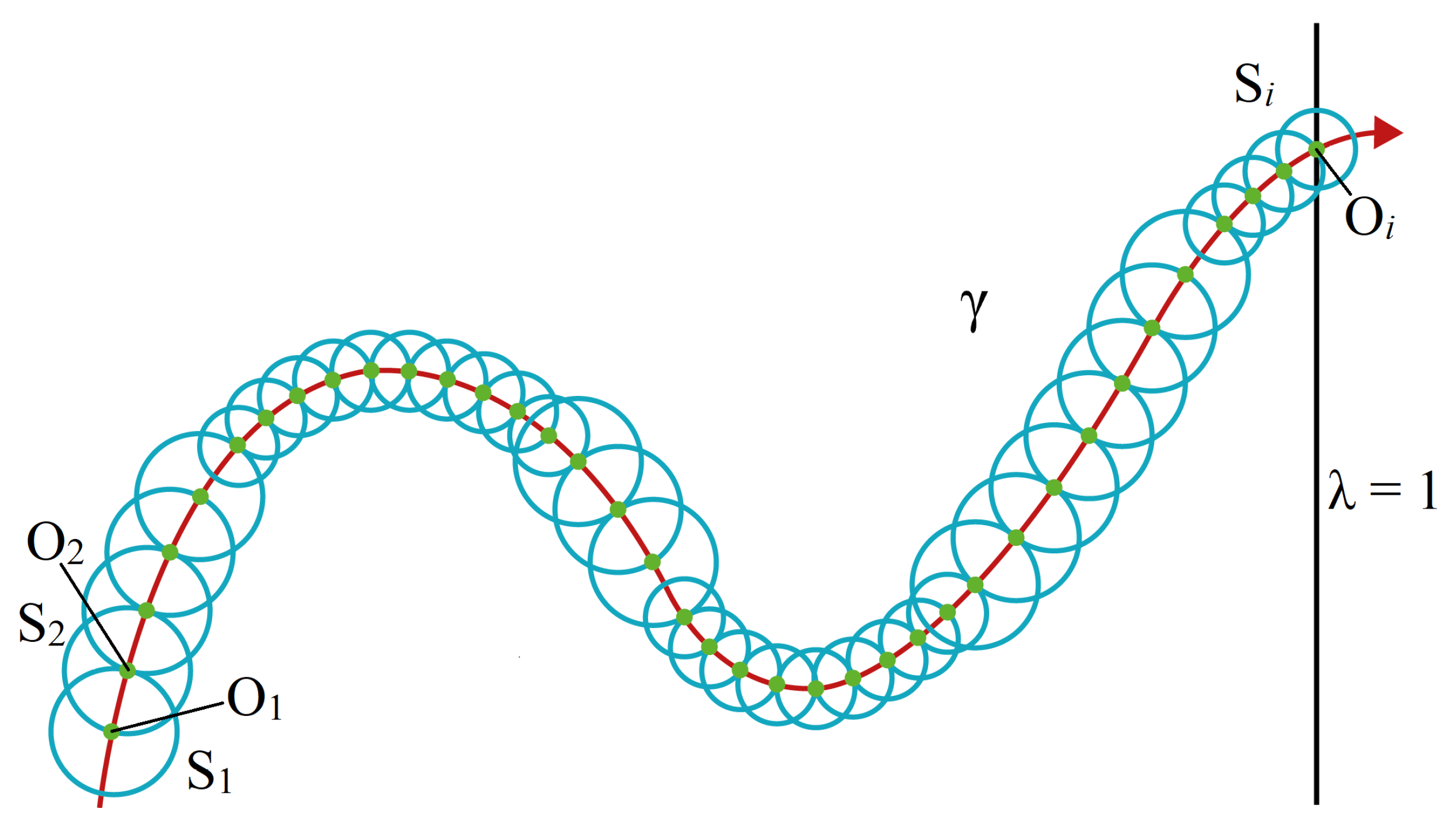
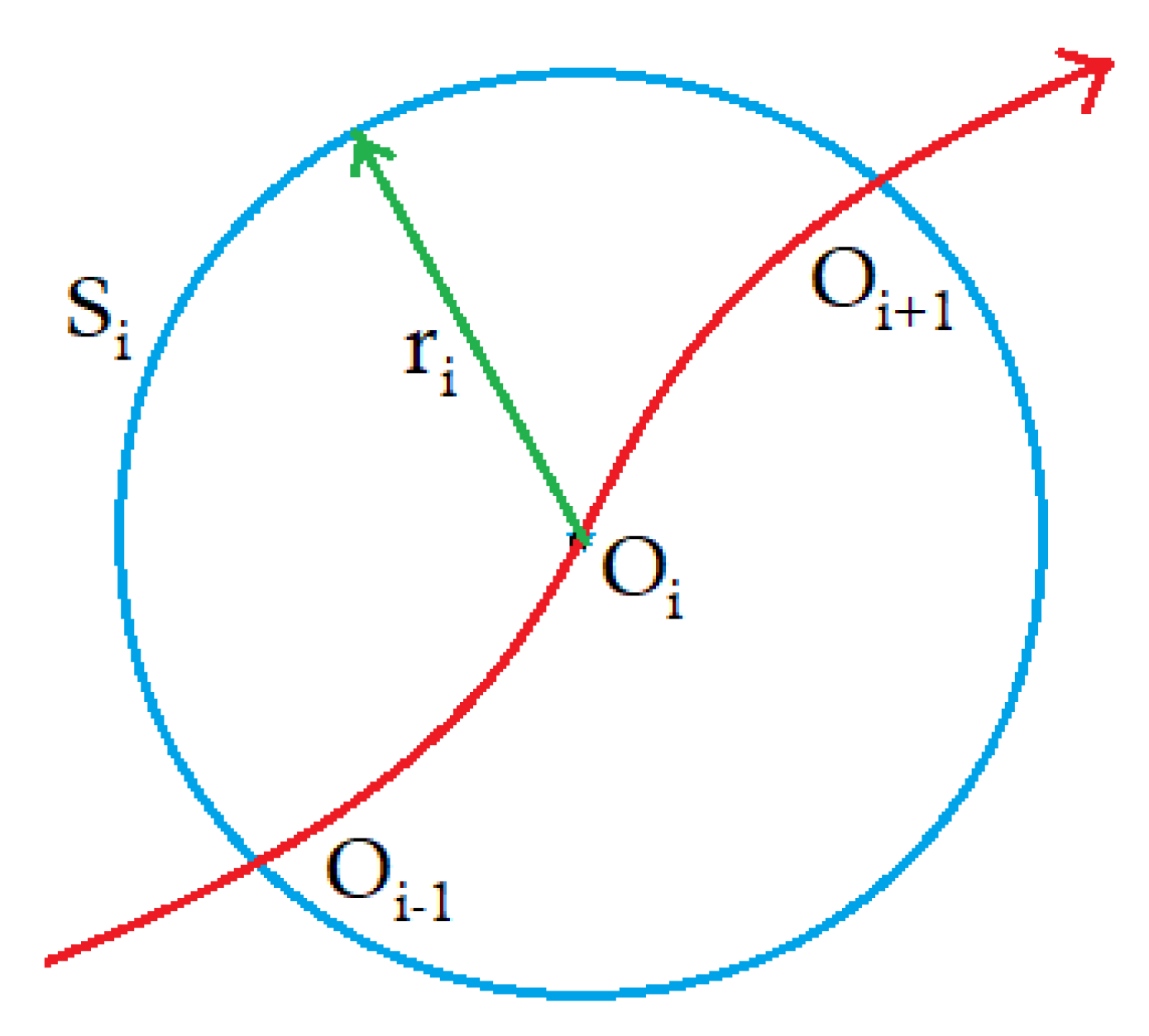
An appropriate path tracking procedure that supports HPPM should be considered. One of them is the Hyperspherical Algorithm [34,35,36] which, as its name implies, is based on the generation of an n-dimension sphere with radius r and its center lies on the homotopic curve in $O_i$. The contour of this sphere touches at least two points of the same curve, $O_{i+1}$ and $O_{i-1}$, as can be seen in Figure 2.

A terrestrial robot has two-dimension variables ($(x,y)$); in addition, there is the need to provide the homotopic parameter $\lambda$; therefore, the algorithm will use an equation dependent on three variables, represented by:

$$S_i(x,y,\lambda )={(x-c_x)}^2+{(y-c_y)}^2+{(\lambda -c_{\lambda })}^2-r_i^2=0,$$

(13)

where $(c_x,c_y,c_{\lambda })$ is the center $O_i$ of each sphere and $r_i$ its particular radius. Combining this new function with the system (12), the following system is obtained:

$$\begin{array}{c}{H}_1(f_1(x,y),\lambda )=f_1(x,y)-(1-\lambda )f_1(x_0,y_0)=0,\\ H_2(f_2(x,y),\lambda )=f_2(x,y)-(1-\lambda )f_2(x_0,y_0)=0,\\ S_i(x,y,\lambda )={(x-c_x)}^2+{(y-c_y)}^2+{(\lambda -c_{\lambda })}^2-r_i^2=0,\end{array}$$

(14)

The algorithm changes values after each iteration, that is, updates the center value; in addition, some curve segments may have very closed return points, then, radius values vary to prevent reversal of jump issues between homotopic curves [35,37]. Figure 3 shows this adjustment based on this method. To avoid complications when designing the spheres and maintaining the homotopic trajectory, the method uses a predictor-corrector model complementing the spherical tracking.

To find the next advance position on the path, the Euler predictor algorithm is applied; the reported works [34,37,38] present and verify its effectiveness. It takes advantage of the hypersphere centered at the current position within the homotopic curve $(c_x,c_y,c_{\lambda })$ and draws a tangent vector $\overrightarrow{v_p}$ on its center; when this vector propagates in space, it touches two points of the hypersphere $S_i$. From this pair of points, the closest to the advance solution direction $\gamma$ will be selected as the predictor point; this procedure is thoroughly explained in [39,40]. According to this, predictor point $(x_p,y_p,{\lambda }_p)$ formula can be expressed as:

$$(x_p,y_p,{\lambda }_p)=(c_x,c_y,c_{\lambda })+r_i∥\overrightarrow{v_p}∥,$$

(15)

The predicted point is near the solution curve; nevertheless, it is necessary to execute the corrective algorithm so that this approximation is positioned on the homotopic path. For this case, the Newton-Raphson algorithm is used [35,37]. Thus, the corrective step can be expressed as:

$$\begin{array}{c}(x_{i+1},y_{i+1},{\lambda }_{i+1})=(x_i,y_i,{\lambda }_i)-{\left[J(x_i,y_i,{\lambda }_i)\right]}^{-1}H(x_i,y_i,{\lambda }_i),\hfill \end{array}$$

(16)

where $i=0,1,2,$...; $(x_0,y_0,{\lambda }_0)=(x_p,y_p,{\lambda }_p)$, and ${\left[J(x_i,y_i,{\lambda }_i)\right]}^{-1}$ is the inverse Jacobian matrix of $H(x_i,y_i,{\lambda }_i)$. That is the system representation at current point $(x_i,y_i,{\lambda }_i)$. Since it is an iterative method, the obtained value becomes the current value for the next iteration, and so on until any of the following situations is reached: it converges to a point in the homotopic curve, reaches a convergence value with a minimum difference established between one iteration and the next (which for this investigation has a value of $1\times {10}^{-8}$), or consumes the maximum number of iterations (50 for this procedure).

From now on, the predictor-corrector scheme, in conjunction with the hyperspheric advance scheme, will be repeated for every position progressed over the path until $\lambda$ has crossed the 1 value; which implies that there is a path from the start to goal position [8,28,29,30,31,33].

The fundamental difference from the original HPPM is that this proposal adds an automated calculation algorithm for the repulsion parameters, useful for the most complex study cases, where calculations by hand would be time-consuming and cumbersome, as can be noticed in the cases found in [31].

3. Automatic Assignment of the Repulsion Parameter

In HPPM, obstacles are considered as elements that interfere with the ideal path [8]; the repulsion parameter is a value that determines trajectory direction. It sets up a direct relation between direction and proximity distance with respect to the obstacle in such a way that, if the parameter is small, the path will be close to the obstacle. Therefore, as the parameter value increases, the path is repulsed away from the obstacle. At this point, assignment of repulsion parameters depends on the user empiric knowledge, that is, based on previous experiences. Recently, an alternative of automatic assignation to the repulsion parameter in the homotopic method has been provided [30], which is explained below.

3.1. Assignment of the Repulsion Parameter

To assign the repulsion parameter, it is necessary to know the initial point (A) and goal position (B); then, we can define an ideal path, represented by a straight line, between these two points ($l_0$). In addition, we define a set of auxiliary straight lines which are parallel and equidistant to the ideal path. These paths are defined as

$$l_i:y-y_i=m(x-x_i),$$

(17)

where i takes integer values, positive or negative, depending on the required regions in the solution space. To establish this, qualitative tests were carried out modifying the number of auxiliary lines and obstacles quantity. For the cases of one and two auxiliary lines (Figure 4a), the influence of these lines on the behavior of obstacles is minimal. In addition, if obstacle number increases, this influence practically disappears.

For three auxiliary lines (Figure 4b), the regions influence associated to these lines can be perceived and the strength of the repulsion parameters begins to numerically reinforce the idea of maintaining calculated trajectory close to the ideal path. Nevertheless, since each obstacle is compared in position to every auxiliary line, the execution time importance of this algorithm also begins to be noticed.

For the case of four auxiliary lines (Figure 4c), the regions influence improves according to the repulsion parameter settings; for this option, execution time becomes considerable, especially if the amount of obstacles increases.

Tests were carried out with five auxiliary lines and more (Figure 4d–f). As a result, regions influence on repulsion parameters remains effective, although the time required for the algorithm to assign values after the sweep of positions for each obstacle with respect to the auxiliary trajectories exceeds the main algorithm’s execution time.

Furthermore, noticing that the improvement ratio between the number of auxiliary lines and the resulting path is linear, while the relationship between the assignment of repulsion parameters algorithm execution time and the number of obstacles grows exponentially, we found that four auxiliary lines per side is the best option.

These auxiliary straight lines (17) are employed to compare every obstacle position with respect to the ideal path (green line in Figure 5), in such way that if the obstacle is close to this ideal path, the algorithm will assign a relatively small repulsion value causing the obtained trajectory to stay close to the mentioned ideal path; if the obstacle is far from the ideal path, a higher repulsion value will be assigned, keeping the trajectory away from the area where the mentioned obstacle is and adjusting the trajectory closer to the ideal path.

This turns (17) into (18), such that:

$$l_i=l_k:y-y_k=m(x-x_k)\Rightarrow (k\in \mathbb{R}\mid k=[-4,4];k\ne 0);$$

(18)

where i turns into k; k takes integer values ranging from $-4$ (for obstacles above the ideal path) to 4 (for obstacles below the ideal path). Taking this into account, when $i=0$, this represents the value of the ideal path (Figure 5).

The k values are important when establishing repulsion parameter sign, since, as stated in the formula, these k values are accompanied by a sign. Repulsion parameter sign defines if trajectory will pass above or below the obstacle; it is defined that obstacles above the ideal trajectory are assigned a negative repulsion parameter value (k from −1 to −4 in (18)) forcing the path to continue below these obstacles. Reciprocally, if those are below the ideal route, a positive repulsion parameter value will be assigned (k from 1 to 4 in (18)) causing the path to pass above these obstacles. For both cases, the purpose is to calculate a trajectory that approaches the ideal path as much as possible (see Figure 6).

Then, initial minimum values are established for different obstacles. Circular obstacles predetermined value $p_{0c}$ is set to $0.0001$. As for rectangular obstacles, $p_{0r}$ value is $0.1$. These values have been obtained in heuristic form, analyzing different paths and obstacle quantities and therefore are defined as the optima for automatic assignment. This is described as

$$\begin{array}{c}\hfill p_{i,c}=k·p_{0c},\\ \hfill p_{i,r}=k·p_{0r},\end{array}$$

(19)

where i indicates the number of obstacles and k is the weight associated to the auxiliary line closest to the obstacle, as already explained.

3.2. Obstacle Grouping by Vicinity

Due to the proximity between obstacles, repulsion parameters may cause conflicts on the path; this may lead to finishing at indefinite trajectories or dead-ends (Figure 7a,b). Therefore, it is necessary to group sets of contiguous or close obstacles that the path may encounter or pass nearby to try to avoid these problems.

The way to determine how obstacles can be considered a problem is through the comparison of two distances; the first, distance between centers

$${\mathrm{dc}}_{ij}=\sqrt{{(x_i-x_j)}^2+{(y_i-y_j)}^2},$$

(20)

where position ($x_i$,$y_i$) is the center of the i-th obstacle and point ($x_j$,$y_j$) is the center of the j-th obstacle. The second distance to compare relates to the minimum required distance for the robot to cross between two obstacles, any value below the set requirement will be considered as an obstructing object; it is obtained by

$${\mathrm{di}}_{ij}=g·d_r+\max (r_i,h_i)+\max (r_j,h_j),$$

(21)

where $d_r$ is the diameter of the robot; $g=1.1$ is an empirical parameter that represents a safety radius of 10% of the robot size, thus avoiding collisions, especially when sharp turning points are found; $r_i$ is the radius of the i-th obstacle for circular; $h_i$ is the hypotenuse resulting from analyzing the baseline $\left(2\alpha \right)$ and height $\left(2\beta \right)$ values of rectangular obstacles, and max is a function that determines the biggest value between $r_i$ and $h_i$, and between $r_j$ and $h_j$.

If distance between centers (20) of a pair of $ij$ obstacles is less than the obstruction distance (21), it is said that a ”neighbourhood” exists between them and an adjustment of their repulsion parameters should be considered because it is not possible to pass between them if the path planning requires it. This concept is explained in the next subsection.

3.3. Correction of the Repulsion Parameter

Once neighbourhoods are defined, the next step in this methodology is to standardize the sign of all obstacles found in each neighbourhood to avoid a dead-end.

Correction of the repulsion parameter allows one to consider the set of obstacles within the neighbourhood as one big object; thus, the resulting path will surround it on one side or the other depending on the nearest group sign. The sign is obtained by an iterative comparison of all the obstacles grouped in each neighbourhood, setting the obstacle sign with the largest area within the vicinity. If all obstacles have the same dimensions, the sign is set randomly.

As can be seen in Figure 8a, there is a neighbourhood with sign conflict; obstacles located above the ideal trajectory show a negative repulsion parameter while obstacles located below the ideal trajectory have a positive repulsion parameter assigned to them. In order to avoid a path planning issue, the obstacle with the largest area provides its sign (positive or negative) as the dominant sign of the neighbourhood; this means that every obstacle within this neighbourhood has the same sign; forcing the path planning method to surround them all as if they were a single obstacle (Figure 8b).

4. FPGA Implementation

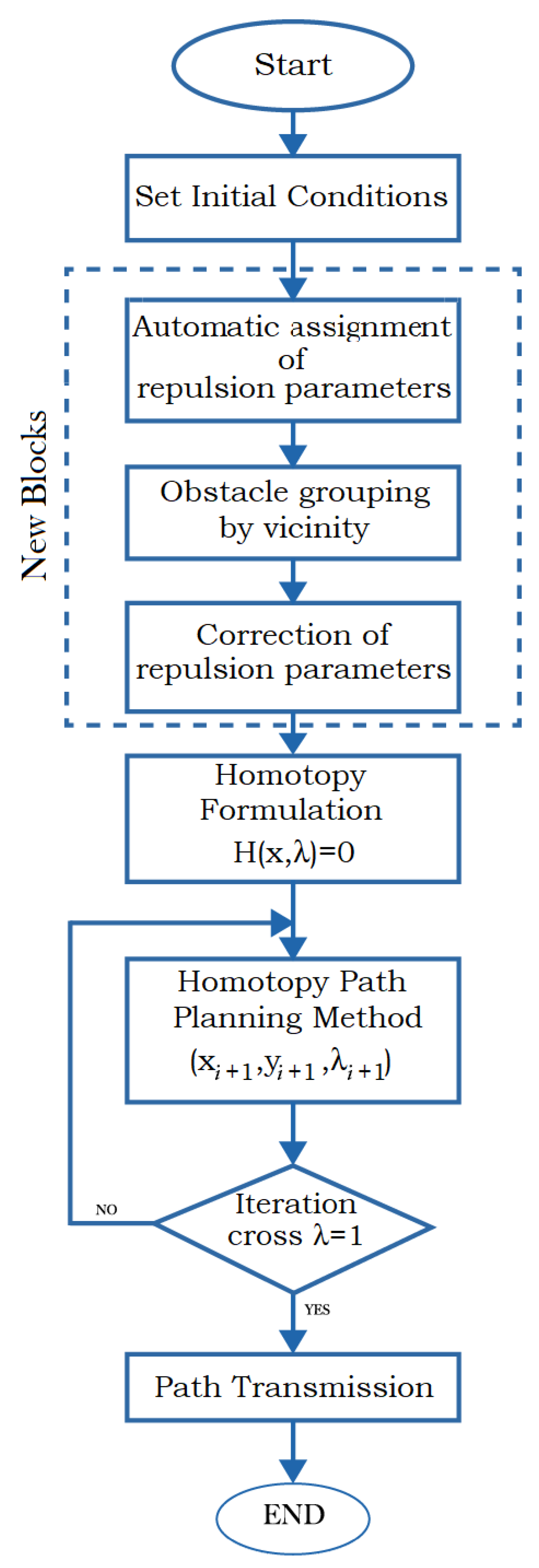
The FPGA implementation in this work, and other implementations on PC or embedded devices [31], is designed to allow the user to select different initial and goal points within the normalized space (that is, between 0 and 1) and also to modify the quantity and position of obstacles present in this normalized space. Algorithm 1 presents the general algorithm programmed in the FPGA.

Algorithm 1 General algorithm

1: procedureGeneral($x,y,\lambda$) 2:         Set initial conditions 3:         Automatic assignment of repulsion parameters 4:         Obstacle grouping by vicinity 5:         Correction of repulsion parameters 6:         Homotopy formulation 7:         Homotopy Path Planning Method 8:         if $\lambda <1$then                                                                                ▹ Stop path tracking condition 9:                Return to Homotopy Path Planning Method 10:         end if 11:         Path transmission 12: end procedure

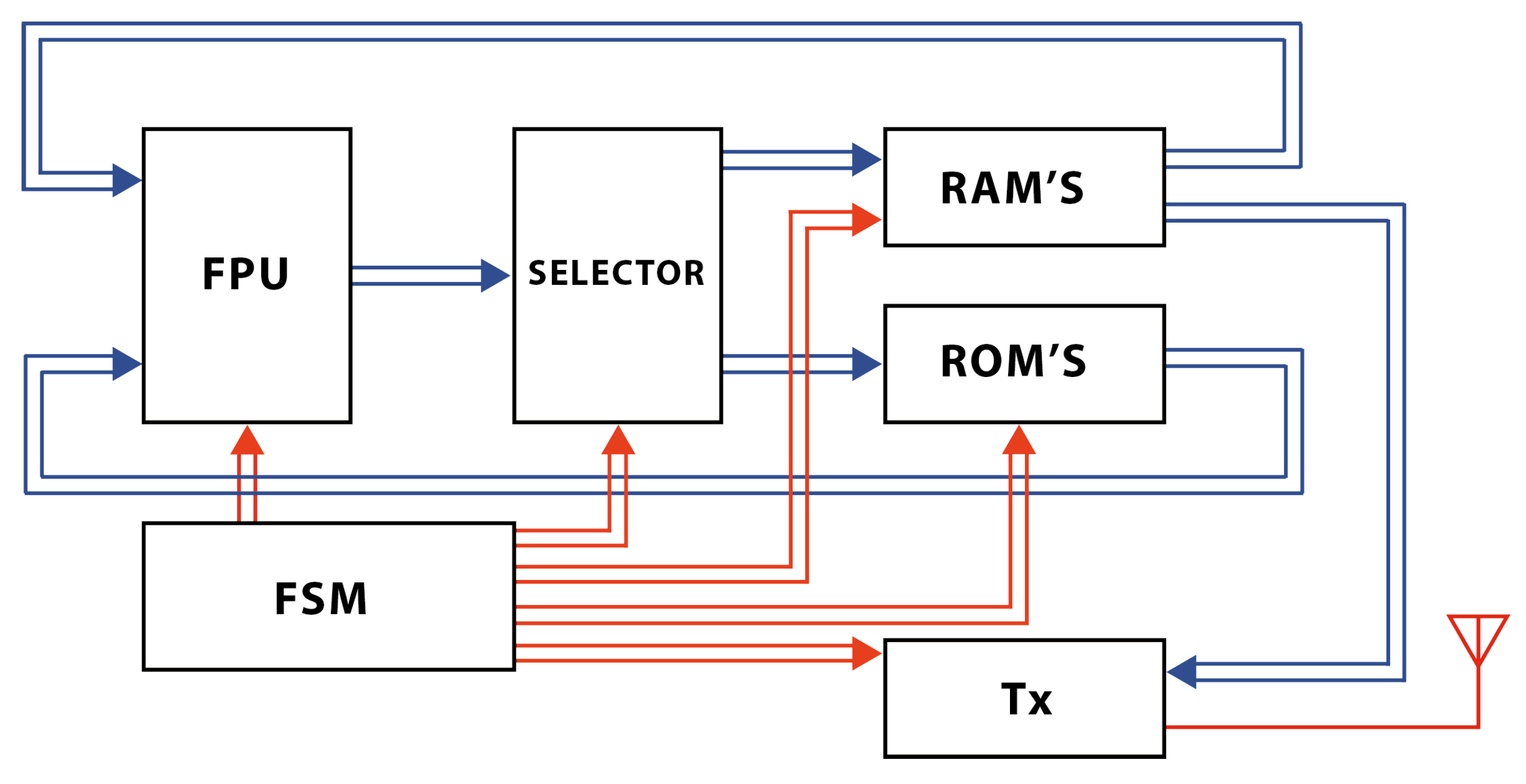
The implemented program in the FPGA consists of an arithmetic floating-point unit (FPU), a set of ROM memories that store obstacle position data, a set of RAM memories to store intermediate results of calculations from the homotopic system, and the $(x,y)$ values of the resulting homotopic path; all these elements are controlled using a finite state machine (FSM) that synchronizes the application of every methodology step described in this work (Figure 9).

At the first stage of the program (Algorithm 2), obstacles present in the environment have to be declared, as well as some other parameters needed by the homotopic simulation (step size, error criterion, among others). FSM coordinates the sequence in which routines will be executed and provides memory management. It is important to note that the dotted-line box in Figure 10 encloses the three new blocks (algorithms) proposed in this work. The rest of the diagram belongs to the original HPPM algorithm [8].

Algorithm 2 Initial conditions

1: procedureSet initial conditions($x,y,\lambda$) 2:        RAM ← initial ($x_i,y_i,{\lambda }_i=0$) and final position ($x_f,y_f,{\lambda }_f=1$) 3:        Set number and position of $C_n$ and $R_n$ obstacles                                          ▹ Stored at ROM 4:        RAM ← stablish hyperspherical standard size 5: end procedure

When the automatic assignment of repulsion parameter starts (Algorithm 3), a comparative cycle is established between every obstacle center and the auxiliary straight lines ($l_i$). To accomplish this, the state machine sends, one by one, the address corresponding to the center of every obstacle from the ROM memories; the data from these locations are compared to the auxiliary straight lines (17) and the resulting values are stored in RAM at specific locations addressed from the FSM.

Algorithm 3 Assignment of repulsion parameters

1: procedureAutomatic assignment of repulsion parameters($p_i$, finish1) 2:        RAM ← Calculate slope with initial and final position 3:        RAM ← Set auxiliary lines for assignment of repulsion parameters ($l_{-4}\dots l_4$) 4:        for i = 1 to number of obstacles do 5:               RAM ← Calculate distance between i-obstacle and each auxiliary line 6:               case distance is 7:                   when closer to $l_{-4}\Rightarrow p_i=-4\ast p_0$                             ▹$p_i$ is $i-$obstacle repulsion parameter 8:                   when closer to $l_{-3}\Rightarrow p_i=-3\ast p_0$ 9:                   when closer to $l_{-2}\Rightarrow p_i=-2\ast p_0$ 10:                 when closer to $l_{-1}\Rightarrow p_i=-p_0$ 11:                 when closer to $l_1\Rightarrow p_i=p_0$ 12:                 when closer to $l_2\Rightarrow p_i=2\ast p_0$ 13:                 when closer to $l_3\Rightarrow p_i=3\ast p_0$ 14:                 when others $\Rightarrow p_i=4\ast p_0$ 15:            end case 16:            RAM $\leftarrow p_i$ 17:        end for 18:        set flag finish1 on 19: end procedure

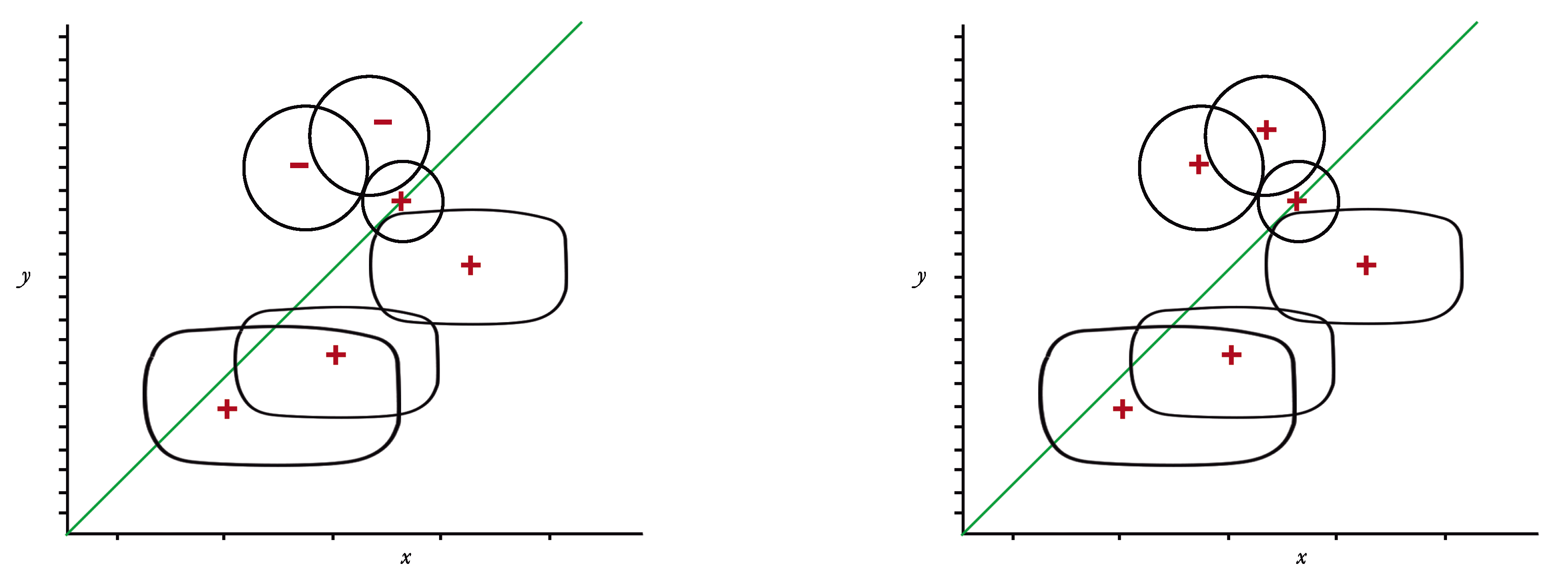
Once the repulsion parameters have been determined for all obstacles, neighbourhoods are analyzed (Algorithm 4) calculating distances between obstacles and generating indicators that find contiguous or overlapping elements that may cause issues when calculating the resulting trajectory. Similarly, the state machine will indicate sequences, addresses, modules, and operations to be employed when grouping obstacles by vicinity. In case of detecting neighboring obstacles, it adjusts the group repulsion parameter with the sign of the largest obstacle prevailing (Algorithm 5).

Algorithm 4 Obstacle grouping

1: procedureObstacle grouping by vicinity(finish2) 2:        Read robot security radius from ROM 3:        for i = 1 to number of obstacles do 4:              RAM ← Calculate space between i-obstacle and i+1-obstacle 5:              if space between obstacles < robot security radius then 6:                    obstacle vicinity marker on 7:                    RAM ← vicinity takes i+1-obstacle number as i-group number 8:              else 9:                    obstacle vicinity marker off 10:                    end if 11:          end for 12:          set flag finish2 on 13: end procedure

Algorithm 5 Correction of repulsion parameters

1: procedureCorrection of repulsion parameters(finish3) 2:        for i = 1 to number of obstacles do 3:              if i-obstacle number = i-group number then 4:                     RAM $\leftarrow p_i$ keeps original value                      ▹$p_i$ is $i-$obstacle repulsion parameter 5:             else 6:                     $p_i$ sign = i-group number sign 7:              end if 8:        end for 9:        set flag finish3 on 10: end procedure

The next set of states establishes the system homotopic equations to be solved (Algorithm 6); the representative functions already include the obstacles present in the environment (14). Once this system is obtained, the hyperspherical path tracking process begins; obtaining the resulting path as a collection of points and storing them in RAM (Algorithm 7). Once the entire path is established, data transmission to the robot begins.

Algorithm 6 Homotopy formulation

1: procedureHomotopy formulation(Homotopy equations) 2:         Set auxiliary goal position lines 3:         Call repulsion parameter values from RAM 4:         Set obstacles equations 5:         Set Newton Homotopy equations 6:         Set Jacobian equations 7:         Evaluate previous equations at initial position 8: end procedure

Algorithm 7 Homotopy Path Planning Method

1: procedureHomotopy Path Planning Method($x_i,y_i,{\lambda }_i$) 2:         for $i=1$ to maximum advance steps number do 3:               RAM ← Adjust variable radius in hypersphere calculation 4:               RAM ← Calculate Euler’s predictor position ($x_p,y_p,{\lambda }_p$) in FSM 5:               Call Euler’s predictor position form RAM and evaluate Homotopy System 6:               $x_i,y_i,{\lambda }_i\leftarrow$ Euler’s predictor position ($x_p,y_p,{\lambda }_p$) 7:               for $j=1$ to maximum iterations do 8:                     RAM ← Calculate Newton-Raphson’s corrector position ($x_c,y_c,{\lambda }_c$) in FSM 9:                     if $x_c,y_c,{\lambda }_c$ satisfies Homotopy System then 10:                           break 11:                    else if $x_c,y_c,{\lambda }_c$ approximates Homotopy System below permissible error then 12:                           break 13:                     else 14:                            Call Newton - Raphson’s corrector position form RAM and evaluate Homotopy System 15:                            $x_j,y_j,{\lambda }_j\leftarrow$ Newton-Raphson’s corrector position ($x_c,y_c,{\lambda }_c$) 16:                     end if 17:               end for 18:               $x_{i+1},y_{i+1},{\lambda }_{i+1}\leftarrow x_j,y_j,{\lambda }_j$ 19:               if ${\lambda }_{i+1}\ge 1$ then 20:                     break 21:               end if 22:        end for 23: end procedure

The FPU (SoftFloat reported in [41,42]) module is a free-code 32-bit floating-point arithmetic unit applied to this design because it requires a reduced number of cycles for the arithmetic operations. In addition, the Selector module is a set of switching units that, according to the options established by the state machine, defines whether the data to be sent to the FPU unit comes from a specific RAM or ROM and indicates the storage location of all data obtained from the FPU unit. RAM memory module allows storing results obtained from assignment of repulsion parameters and homotopic path method operations, resulting points of the homotopic path $(x,y)$, and the data conversion for the transmission of results. Otherwise, the ROM memory module stores the obstacle position data, diameters, height, and width. The transmission module $\left(\mathrm{Tx}\right)$ is an 8-bit serial transmission module that allows the communication with the robot, for this work, the Parallax’s Scribbler 2.

5. Study Cases

To show the performance of the proposed methodology (HPPM), implemented in PC and FPGA, it is compared to the sampling-based path planning algorithms EST, KPIECE, PRM (including its modification PRM Star), and RRT (including its modifications RRT Star and RRT Connect); it is also compared to the low DoF planners: Bug algorithm and the APF method.

In the following cases, all methodologies are implemented in PC attempting a fair comparison between them. The sampling-based methods were executed from an OMPL tool [43,44], which allowed us to perform a statistical analysis. The low DoF algorithms were executed using MATLAB Robotics System Toolbox since the OMPL tool does not have the designs of these algorithms.

Table 1. PC and FPGA specifications.

	PC	FPGA
	Processor	Intel Cyclone X
	Intel core i5 7300HQ	10L025
Core/Threads per core	4/1	—
Total Cores	4	—
RAM Memory	16 GB	0.594 MB (M9K)
Logic Elements (LEs)	—	25,000
DSP Blocks (18 × 18 multipliers)	—	66
Clock Speed	2.5 GHz	133 MHz
Typical Power Consumption	27.34 W	10 W
Maximum Power Consumption	45 W	15W

provides technical specifications of the hardware where all processes were run.

Nevertheless, to guarantee the results obtained from these tools are as similar as possible, all are bounded to the same conditions: for sampling-based algorithms, the searching method step size is the same as the HPPM hyperspheres; in addition, the same grid size is used for the low DoF algorithms. In the same way, all algorithms are working under the condition of movement in two dimensions only.

It is known that each methodology has certain advantages and complications according to the type of environment where it is implemented; the intention of this study is to deploy them in environments that have some conditions, both favorable and unfavorable, and thus contrast results to the proposed methodology.

All the methods on PC were implemented with 64-bit word width calculations. FPGA implementation was executed with a 32-bit word width, this due to the use of the Floating Point Unit Core [41] and certainty that the difference between results obtained in PC and FPGA are insignificant, as demonstrated in [45].

It is important to note that there is a big difference between the capabilities of a PC against an FPGA; a PC has 26,936 times more memory, its speed is 18.79 times faster, and it also consumes 2.73 times more power than an FPGA. Nevertheless, as it can be appreciated for the presentation of this study, the implementation in FPGA is highly competitive in terms of performance (memory, speed, and distance).

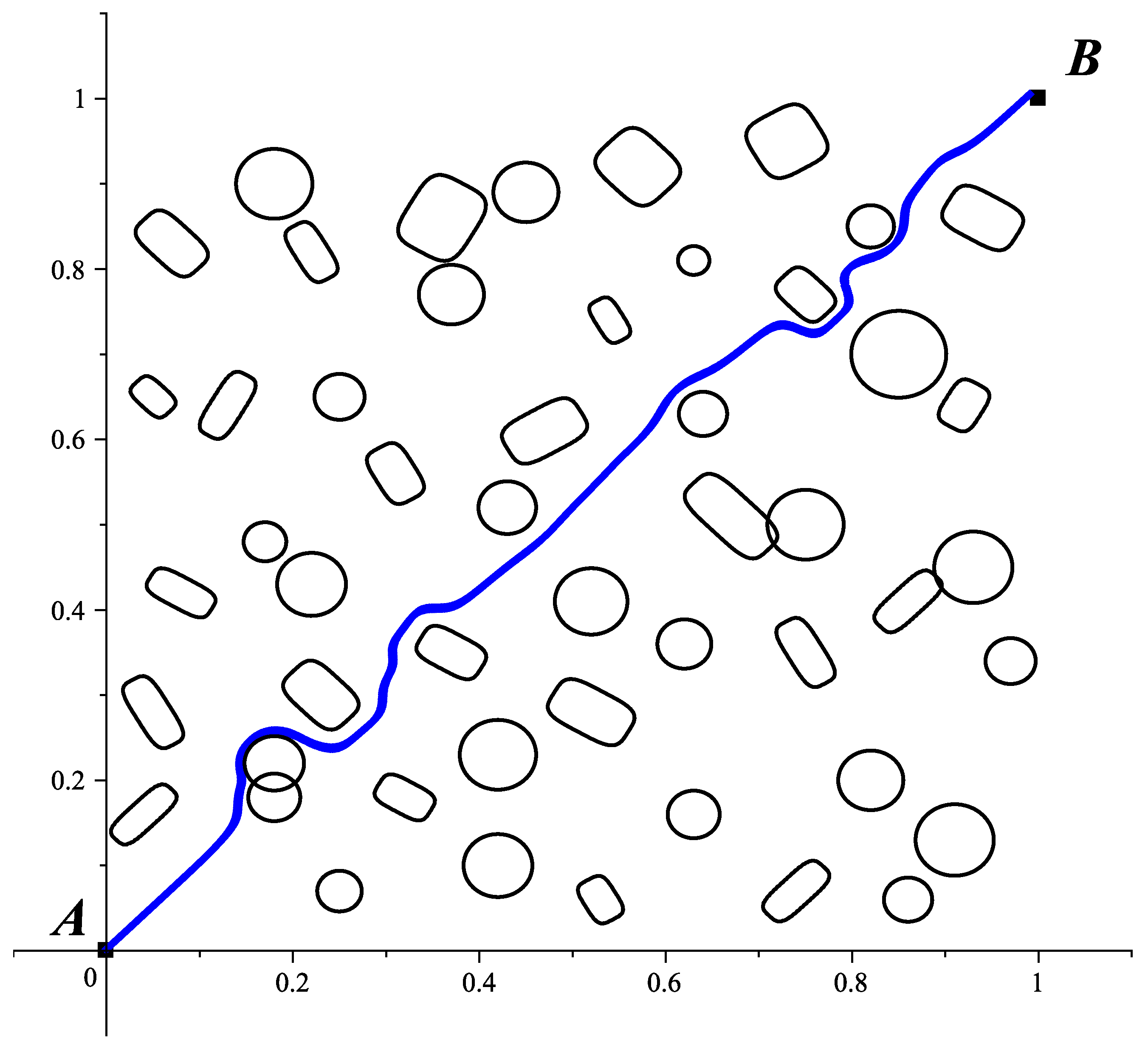
5.1. Case 1

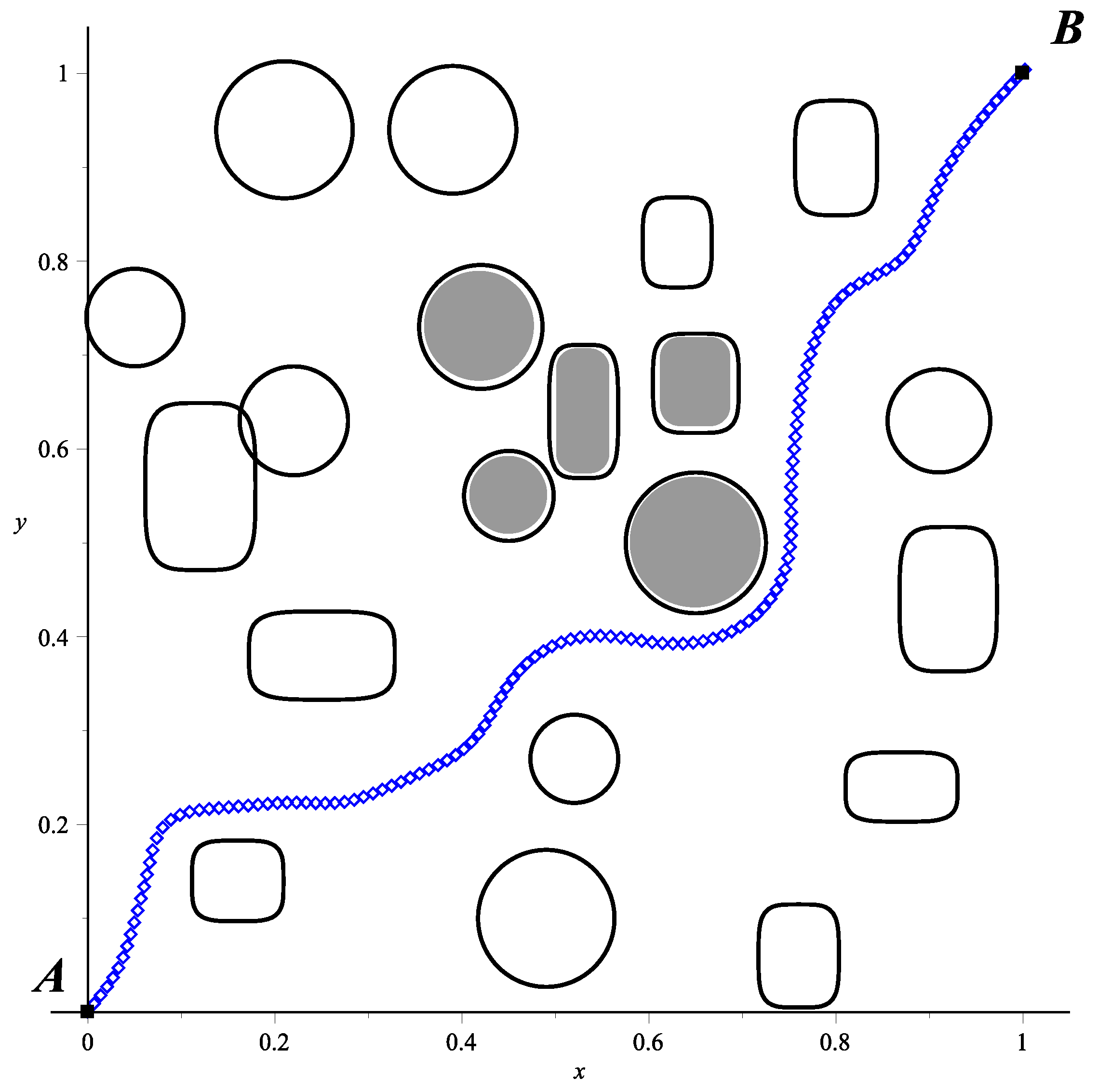
As a didactic example, an environment is generated containing 20 randomly placed obstacles. In the first instance, the development of HPPM algorithm will be presented in detail; later, results will be obtained by its implementation in the FPGA, to finally show results comparison between the HPPM and other path planning methods. It is worth mentioning that all the sampling-based algorithms were run 100 times, while the BUG, APF, and HPPM algorithms were run only once; this is because, like all deterministic methods, they will always provide the same result no matter how many times they are executed.

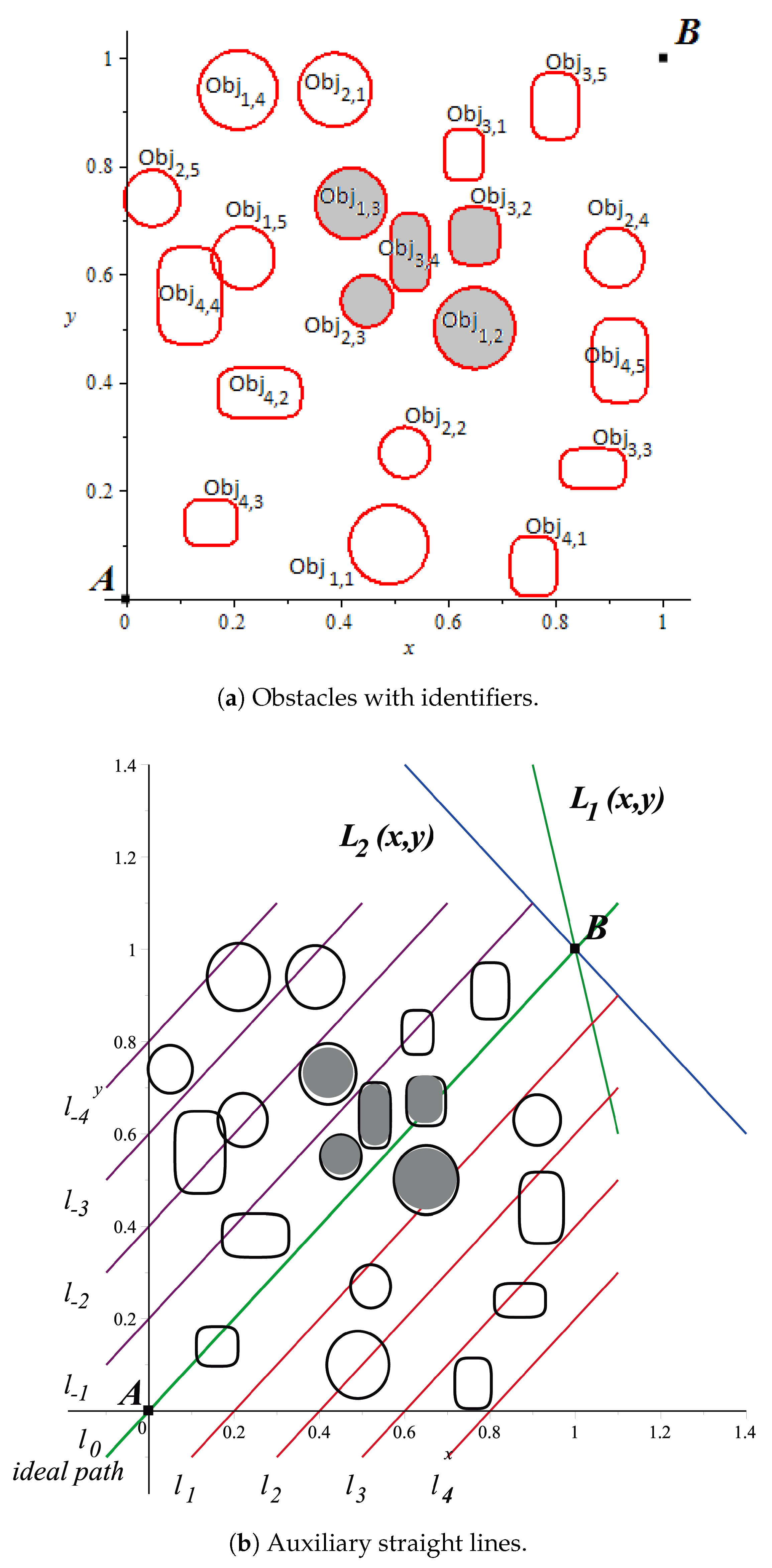
Once initial position $A=(x_{initial},y_{initial})=(0,0)$ and target position $B=(x_{goal},y_{goal})=(1,1)$ are set, obstacles are enumerated (Figure 11a). Afterwards, auxiliary straight lines (17) are generated to define the repulsion parameter (Figure 11b). As can be seen for this case, circular obstacles ${\mathrm{Obj}}_{1,2}$, ${\mathrm{Obj}}_{1,3}$, and ${\mathrm{Obj}}_{2,3}$ along with the rectangular obstacles ${\mathrm{Obj}}_{3,2}$ and ${\mathrm{Obj}}_{3,4}$ are in a vicinity; this shaded neighbourhood will be surrounded by the resulting path as a consequence of detecting this grouping and correcting the group repulsion parameter.

In

Table 2. Automatic Assignment of Repulsion Parameters.

Repulsion Parameters for Circular
and Rectangular Obstacles (${\mathbf{Obj}}_{\mathit{i},\mathit{j}}$)
	$\mathit{j}$ = 1	$\mathit{j}$ = 2	$\mathit{j}$ = 3	$\mathit{j}$ = 4	$\mathit{j}$ = 5
i = 1	0.0006	0.0002	−0.0004	−0.0008	−0.0004
i = 2	−0.0006	0.0004	−0.0002	0.0004	−0.0008
i = 3	−0.2	0.2	0.8	−0.2	−0.2
i = 4	0.8	−0.2	0.2	−0.4	0.6

the calculated repulsion parameters using (19) are shown. Next, by applying the algorithm of obstacles grouping by vicinity, some repulsion parameters are updated resulting in

Table 3. Correction of Repulsion Parameters.

Repulsion Parameters for Circular
and Rectangular Obstacles (${\mathbf{Obj}}_{\mathit{i},\mathit{j}}$)
	$\mathit{j}$ = 1	$\mathit{j}$ = 2	$\mathit{j}$ = 3	$\mathit{j}$ = 4	$\mathit{j}$ = 5
i = 1	0.0006	−0.0002 *	−0.0004	−0.0008	−0.0004
i = 2	−0.0006	0.0004	−0.0002	0.0004	−0.0008
i = 3	−0.2	0.2	0.8	−0.2	−0.2
i = 4	0.8	−0.2	0.2	−0.4	0.6

* Repulsion Parameter corrected by vicinity.

.

It is important to note that repulsion parameter of obstacle ${\mathrm{Obj}}_{1,2}$ (marked with an asterisk in Table 3) has changed because is closer to obstacles ${\mathrm{Obj}}_{1,3}$, ${\mathrm{Obj}}_{2,3}$, ${\mathrm{Obj}}_{3,2}$, and ${\mathrm{Obj}}_{3,4}$, definitive parameters used in the HPPM are those obtained in Table 3. Notice that (20) and (21) generate the neighbourhood through signs homogenization within the group, guaranteeing the adequate performance of the system during homotopic path calculation. Continuing the HPPM process execution, as expected, the homotopic path crossed below the group of gray-shaded neighboring obstacles in Figure 12.

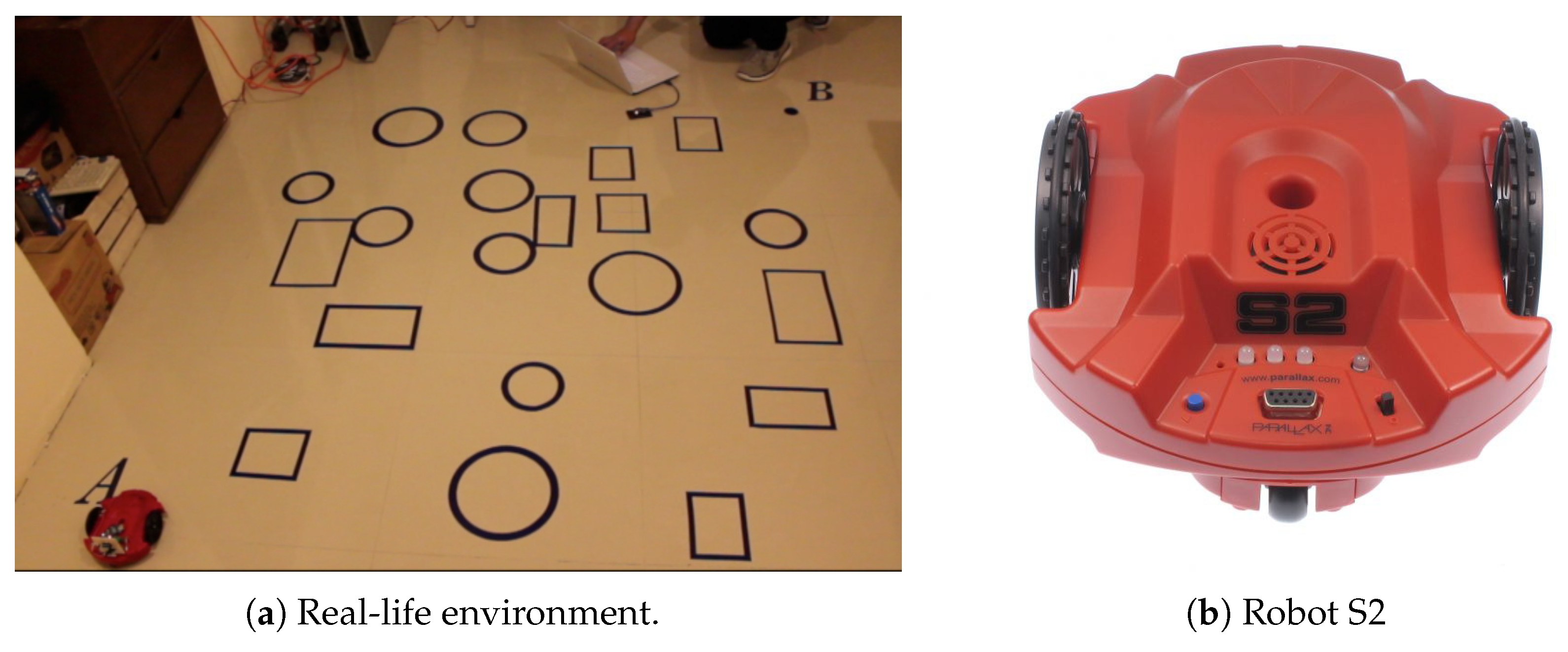
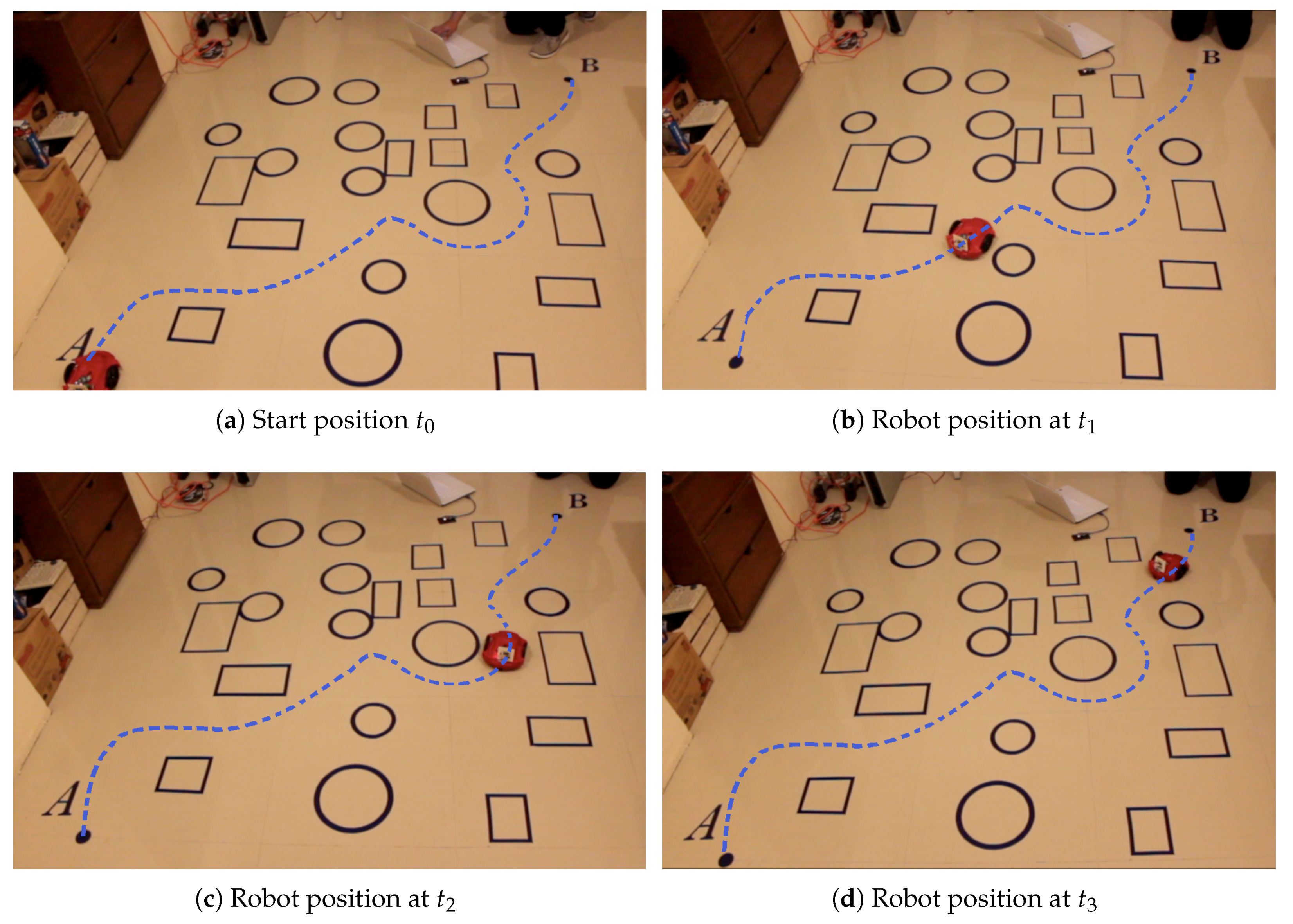
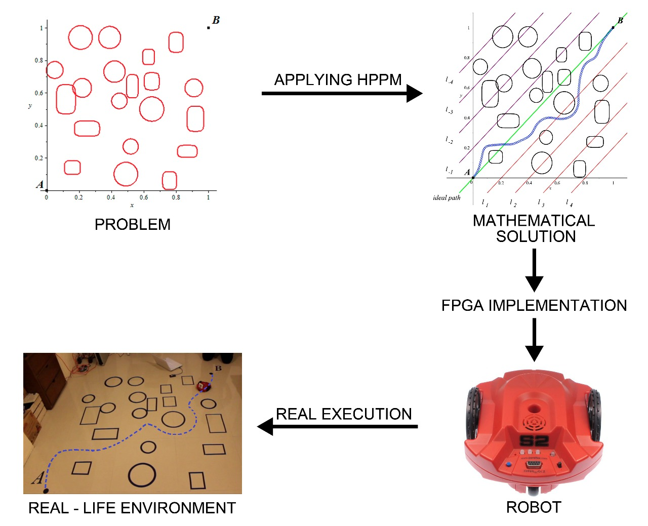
In order to show the use of our implementation in FPGA, the obtained trajectory in Figure 12 was transferred to a physical experiment (Figure 13a) testing the path calculated by the HPPM, which is provided to the Scribbler 2 robot (Figure 13b).

Information transmission to the robot is performed using an XBee 2 mW Wire Antenna device. Data transfer speed and coordinates reception by the robot are set using the Propeller Tool software. Figure 14 shows the real-life environment execution of the proposed methodology. The simulation was divided into four frames: $t_0$, $t_1$, $t_2$, and $t_3$; showing the path followed by the robot.

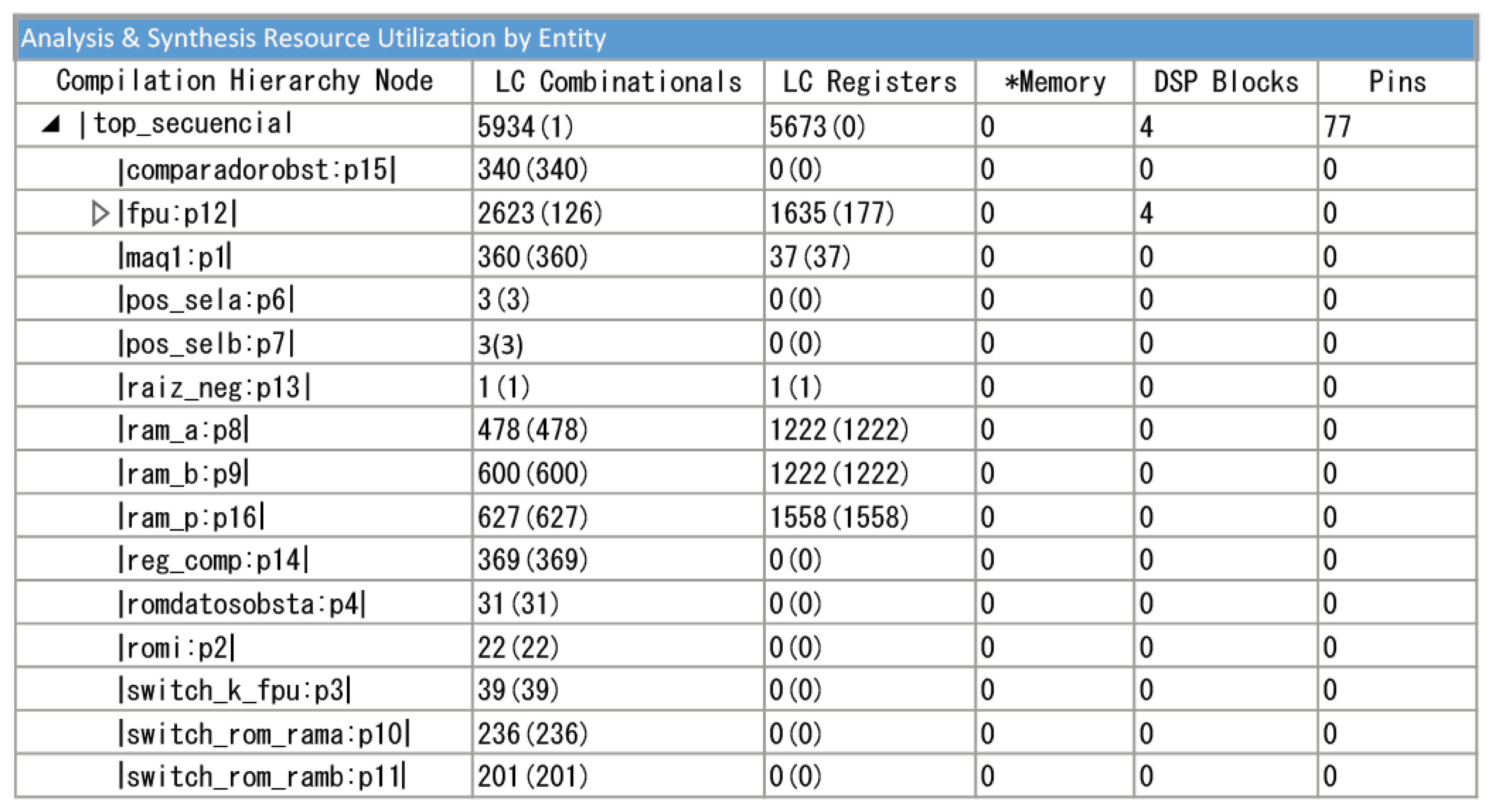
By including the obstacle values present in the environment and executing the algorithms described in Section 4, the FPGA shows a low resource consumption, as can be seen in Figure 15.

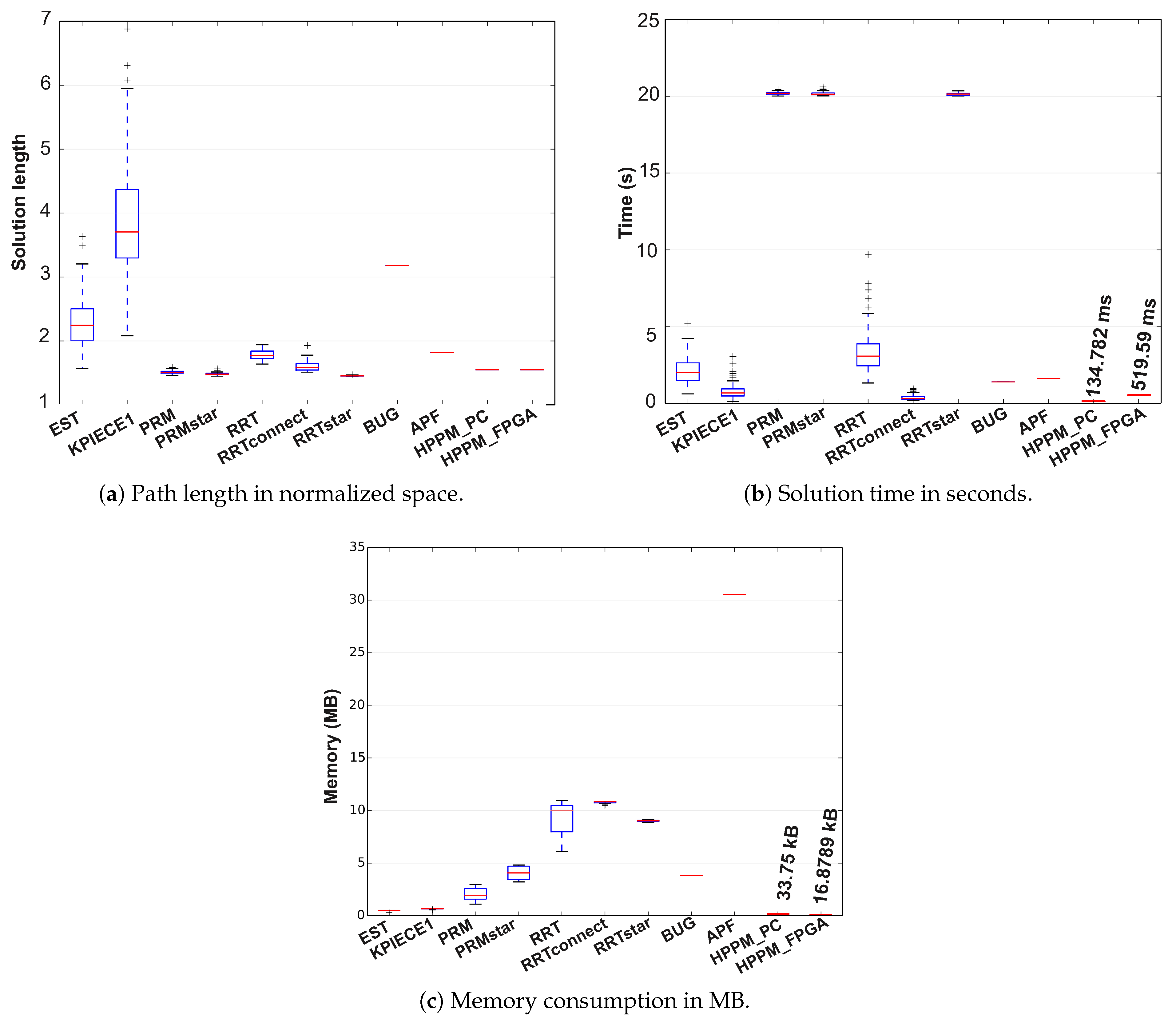
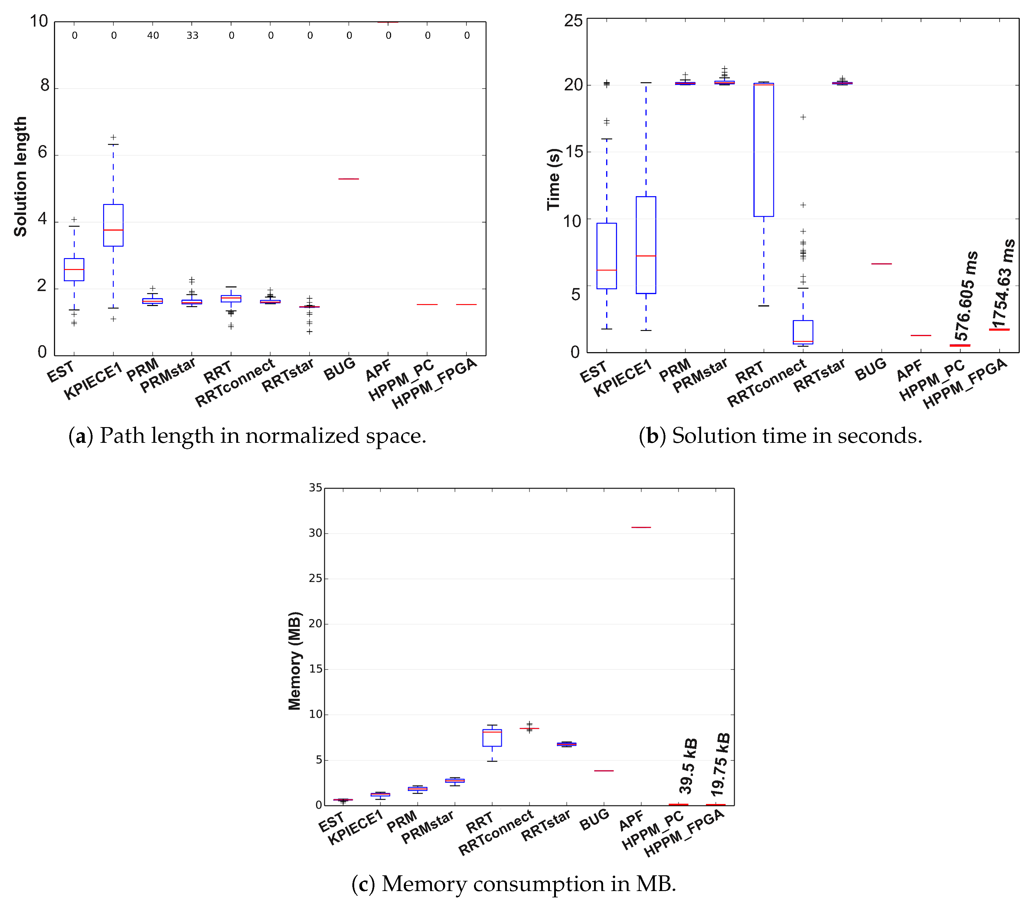
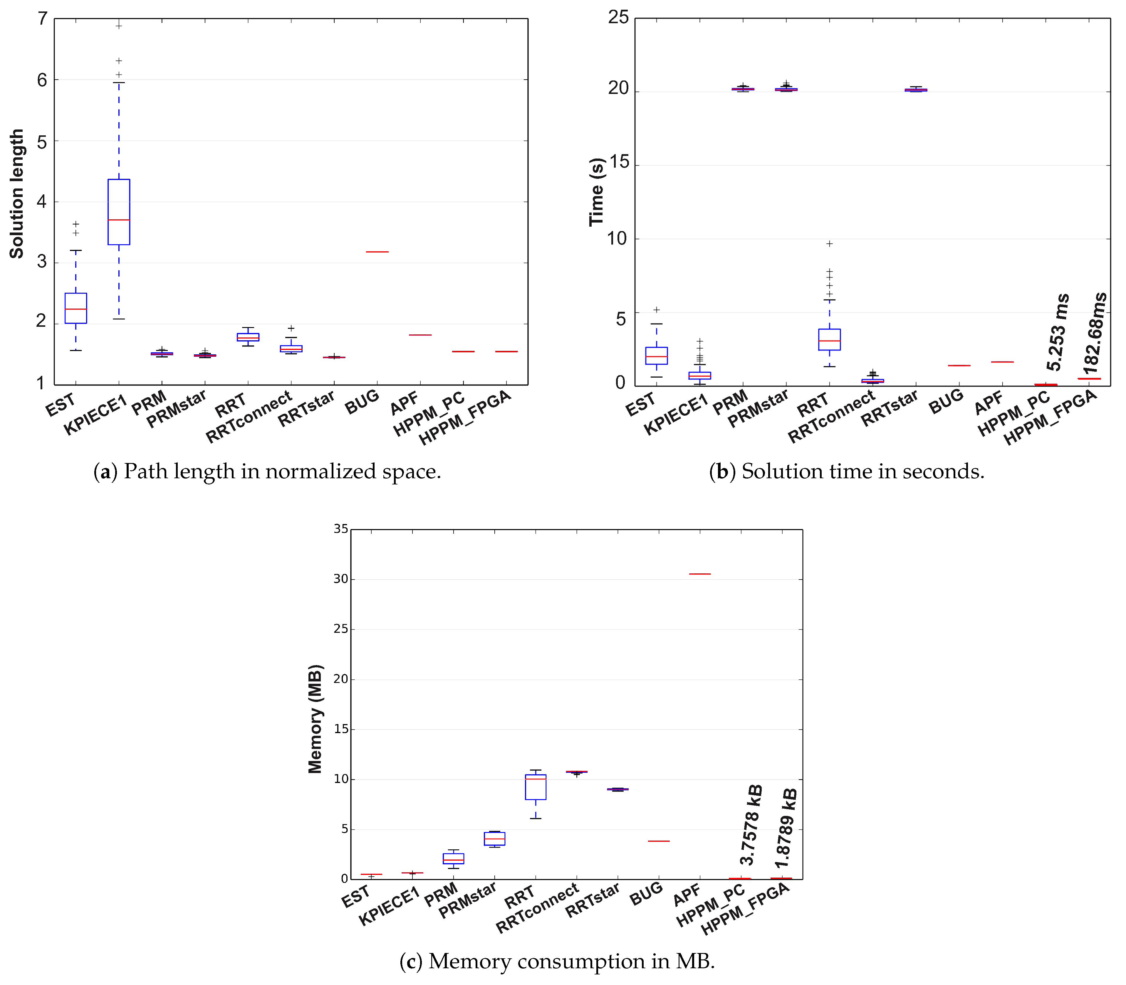
In Figure 16, results of the descriptive statistical analysis for this case are presented using box plots, where the red line represents the median value obtained by executing each sampling-based method 100 times; it can also be noticed that, for some cases, outliers were obtained which are represented by the + signs.

For the case of deterministic methods, only the red line is represented, which is equivalent to the method median and must be compared to other methods’ medians. The proposed implementations in PC and FPGA were compared in terms of path length, simulation time, and memory consumption. Therefore, from Figure 16a, we can conclude that the average distance for compared methods, including the HPPM, is almost similar but EST, KPIECE, and the low DoF Bug algorithm provided longer paths; nevertheless, PRM and RRT_Star methods require, on average, ten times more computation time to solve the same problem (Figure 16b). For this case, the algorithm that provides the best results overall is the HPPM method in both implementations.

As can be seen in Figure 16c, the difference in memory consumption is considerable, whereas the RRT algorithms (including Star and Connect variants) have high memory consumption (close to 10 MB), the HPPM algorithm occupies about 3.7578 kB in PC and just 1.8789 kB in FPGA, turning it into the best option for embedded systems. It is important to notice that APF algorithm needs plenty of memory (close to 30 MB) to get its job done; it requires 8125 times more memory than the implementation in PC and 16,251 times more in FPGA. In addition, 243 times more computation time in PC and 6.67 times in FPGA is needed, which allows us to conclude that HPPM is more robust, efficient, and suitable for low cost embedded systems.

5.2. Case 2

Noticing the advantage in memory usage and reasonable execution time for our implementation in FPGA, an example containing 50 randomly placed obstacles is generated. This time, the configuration scheme that compares the HPPM method to others found in the literature is provided in Figure 17, showing a greater concentration of obstacles and the presence of ellipsoidal obstacles with random rotations, as well as the resulting trajectory of the proposed algorithm.

Again, the comparison of results between the HPPM and other path planning methods is presented. It is worth emphasizing that all the sampling-based algorithms were run 100 times, while the BUG, APF, and HPPM algorithms were run only once; this is because, as already mentioned, they are deterministic methods.

In Figure 18 the results of descriptive statistical analysis of this case are presented using box plots, where the red line represents the median value obtained by executing each sampling-based method 100 times; it can also be observed that, for some cases, outliers were obtained, which are represented by the + signs. For deterministic methods, only the red line is represented, which is equivalent to the method median and must be compared to other methods’ medians.

For this case, EST and KPIECE1 show a good use of resources in terms of memory; nevertheless, they have an inefficient behavior caused by the high variability of the calculated path distance. Furthermore, PRM, PRM Star, and RRT Star algorithms offer optimal distances and reasonable memory usage; the problem is that, to achieve this, they required high runtime, which is not ideal for a real-time execution robot.

Comparing HPPM to the low DoF algorithms, the APF algorithm has acceptable times and path distances but requires too much memory usage to achieve it, while the Bug algorithm maintains a reasonable use of time and memory but obtained paths are not optimal on distance.

In Figure 18c, it can be seen that, despite having reduced memory consumption, the RRT algorithms (original, Star, and Connect versions) are around 10 MB, while PRM algorithms (original and Star) are close to 3 or 4 MB. The results of EST and KPIECE1 methods are close to 1 MB, still superior to the HPPM consumption, which for this case are 33.75 kB in PC and 16.8789 kB in FPGA; therefore, the HPPM algorithm is maintained as the best option for embedded systems.

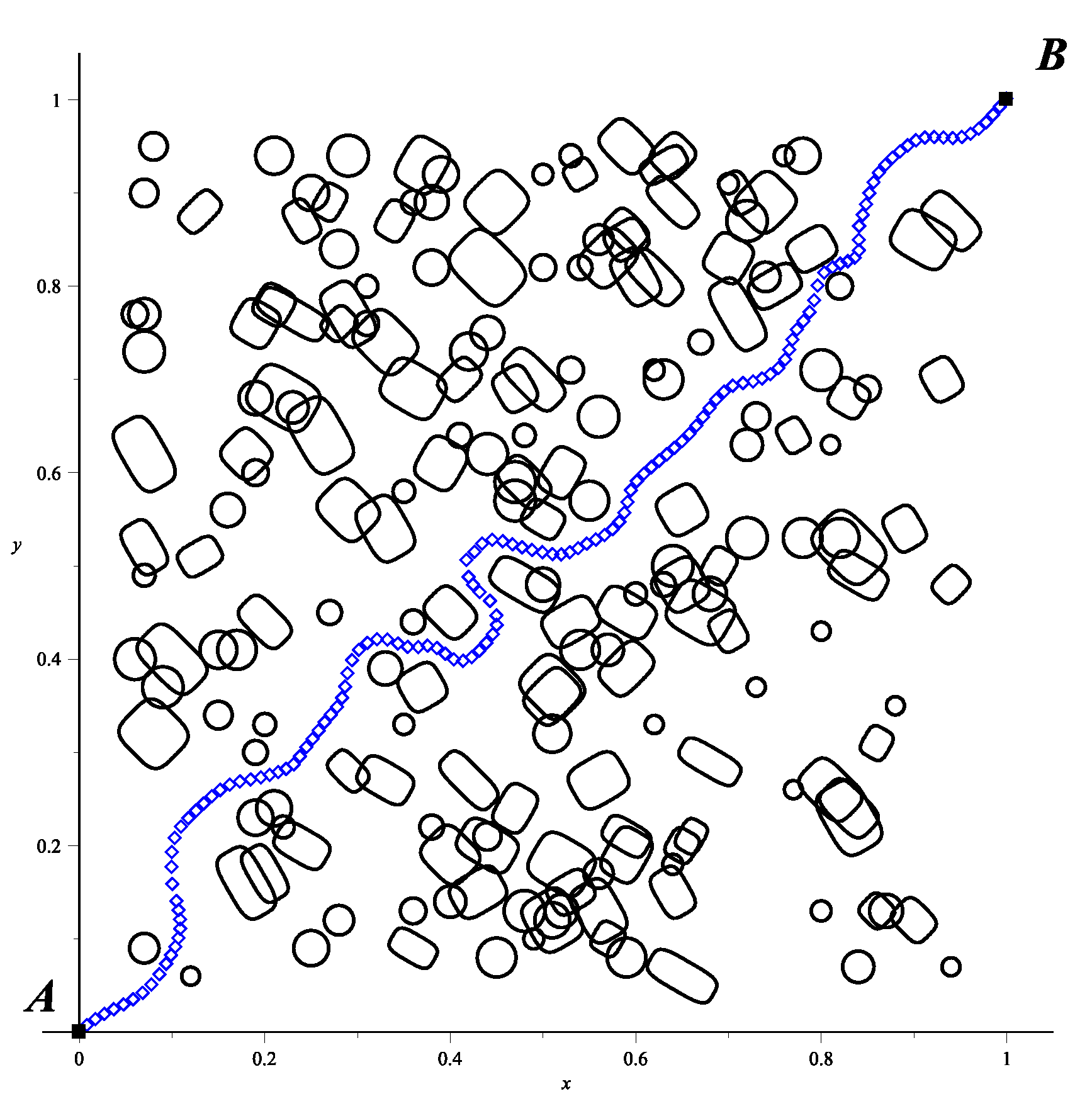
5.3. Case 3

For this case we increase the number of obstacles to 200, aiming to highlight the feasibility of using this methodology in an FPGA given the low memory consumption during the solution process. Obstacles map and the resulting path are depicted in Figure 19.

For this particular example, all the sampling-based algorithms were run 200 times, because some of the methods could not converge to a solution. It is remarked that the BUG, APF, and HPPM algorithms were executed only once, knowing that their deterministic condition forces them to obtain the same result regardless of the number of times they are executed.

Finally, in Figure 20 results of the descriptive statistical analysis of this last case are presented using box plots, where the red line represents the median value obtained by executing each sampling-based method 200 times; it can also be observed that, for some cases, outliers were obtained, which are represented by the + signs. For deterministic methods, only the red line is represented, since it is equivalent to the method median and must be compared to other methods’ medians.

As the number of obstacles increase, low DoF algorithms tend to find solutions with paths that are too long (Figure 20a). Otherwise, the EST and KPIECE1 algorithms practically double the path size with respect to the other algorithms.

Taking into account execution time, most methods need a large amount of time to ensure an adequate response, as can be seen in Figure 20b; methods with the shortest execution times were the RRT Connect, the APF method, and the HPPM where it can be highlighted that the HPPM algorithm uses less than a second in PC.

Regarding the use of memory, the APF method needed a large amount of memory for its execution, about 30.685 MB (Figure 20c), the RRT algorithms exceed 5 MB, and the rest required, at least, 1 MB. Therefore, HPPM implementation (PC and FPGA) remains as the best option for embedded systems using 71.6 kB and 408 kB, respectively.

6. Discussion

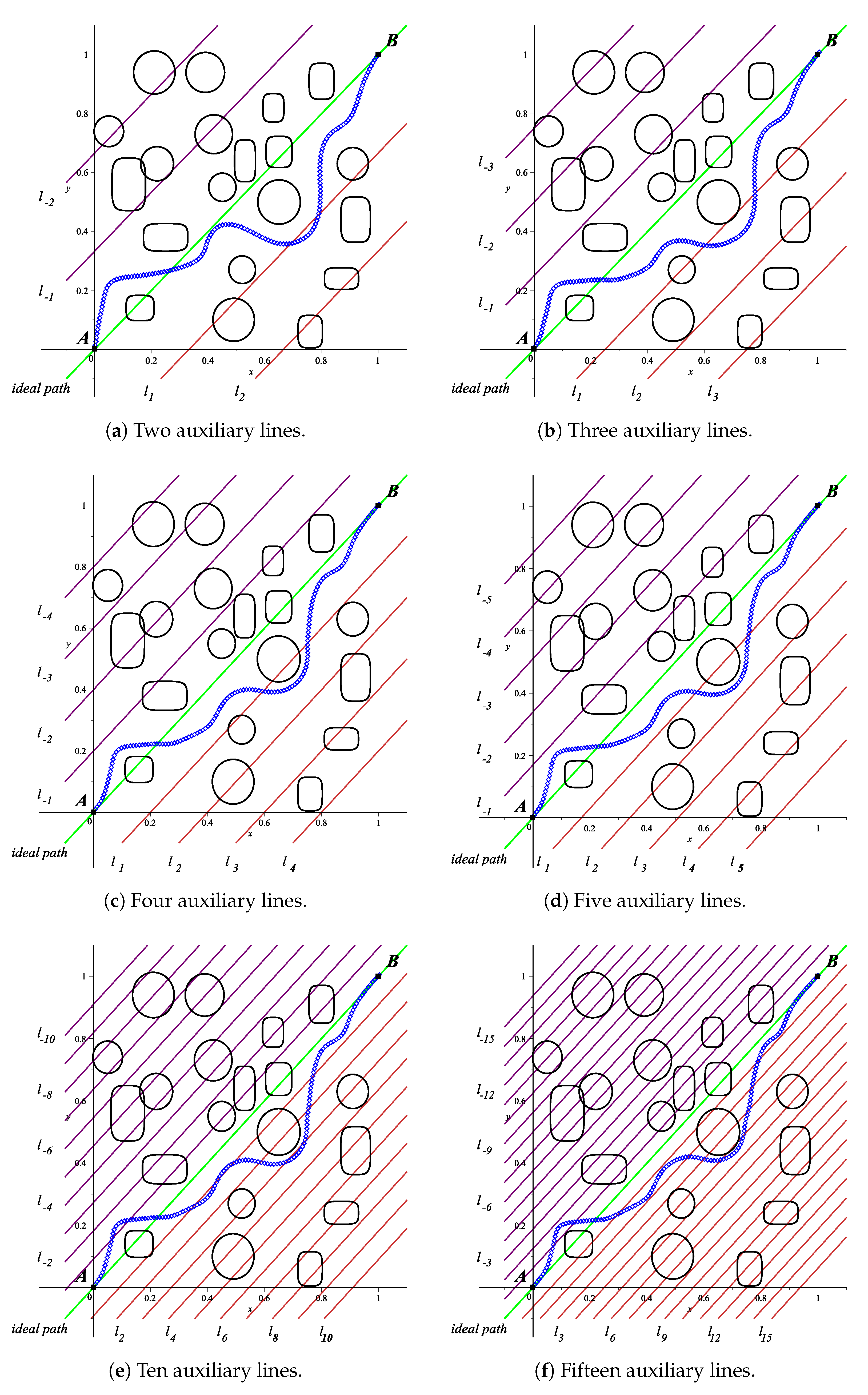
From literature [31], we know that users should have deep knowledge for the repulsion parameter assignment process. Nevertheless, our proposal aims to circumvent such a cumbersome manual process. What is more, during the repulsion parameter assignment process, there exists a relationship between the number of auxiliary lines and execution time that depends on the available hardware. In fact, we found in Section 3.1 that four auxiliary lines per side of the ideal path are enough to provide an optimized collision-free path. We found that more than four auxiliary lines increases the computation time and the memory requirements without noticeably improving the collision-free path. Results from the methods described above are summarized in

Table 4. Comparative median results of Execution Time (ET), Normalized Path Length (NPD), and Median Memory Consumption (MMC).

	20 Obstacles				50 Obstacles				200 Obstacles
Method	ET (s)	NPD	MMC (MB)		ET (s)	NPD	MMC (MB)		ET (s)	NPD	MMC (MB)
EST	0.519	2.863	0.332		3.214	2.210	0.404		4.388	2.533	0.498
KPIECE	0.331	3.634	0.710		0.368	3.360	0.597		5.199	3.727	0.597
PRM	10.132	1.607	2.837		20.114	1.494	2.031		20.226	1.554	1.775
PRM_Star	10.117	1.586	5.695		20.130	1.480	4.017		20.125	1.598	2.646
RRT	1.211	1.936	7.443		2.858	1.702	8.289		13.399	1.727	6.560
RRT_Connect	1.286	1.898	8.074		0.402	1.584	10.654		4.499	1.669	8.355
RRT_Star	10.157	1.584	9.062		20.133	1.452	8.996		20.167	1.236	6.753
BUG	1.468	6.955	3.861		1.4	3.179	3.837		6.64	5.294	3.849
APF	1.215	1.505	30.535		1.642	1.819	30.541		1.273	9.992	30.685
HPPM_PC	0.005	1.428	0.003		0.134	1.548	0.032		0.576	1.530	0.038
HPPM_FPGA	0.182	1.430	0.002		0.519	1.549	0.016		1.754	1.530	0.019

.

As can be observed, FPGA implementation of HPPM remains as the best option for a path planning method in terms of memory consumption, while keeping itself as a competitive method in terms of distance and solution time. In general terms, the methods that obtain slightly smaller distances than HPPM face the problem of requiring noticeable higher execution times and memory consumption. Therefore, HPPM is an ideal algorithm for embedded systems.

Low DoF algorithms tend to use simple criteria to achieve their goal, which makes them efficient when the number of obstacles is minimal or there is a wide free space. Nevertheless, if numerous obstacles are found within the environment, having different dimensions, map resolution tends to be increased generating large consumption of memory and time to find the solution. In addition, since they do not have an optimization adjustment, they may find solutions that are too long or complex. In general, APF method requires high memory consumption for its execution and the Bug algorithm maintains a stable consumption, although higher than HPPM.

For some methods, like EST and KPIECE, despite having consumed relatively low memory, they tend to produce longer trajectories. On the other hand, RRT method and its variants provide acceptable trajectories but memory consumption tends to be high during its execution. In contrast, HPPM (which executes only once) generates acceptable trajectories with reasonably low memory consumption. Besides, since the probabilistic methods produce a great variation in the results every time they are executed, it was necessary to run 200 simulations to obtain the median values, thus eliminating the influence generated by atypical values of low performance or failed simulations.

In fact, when free space is limited, a certain percentage of these simulations find no solution; therefore, the use of such algorithms is impractical in embedded systems where low computing resources do not allow their real-time execution, or simply cannot be implemented. Proof of this is the case of 200 obstacles, where PRM methods (original and Star) fail to find the solution at 30% because they run out of time, while RRT methods (original and Star) find an approximate solution 10% of the time, instead of the exact solution.

According to the HPPM algorithm itself, in PC and FPGA, the generated trajectory is almost identical. There is a slight difference in PC because its processor architecture works using 64 bits, while FPGA architecture is 32 bits. Architecture difference is reflected in memory consumption since the PC consumes 3.76 kB for 20 obstacles, 33.75 kB for 50 obstacles, and 39.5 kB for 200 obstacles, while the FPGA consumes 1.88 kB, 16.88 kB, and 19.75 kB, respectively. In addition, while working in PC, calculations can be obtained with higher precision; this means that the number of iterations achieved by the calculations of predictive and corrective values during path generation are greater than the amount reached in calculations with 32 bits.

Another relevant aspect is the execution time; the HPPM developed in the PC shows greater advantage over the other methods. Even more, applying this methodology in an embedded system (FPGA), the execution time of the HPPM is only comparable to KPIECE method in PC; nevertheless, KPIECE obtains, as a recurring result, a longer path.

Although the FPGA computation time in the implementation for 20 obstacles is similar to the different methods, it is important to emphasize that for 50 and 200 obstacles computation times are surprisingly competitive compared to the random tree techniques simulations; besides, it must be considered that the FPGA power consumption is considerably lower (below 50% with respect to the use of PCs, see Table 1). The importance of this research lies in the fact that other techniques reported in the literature, to the author’s best knowledge, do not have the implementation of these conditions using an FPGA, probably because of the notable high power demand, execution time, and memory consumption required by these methods.

An advantage lies in the fact that obstacle representation in HPPM influences a single equation within the system. If obstacle number increases, the number of equations to be solved remains the same; only one of the terms for this system of equations becomes extensive (with a linear relationship to the number of obstacles). In addition, the equation does not present alterations due to the obstacle size, a circumstance that affects the low DoF algorithms. When small obstacles increase, these algorithms are forced to reduce the cell size, increasing the resolution of the map to be solved.

Another advantage is the fact that it is a deterministic method, reducing the number of calculations because it focuses on a single solution in terms of trajectory, which is contrary to what happens with the sampling-based algorithms. All expansion trees depend on the calculation of a set of possible expansion points, combined with an optimization criterion in the selection of the next trajectory step.

Random tree methods increase their memory and computation time exponentially due to two fundamental aspects: each random point during the process must be stored to be employed later on the path generation phase which implies a notable memory consumption and the collision checking process that consumes most of the CPU time.

On the other hand, memory and computation time of the homotopy continuation methods increase linearly with respect to the number of obstacles as depicted in [31]. In fact, homotopy continuation method is deterministic, providing a single collision-free path using a numerical continuation process. What is more, the proposed scheme based on homotopy does not require any collision checking stage because it ensures zero-collision probability due to its mathematical formulation.

7. Concluding Remarks and Future Work

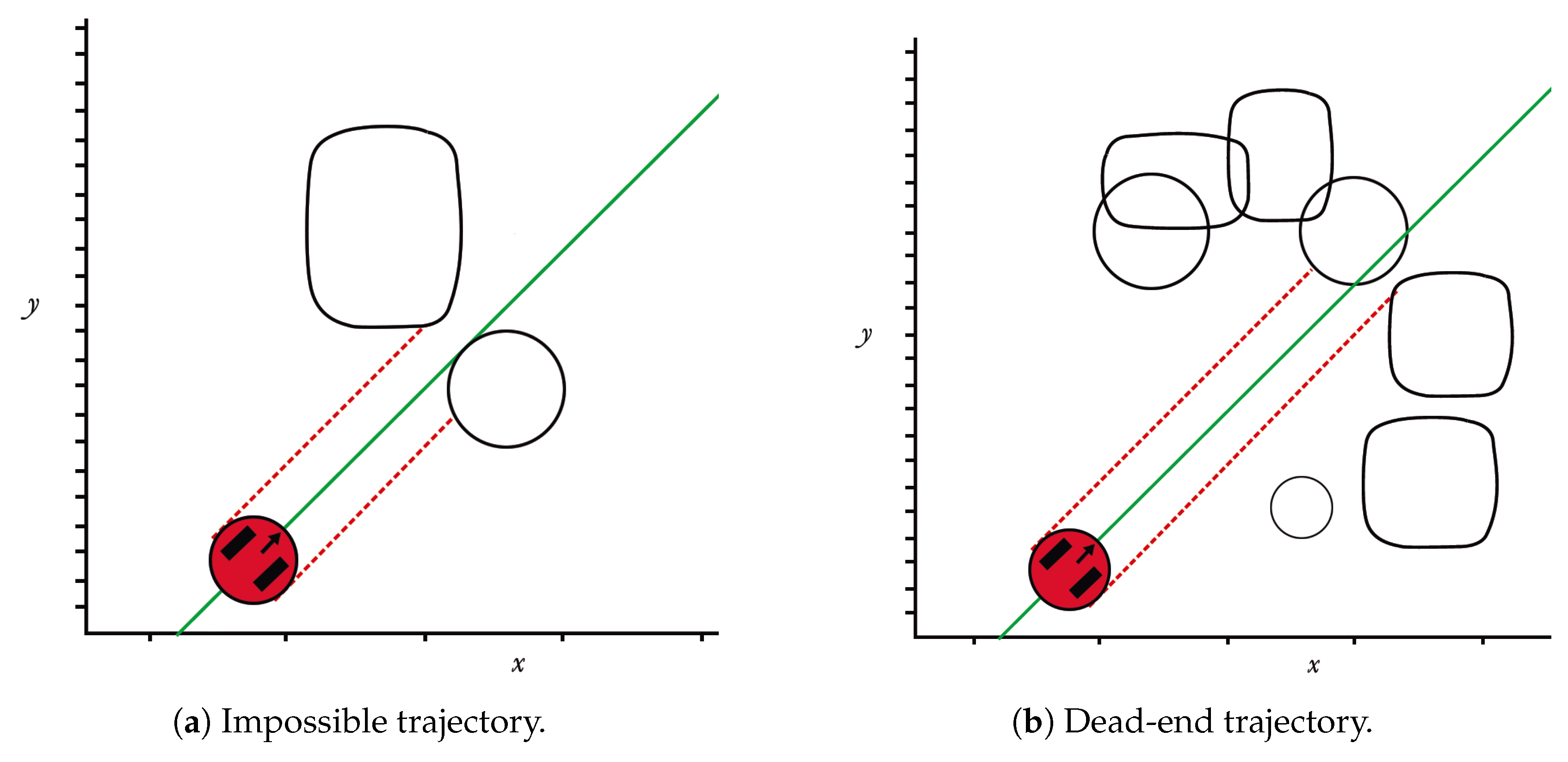
An improvement to the standard HPPM methodology was presented, which consists of a new method for calculating the repulsion parameter, aiming to achieve the shortest distance path. In addition, an analysis of neighbourhoods was included, which ensures that the trajectory moves around spaces that may compromise its continuity, avoiding any dead-end issue.

The implementation was tested in a very low resource FPGA, which demonstrated competitive computing times in relation to implementations of PC sampling techniques, allowing one to conclude that the proposed methodology is viable to solve practical cases in real time on embedded systems, therefore offering the possibility of generating implementations at a very low cost.

Moreover, it will be worthwhile to apply this methodology in closed environments and under the existence of narrow corridors since they are usually the most complicated environments for the methods based on random sampling techniques. In addition, this opens the possibility to perform experimental tests with differential type robots, not holonomic or omnidirectional and with multiple degrees of freedom.

In this investigation, all the calculations were carried out sequentially; nevertheless, we believe that, as future work, we can take advantage of parallel implementation of homotopy methods as those reported in [46,47] to reduce computation time. In addition, we can evaluate in parallel the symbolic expressions found during application of the Newton-Raphson algorithm (corrective step) of the numerical continuation.

As future work, the algorithm will be tested in real-time situations with dynamic obstacles. In addition, this methodology will be applied in multiagent schemes, allowing collaborative work without risks of mutual collision. Furthermore, algorithm implementation in applications to real-life problems is desired, like car automatic driving control system. Finally, future work will aim to implement and compare this methodology in three-dimensional environments, as presented in [6,19].