Electrical Damping Assessment and Stability Considerations for a Highly Electrified Liquefied Natural Gas Plant


Abstract
:1. Introduction
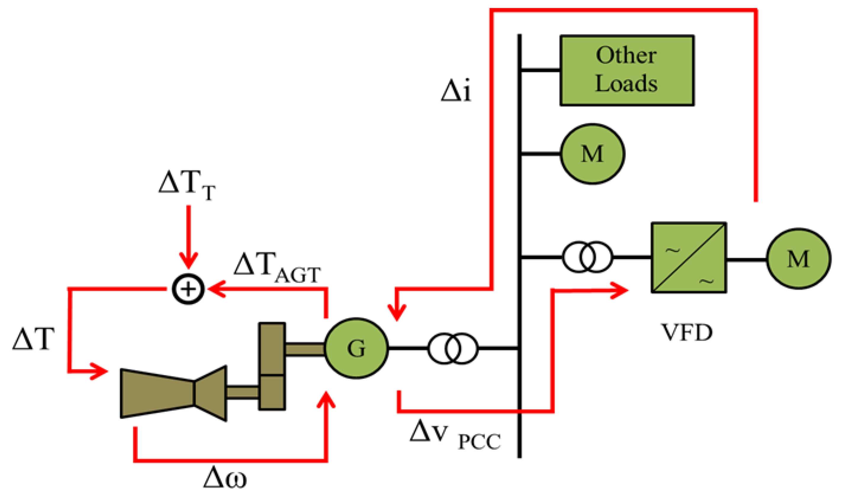
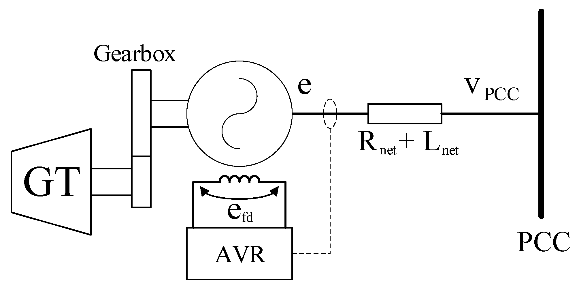
2. Case Study
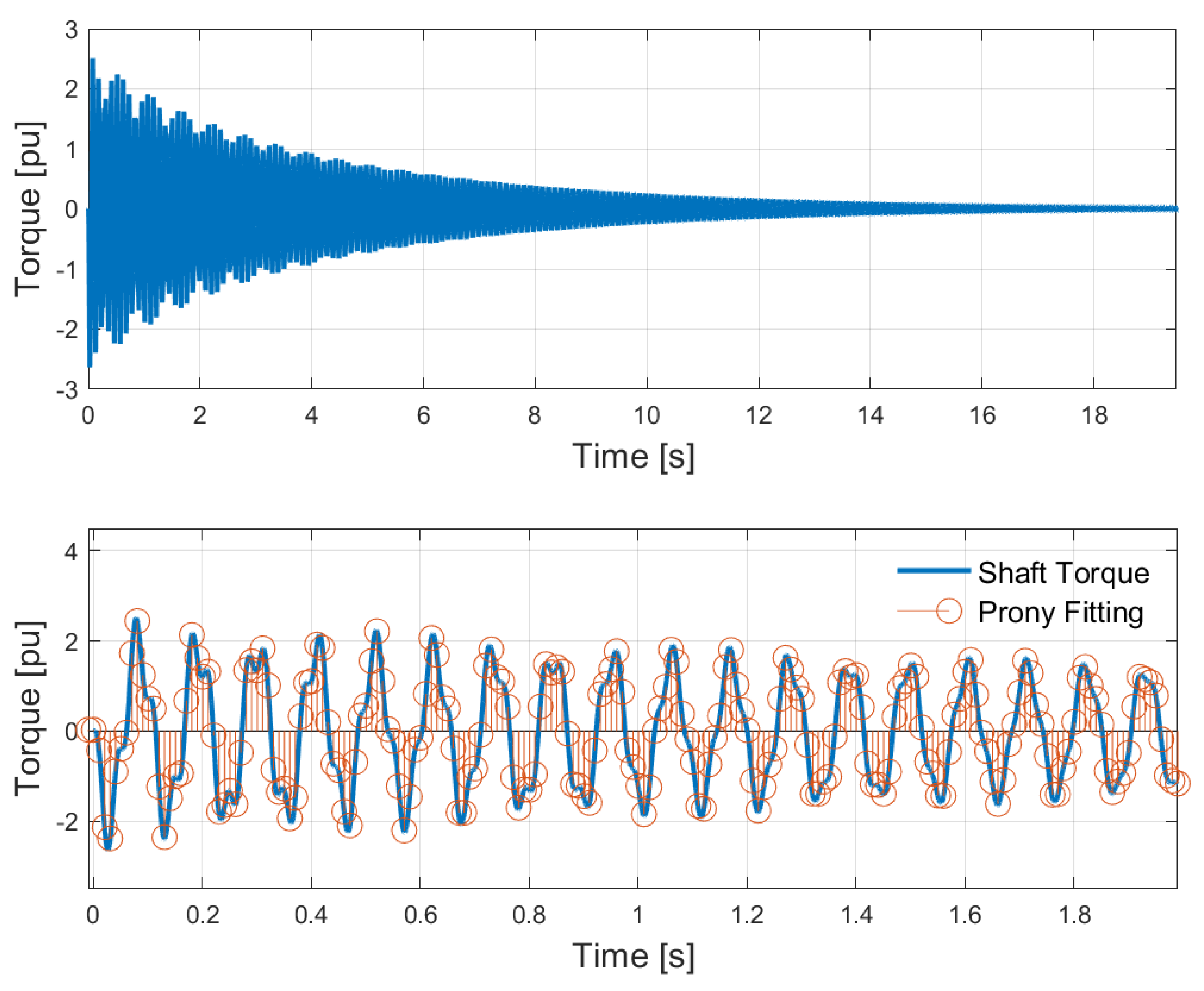
3. Sub-Synchronous Torsional Interaction Phenomena
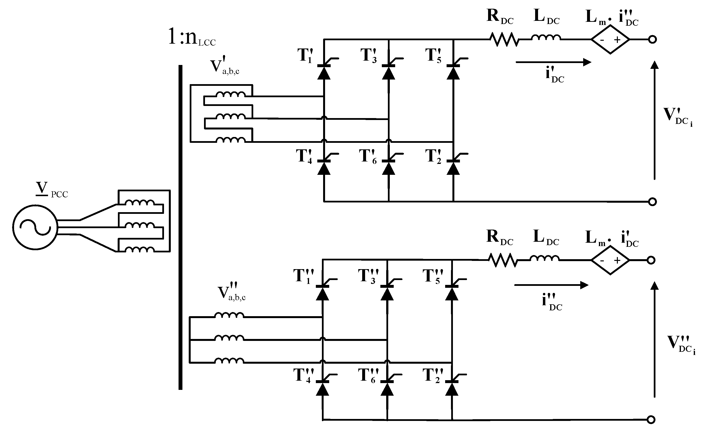
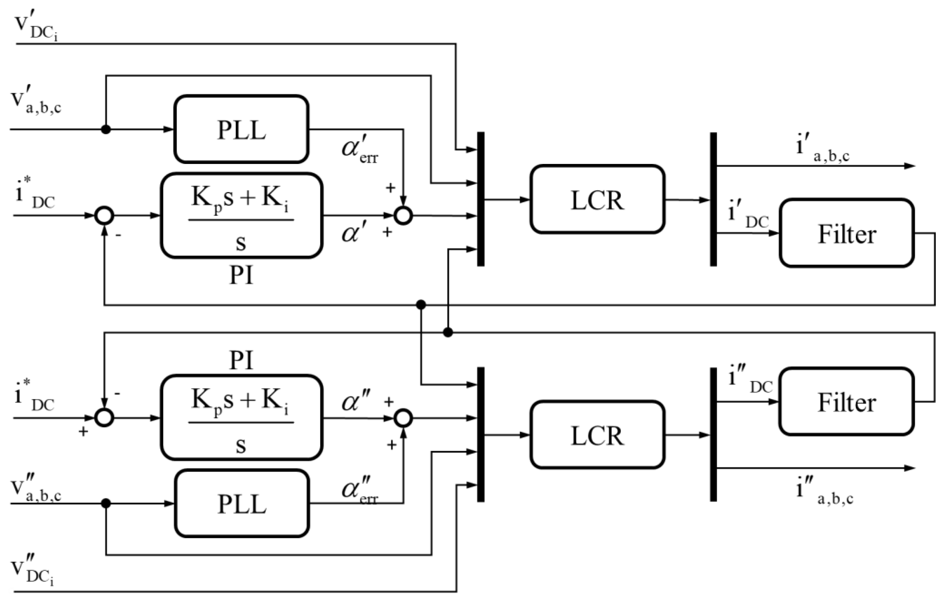
4. Model and Control of the Thyristor Variable Frequency Drive
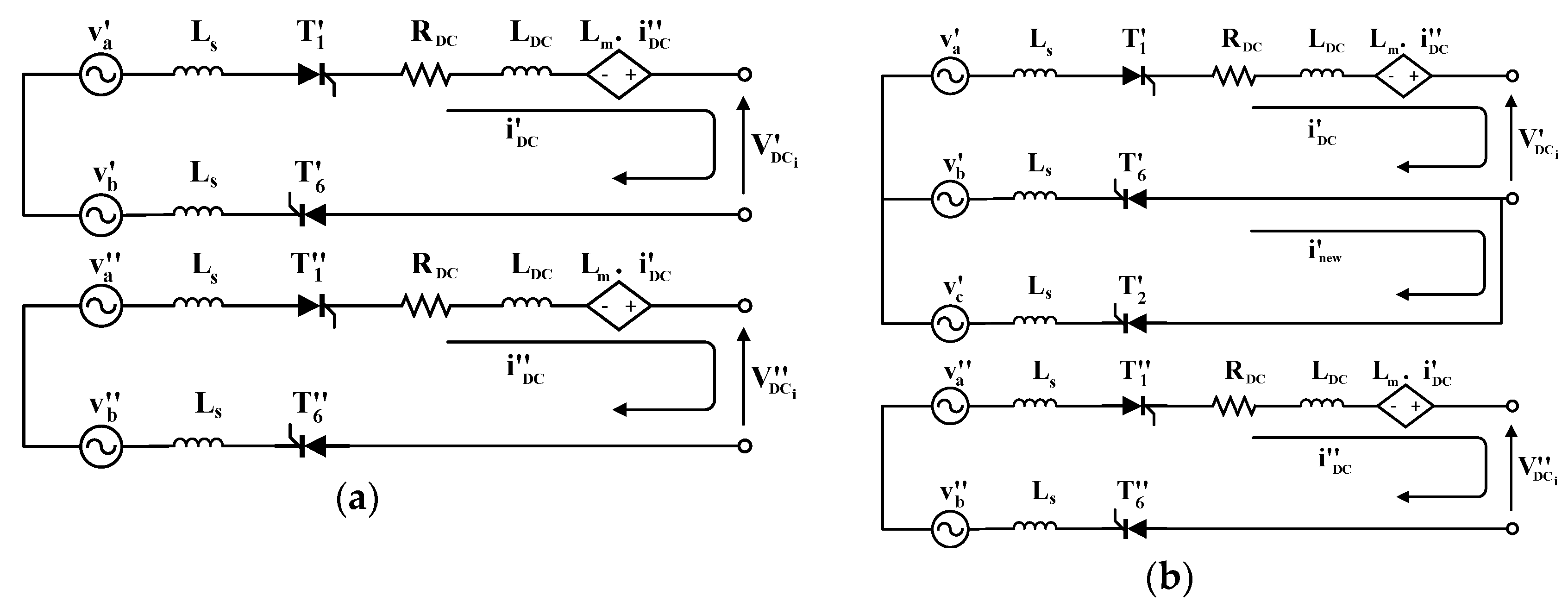
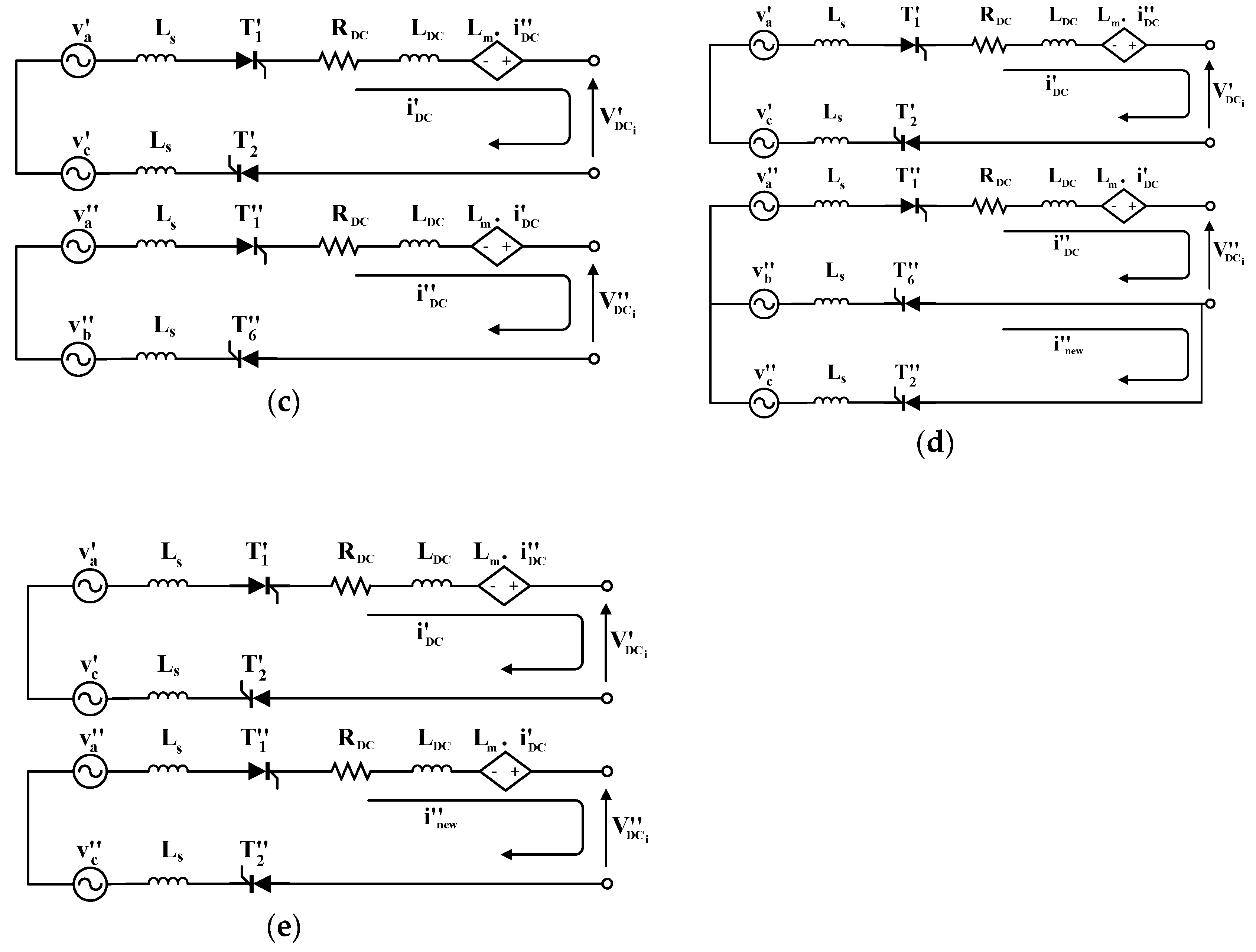
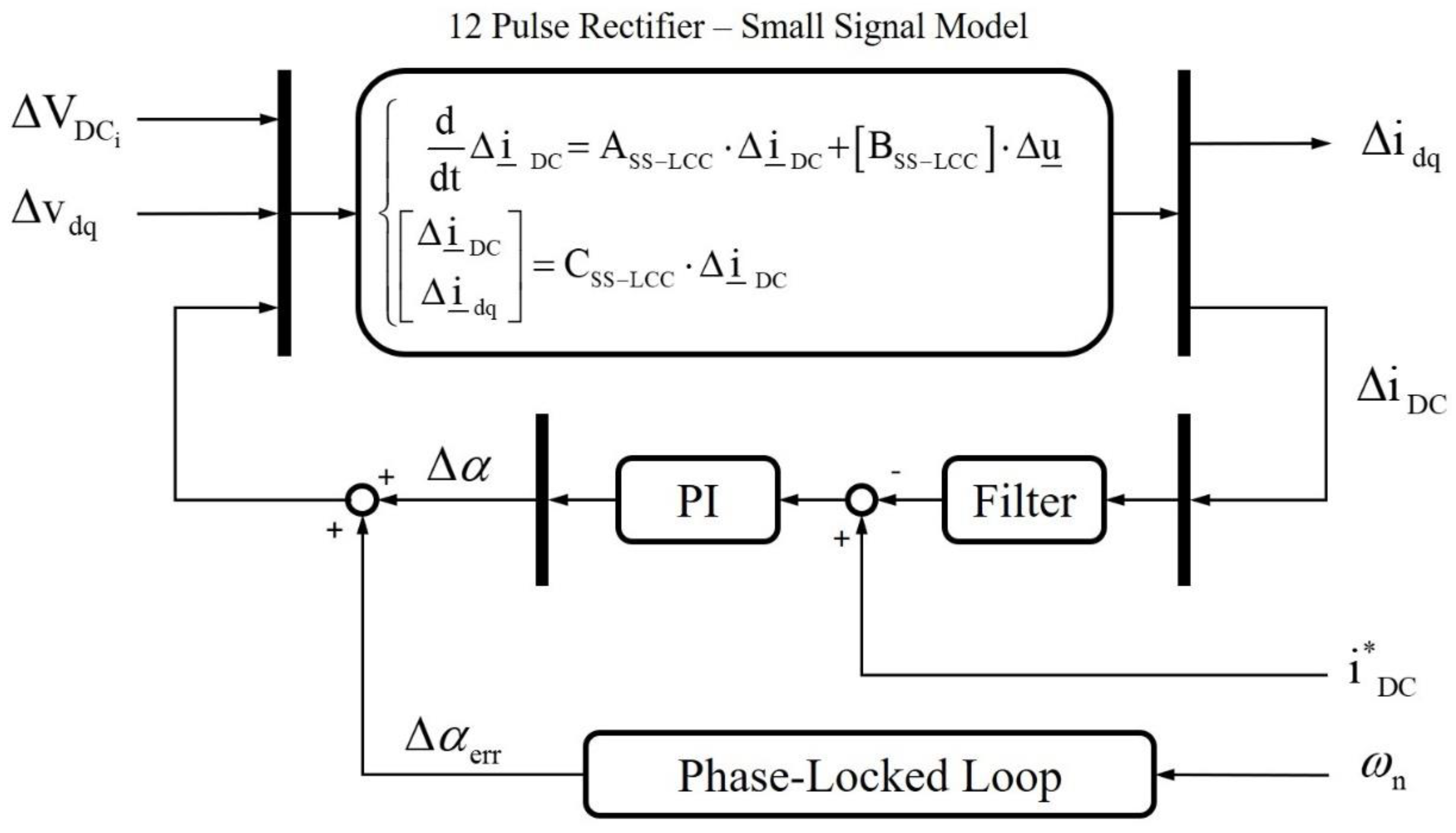
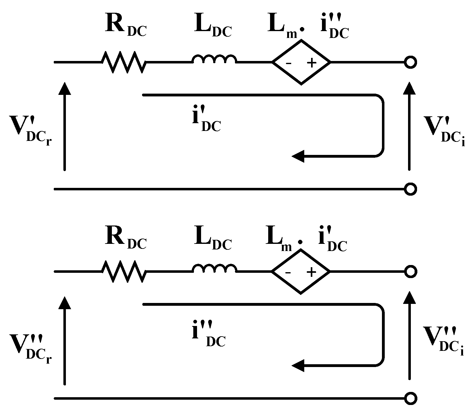
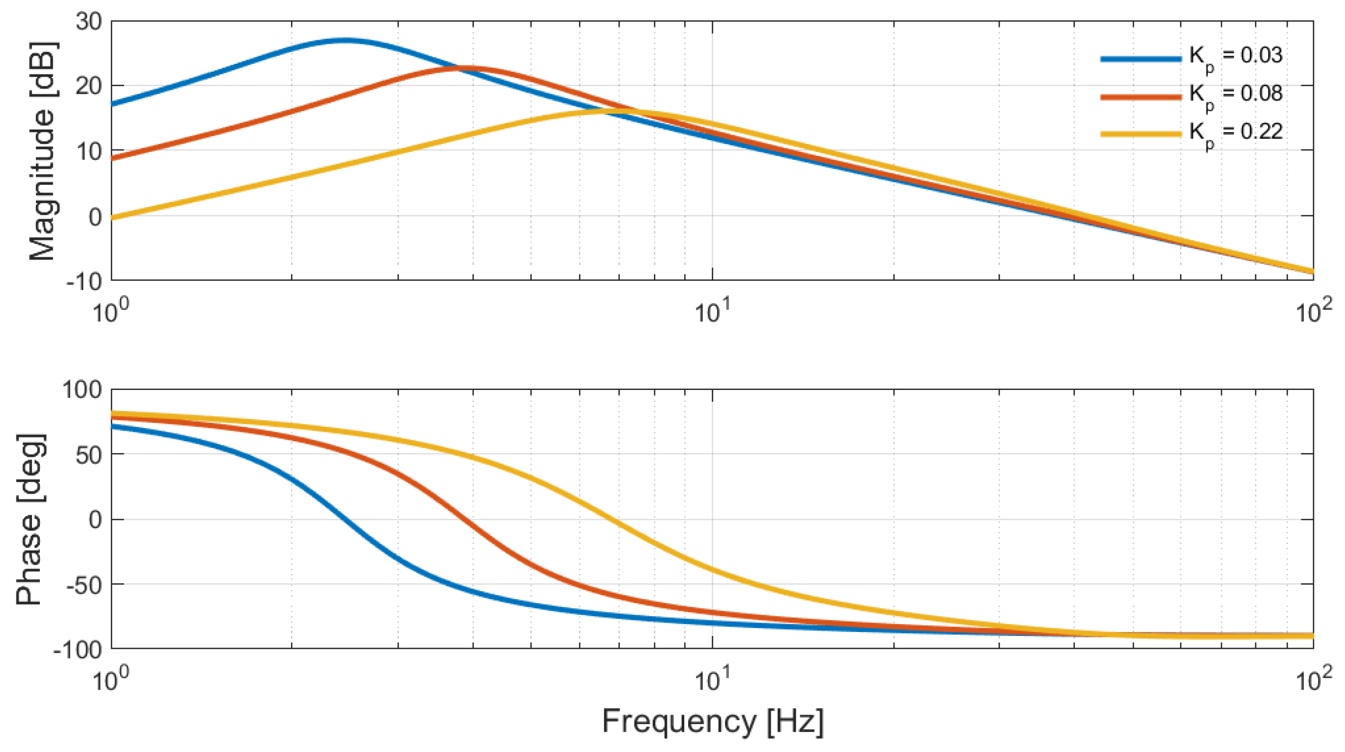
4.1. Small-Signal Model of the AC/DC Power Conversion Stage
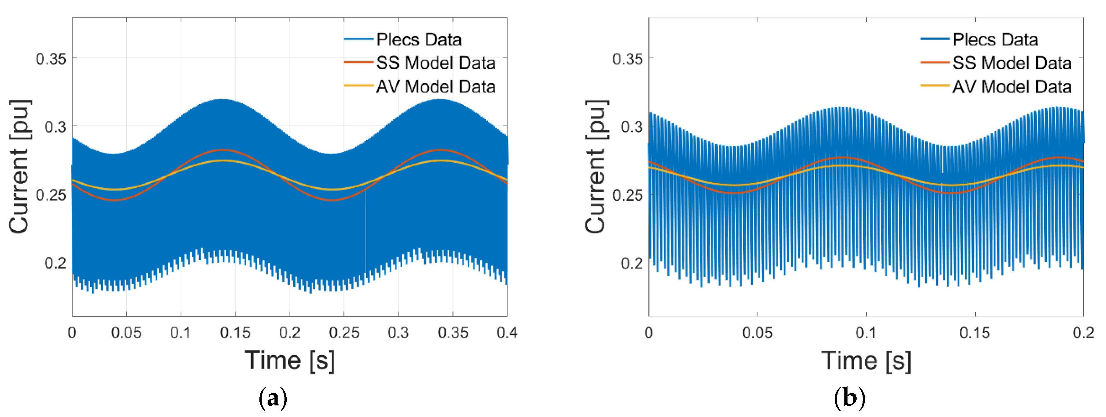
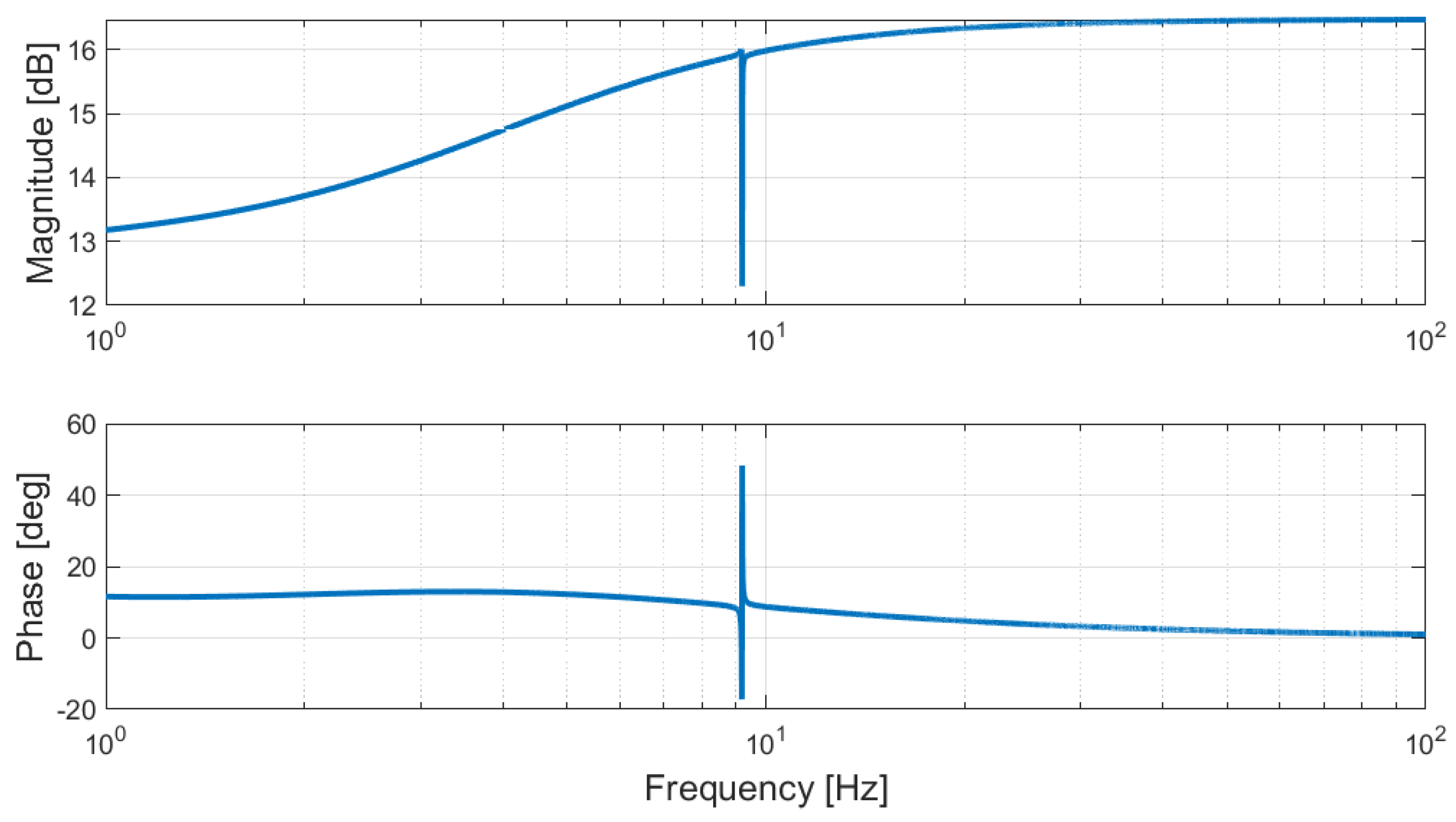
4.2. Model Validation of the AC/DC Power Conversion Stage
5. Model and Control of the Turbine-Generator Unit
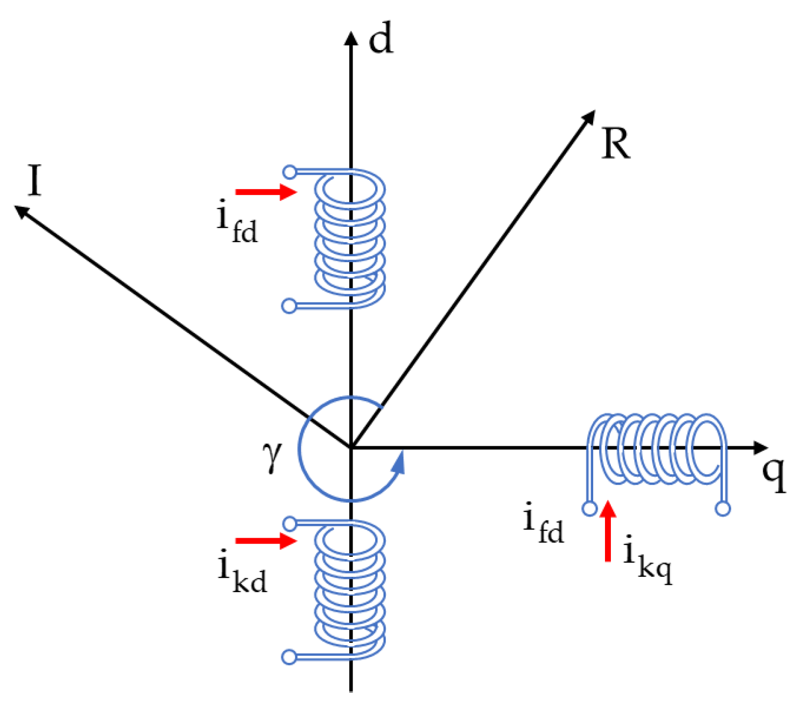
5.1. Small-Signal Model of the Synchronous Generator
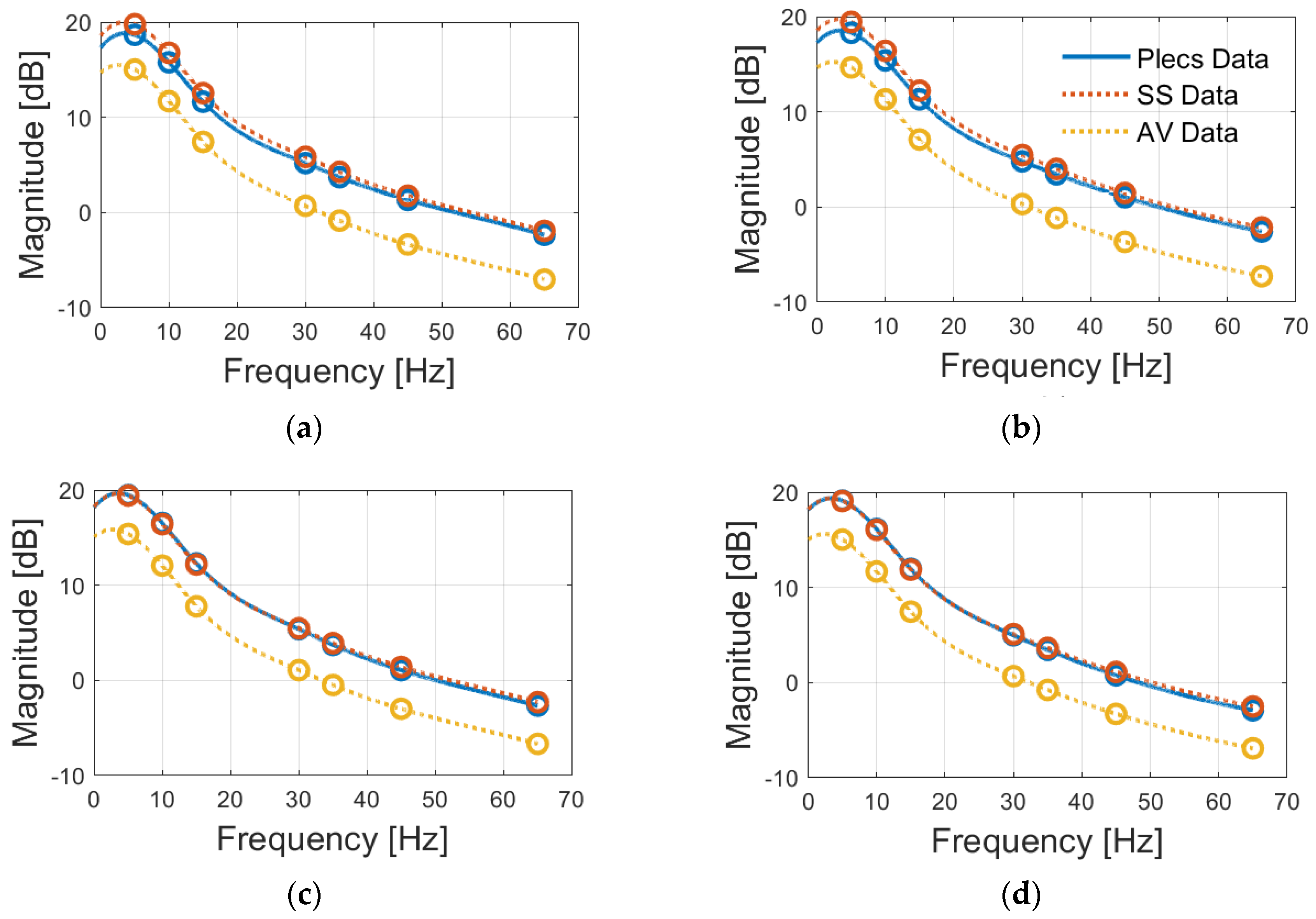
5.2. Model Validation of the Synchronous Generator
6. Damping Assessment and Stability Considerations
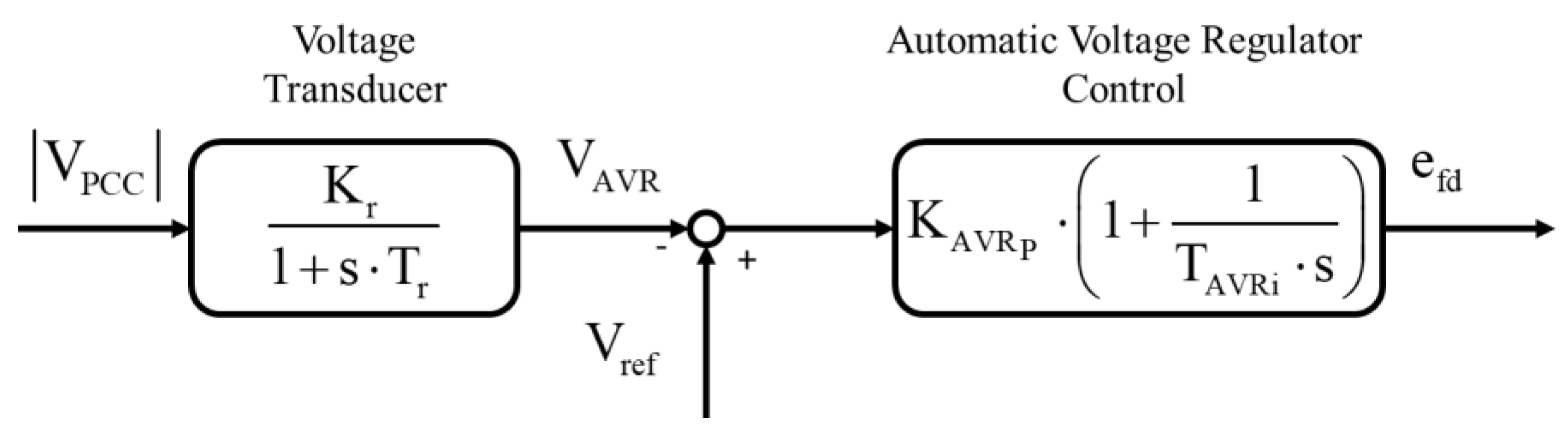
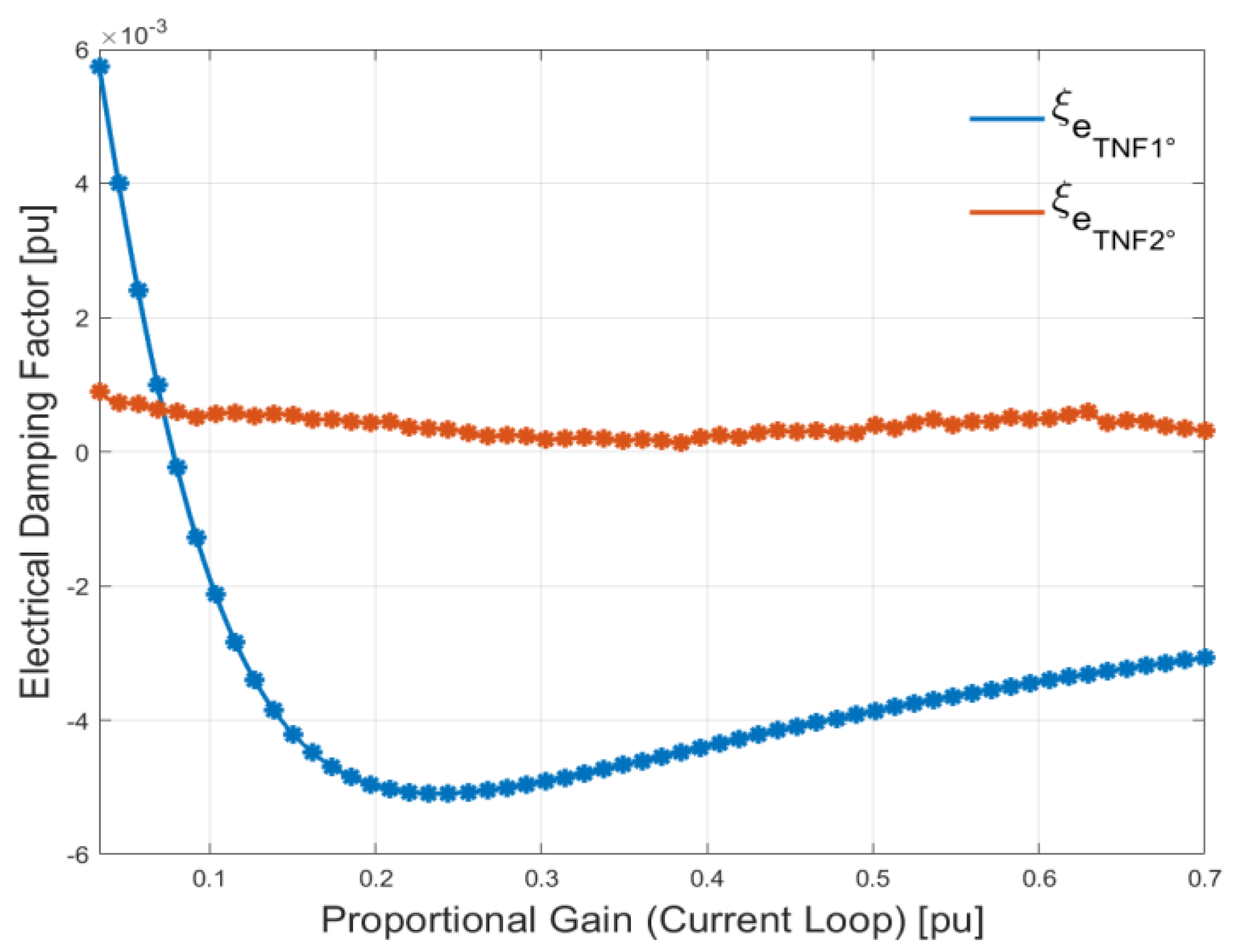
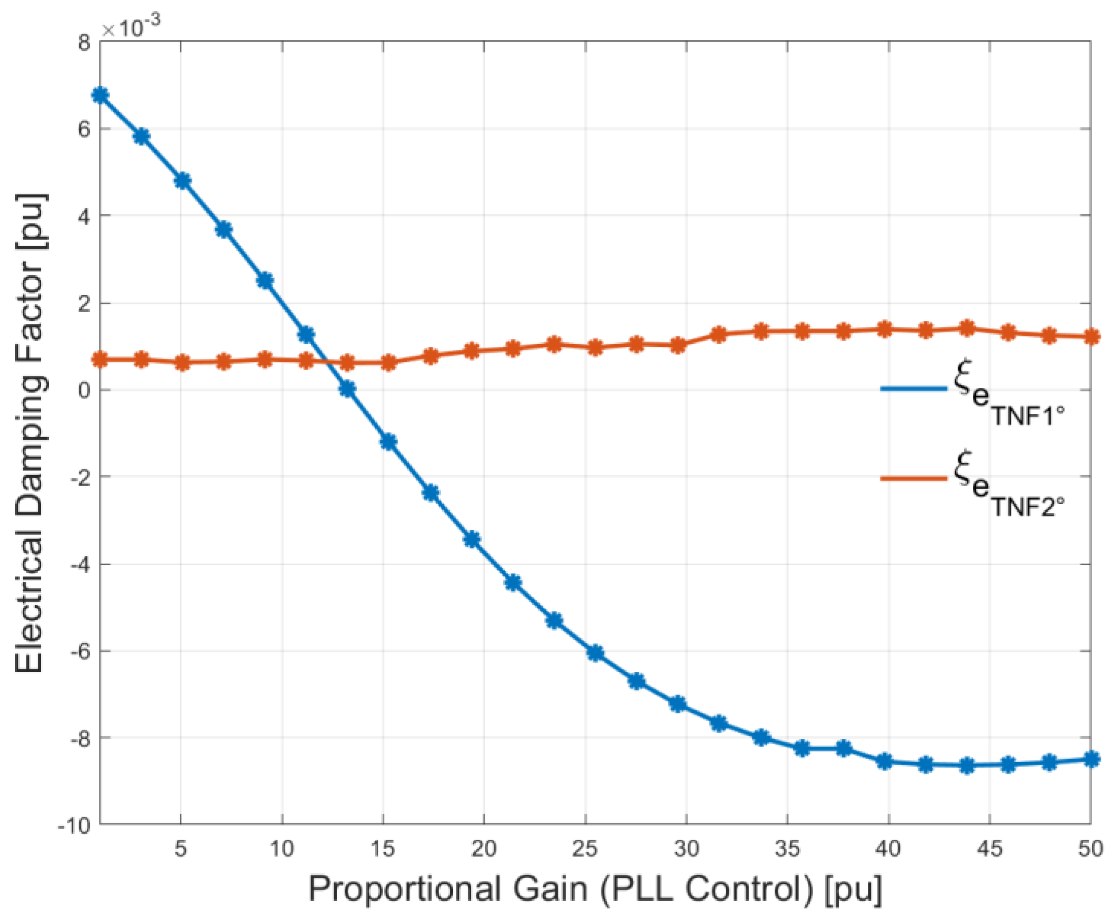
6.1. Electrical Damping Assessment
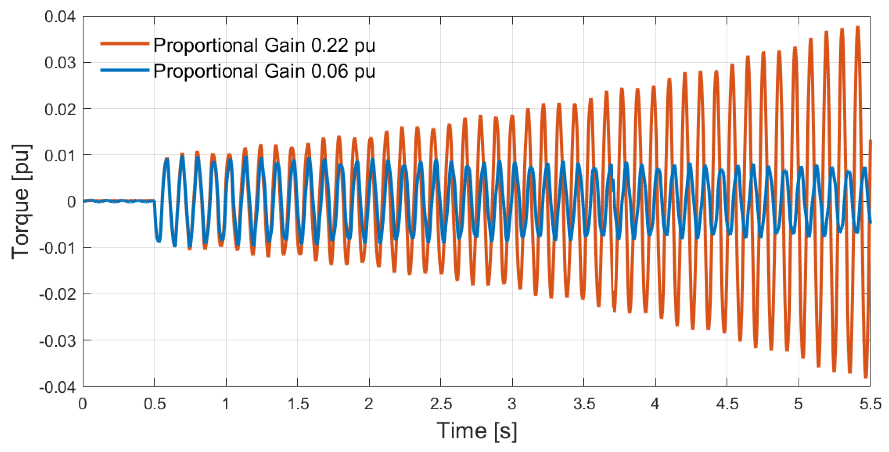
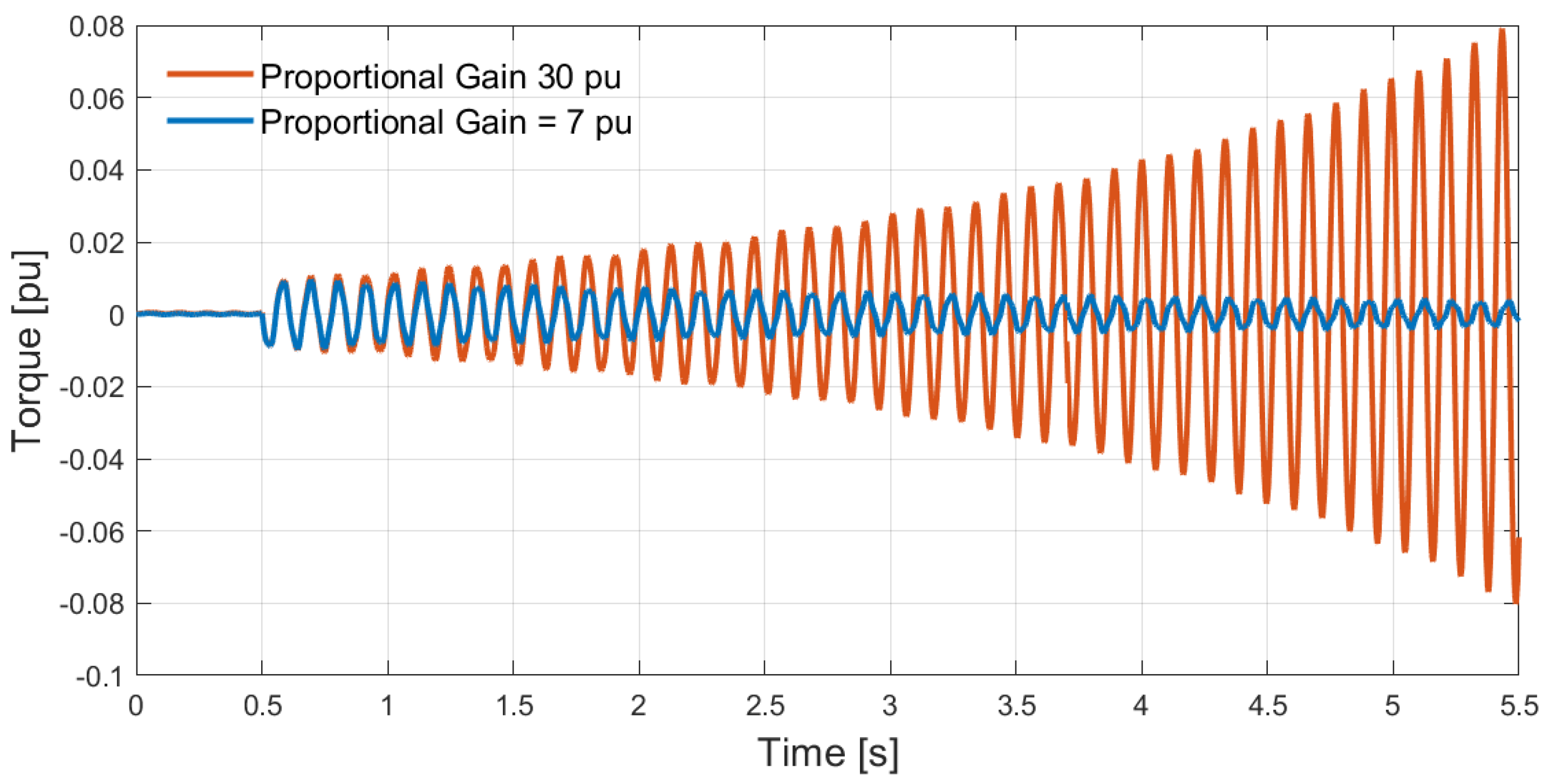
6.2. Stability Evaluation
7. Conclusions
Author Contributions
Funding
Acknowledgments
Conflicts of Interest
Appendix A
References
- Bongini, L.; Mastromauro, R.A. Sub-synchronous torsional interactions and start-up issues in Oil&Gas Plants: A real case study. In Proceedings of the 2019 AEIT International Annual Conference (AEIT), Florence, Italy, 18–20 September 2019; pp. 1–6. [Google Scholar] [CrossRef]
- Svetti, F.; Rotondo, P.; Sgrò, D.; Meucci, F. Practical guideline for Oil&Gas design against sub-synchronous torsional interaction phenomena. In Proceedings of the Turbomachinery and Pump Symposia, Houston, TX, USA, 14–17 September 2015; pp. 1–13. [Google Scholar]
- Harnefors, L. Analysis of subsynchronous torsional interaction with power electronic converter. IEEE Trans. Power Syst. 2007, 22, 305–313. [Google Scholar] [CrossRef]
- Schramm, S.; Sihler, C.; Song-Manguelle, J.; Rotondo, P. Damping torsional interharmonic effects of large drives. In Proceedings of the 2009 IEEE 6th International Power Electronics and Motion Control Conference, Wuhan, China, 17–20 May 2009; pp. 484–490. [Google Scholar] [CrossRef]
- Sihler, C. Suppression of torsional vibrations in rotor shaft systems by a thyristor controlled device. In Proceedings of the 2004 IEEE 35th Annual Power Electronics Specialists Conference, Aachen, Germany, 20–25 June 2004; pp. 1424–1430. [Google Scholar] [CrossRef]
- Sihler, C.; Schramm, S.; Song-Manguelle, J.; Rotondo, P.; del Puglia, P.S.; Larsen, E. Torsional mode damping for electrically driven gas compression trains in extended variable speed operation. In Proceedings of the 38th Turbomachinery Symposium, Houston, TX, USA, 14–17 September 2009; pp. 81–92. [Google Scholar]
- Sannino, A.; Liljestrand, L.; Rothman, B.; Nestli, T.; Kjall-Ohlsson, M.; Holsten, P. All-electric LNG liquefaction plants: Technical challenges and possible concept solutions. In Proceedings of the 2007 IEEE Industry Applications Annual Meeting, New Orleans, LA, USA, 23–27 September 2007; pp. 2407–2413. [Google Scholar] [CrossRef]
- Peyghami, S.; Azizi, A.; Mokhtari, H.; Blaabjerg, F. Active damping of torsional vibrations due to the sub-harmonic instability on a synchronous generator. In Proceedings of the 2018 20th European Conference on Power Electronics and Applications (EPE’18 ECCE Europe), Riga, Latvia, 17–21 September 2018; pp. 1–8. [Google Scholar]
- de Toledo, P.F.; Angquist, L.; Nee, H. Frequency-domain modelling of sub-synchronous torsional interaction of synchronous machines and a high voltage direct current transmission link with line-commutated converters. IET Gener. Transm. Distrib. 2010, 4, 418–431. [Google Scholar] [CrossRef]
- Gao, B.; Zhang, R.; Li, R.; Yu, H.; Zhao, G. Subsynchronous Torsional interaction of wind farms with FSIG wind turbines connected to LCC-HVDC lines. Energies 2017, 10, 1435. [Google Scholar] [CrossRef] [Green Version]
- Choo, Y.C.; Agalgaonkar, A.P.; Muttaqi, K.M.; Perera, S.; Negnevitsky, M. Analysis of subsynchronous torsional interaction of HVDC system integrated hydro units with small generator-to-turbine inertia ratios. IEEE Trans. Power Syst. 2014, 29, 1064–1076. [Google Scholar] [CrossRef] [Green Version]
- Jiang-Hafner, Y.; Duchen, H.; Linden, K.; Hyttinen, M.; de Toledo, P.F.; Tulkiewicz, T.; Skytt, A.-K.; Bjorklund, H. Improvement of subsynchronous torsional damping using VSC HVDC. In Proceedings of the International Conference on Power System Technology, Kunming, China, 13–17 October 2002; pp. 998–1003. [Google Scholar] [CrossRef]
- Adrees, A.; Milanovic, J.V. Effects of uncertainties in shaft mechanical parameters on maximum torsional torques in meshed networks with HVDC lines. In Proceedings of the PES T&D 2012, Orlando, FL, USA, 27 August 2012; pp. 1–8. [Google Scholar] [CrossRef]
- Li, W.; Xiao, X.; Tao, S. Design and engineering practice of HVDC SSDC for suppressing sub-synchronous oscillations. In Proceedings of the2017 IEEE Power & Energy Society General Meeting, Chicago, IL, USA, 16–20 July 2017; pp. 1–5. [Google Scholar] [CrossRef]
- Lyu, J.; Cai, X.; Amin, M.; Molinas, M. Sub-synchronous oscillation mechanism and its suppression in MMC-based HVDC connected wind farms. IET Gener. Transm. Distrib. 2018, 12, 1021–1029. [Google Scholar] [CrossRef] [Green Version]
- Amin, M.; Molinas, M.; Lyu, J. Oscillatory phenomena between wind farms and HVDC systems: The impact of control. In Proceedings of the2015 IEEE 16th Workshop on Control and Modeling for Power Electronics (COMPEL), Vancouver, BC, Canada, 12–15 July 2015; pp. 1–8. [Google Scholar] [CrossRef]
- Adrees, A.; Milanović, J.V. Methodology for evaluation of risk of subsynchronous resonance in meshed compensated networks. IEEE Trans. Power Deliv. 2014, 29, 815–823. [Google Scholar] [CrossRef]
- Perera, N.; Midence, R.; Liyanage, V. Protection for sub synchronous torsional interaction conditions using an industrial sub-harmonic relay. In Proceedings of the2018 71st Annual Conference for Protective Relay Engineers (CPRE), College Station, TX, USA, 26–29 March 2018; pp. 1–6. [Google Scholar] [CrossRef]
- Michi, L.; Giannuzzi, G.; Pisani, C.; Carlini, E.M.; Zaottini, R.; Puddu, R. Improving dynamic stability with HVDC systems: Italy-Montenegro interconnector case. In Proceedings of the 2019 AIET International Annual Conference, Florence, Italy, 18–20 September 2019; pp. 1–5. [Google Scholar] [CrossRef]
- Rahman, M.A.; Ghosh, S.K. Stability of a power electronics based microgrid system. In Proceedings of the2019 21st European Conference on Power Electronics and Applications (EPE ’19 ECCE Europe), Genova, Italy, 2–5 September 2019; pp. 1–10. [Google Scholar] [CrossRef]
- Michi, L.; Giannuzzi, G.; Pisani, C.; Carlini, E.M.; Zaottini, R. Improving dynamic stability in presence of static generation: Issues and potential countermeasures. In Proceedings of the 2019 AIET International Annual Conference, Florence, Italy, 18–20 September 2019; pp. 1–5. [Google Scholar] [CrossRef]
- Hsu, Y.Y.; Wang, L. Modal control of HVDC system for the damping of subsynchronous oscillation. IEEE Proc. C. Gener. Transm. Distrib. 1989, 136, 78–86. [Google Scholar] [CrossRef]
- IEEE SSR Working Group. First benchmark model for computer simulation of subsynchronous resonance. IEEE Trans. Power Appar. Syst. 1977, 96, 1565–1572. [Google Scholar] [CrossRef]
- IEEE SSR Working Group. Proposed terms and definitions for subsynchronous oscillations. IEEE Trans. Power Syst. 1980, PAS-99, 506–511. [Google Scholar] [CrossRef]
- Jörg, P.; Tresch, A.; Bruha, M. A model based approach to optimize controls of a large LCI VSD for minimal grid-side sub-synchronous torsional interaction. In Proceedings of the PCIC Europe 2013, Istanbul, Turkey, 28–30 May 2013; pp. 1–7. [Google Scholar]
- Yang, H.; Yuan, X. Modeling and analyzing the effect of frequency variation on weak grid-connected VSC system stability in DC voltage control timescale. Energies 2019, 12, 4458. [Google Scholar] [CrossRef] [Green Version]
- Wang, S.; Wu, X.; Chen, G.; Xu, Y. Small-signal stability analysis of photovoltaic-hydro integrated systems on ultra-low frequency oscillation. Energies 2020, 13, 1012. [Google Scholar] [CrossRef] [Green Version]
- Lozano, R.; Brogliato, B.; Maschke, B.; Egeland, O. Dissipative Systems Analysis and Control—Theory and Applications; Springer: Berlin/Heidelberg, Germany, 2007. [Google Scholar]
- Chee-Mun, O. Dynamic Simulation of Electric Machinery Using Matlab/Simulink; Prentice-Hall: Upper Saddle River, NJ, USA, 1997. [Google Scholar]
- Best, R.E. Phase-Locked Loops: Design, Simulation and Applications; McGraw Hill: New York, NY, USA, 2007. [Google Scholar]
- Nagliero, A.; Mastromauro, R.A.; Liserre, M.; Dell’Aquila, A. Synchronization techniques for grid connected wind turbines. In Proceedings of the35th Annual Conference of IEEE Industrial Electronics, Porto, Portugal, 3–5 November 2009; pp. 4606–4613. [Google Scholar] [CrossRef]
- Yang, X.; Chen, C. HVDC Dynamic modelling for small signal analysis. IEE Proc. Gener. Transm. Distrib. 2004, 151. [Google Scholar] [CrossRef]
- Moo, C.S.; Chang, Y.N.; Mok, P.P. A digital measurement scheme for time-varying transient harmonics. IEEE Trans. Power Deliv. 1995, 10, 588–594. [Google Scholar] [CrossRef]
- Huang, S.J.; Huang, C.L.; Hsieh, C.T. Application of Gabor transform technique to supervise power system transient harmonics. IEE Proc. Gener. Transm. Distrib. 1996, 143, 461–466. [Google Scholar] [CrossRef]
- Hauer, J.F. Application of Prony analysis to the determination of modal content and equivalent models for measured power system response. IEEE Trans. Power Deliv. 1991, 6, 1062–1068. [Google Scholar] [CrossRef]
- Hildebrand, F.B. Introduction to Numerical Analysis; McGraw-Hill Book: New York, NY, USA, 1956. [Google Scholar]


| Electrical Parameters | Value | Unit |
| TG rated power | 44 | MVA |
| TG rated line to line voltage | 11 | KV |
| TG rated frequency | 50 | Hz |
| TG 1st TNF | 9.2 | Hz |
| Synchronous generator stator resistance () | 0.0024 | pu |
| Synchronous generator field and damper circuit resistances (, and ) | 0.0006, 0.04, 0.02 | pu |
| Synchronous generator d-q axes magnetizing inductance ( and ) | 1.63, 0.81 | pu |
| Synchronous generator winding leakage inductance () | 0.1 | pu |
| Synchronous generator field and damper circuit inductances (, and ) | 0.14, 0.08, 0.14 | pu |
| TVFD rated power () | 17.4 | MVA |
| TVFD rated voltage () | 4.75 | kV |
| Grid frequency | 50 | Hz |
| Grid line to line voltage () | 1 | pu |
| DC-links resistance () | 0.0057 | pu |
| DC-links inductance () | 0.8480 | pu |
| DC-links mutual inductance () | −0.5088 | pu |
| Controller Parameter | Value | Unit |
| Current controller proportional gain Kp | 0.22 | pu |
| Current controller integral time constant | 0.025 | s |
| PLL Cut-off frequency | 1.4 | Hz |
| AVR filter parameters (Kr,Tr) | 197,188 | pu |
| AVR proportional gain KAVRP | 0.12 | pu |
| AVR integral time constant TAVRI | 8 | s |
| Torsional Mechanical Model Parameters | Value | Unit |
|---|---|---|
| Interties coefficients (, and ) | 9.166, 1.461, 2.764 | pu |
| Stiffness coefficients ( and ) | 135.273, 27.235 | pu |
| Damper coefficients ( and ) | 4.894, 0.985 | pu |
| Eigenvalues | Frequency [Hz] | Damping Factor [pu] |
|---|---|---|
| −0.2021 ± 57.8346i | 9.20 | 0.0035 |
| −2.2685 ± 198.2778i | 31.56 | 0.0114 |
| Mechanical Damping Factor | Value [pu] |
|---|---|
| 0.0033 | |
| 0.0114 |
| Parameter | Value | Unit |
|---|---|---|
| Proportional gain (current controller) | 0.06 | pu |
| Integral constant (current controller) | 0.025 | s |
| Proportional gain (PLL controller) | 10 | pu |
| Integral constant (current controller) | 0.33 | s |
© 2020 by the authors. Licensee MDPI, Basel, Switzerland. This article is an open access article distributed under the terms and conditions of the Creative Commons Attribution (CC BY) license (http://creativecommons.org/licenses/by/4.0/).
Share and Cite
Bongini, L.; Mastromauro, R.A.; Sgrò, D.; Malvaldi, F. Electrical Damping Assessment and Stability Considerations for a Highly Electrified Liquefied Natural Gas Plant. Energies 2020, 13, 2612. https://doi.org/10.3390/en13102612
Bongini L, Mastromauro RA, Sgrò D, Malvaldi F. Electrical Damping Assessment and Stability Considerations for a Highly Electrified Liquefied Natural Gas Plant. Energies. 2020; 13(10):2612. https://doi.org/10.3390/en13102612
Chicago/Turabian StyleBongini, Lorenzo, Rosa Anna Mastromauro, Daniele Sgrò, and Fabrizio Malvaldi. 2020. "Electrical Damping Assessment and Stability Considerations for a Highly Electrified Liquefied Natural Gas Plant" Energies 13, no. 10: 2612. https://doi.org/10.3390/en13102612
APA StyleBongini, L., Mastromauro, R. A., Sgrò, D., & Malvaldi, F. (2020). Electrical Damping Assessment and Stability Considerations for a Highly Electrified Liquefied Natural Gas Plant. Energies, 13(10), 2612. https://doi.org/10.3390/en13102612