Operational Profile Based Optimization Method for Maritime Diesel Engines


Abstract
1. Introduction and Motivation
2. Problem Formulation
3. Methodology
3.1. Optimization Methodology
STEP 1
STEP 2
STEP 3
STEP 4
STEP 5
- m is the number of points in the operational profile
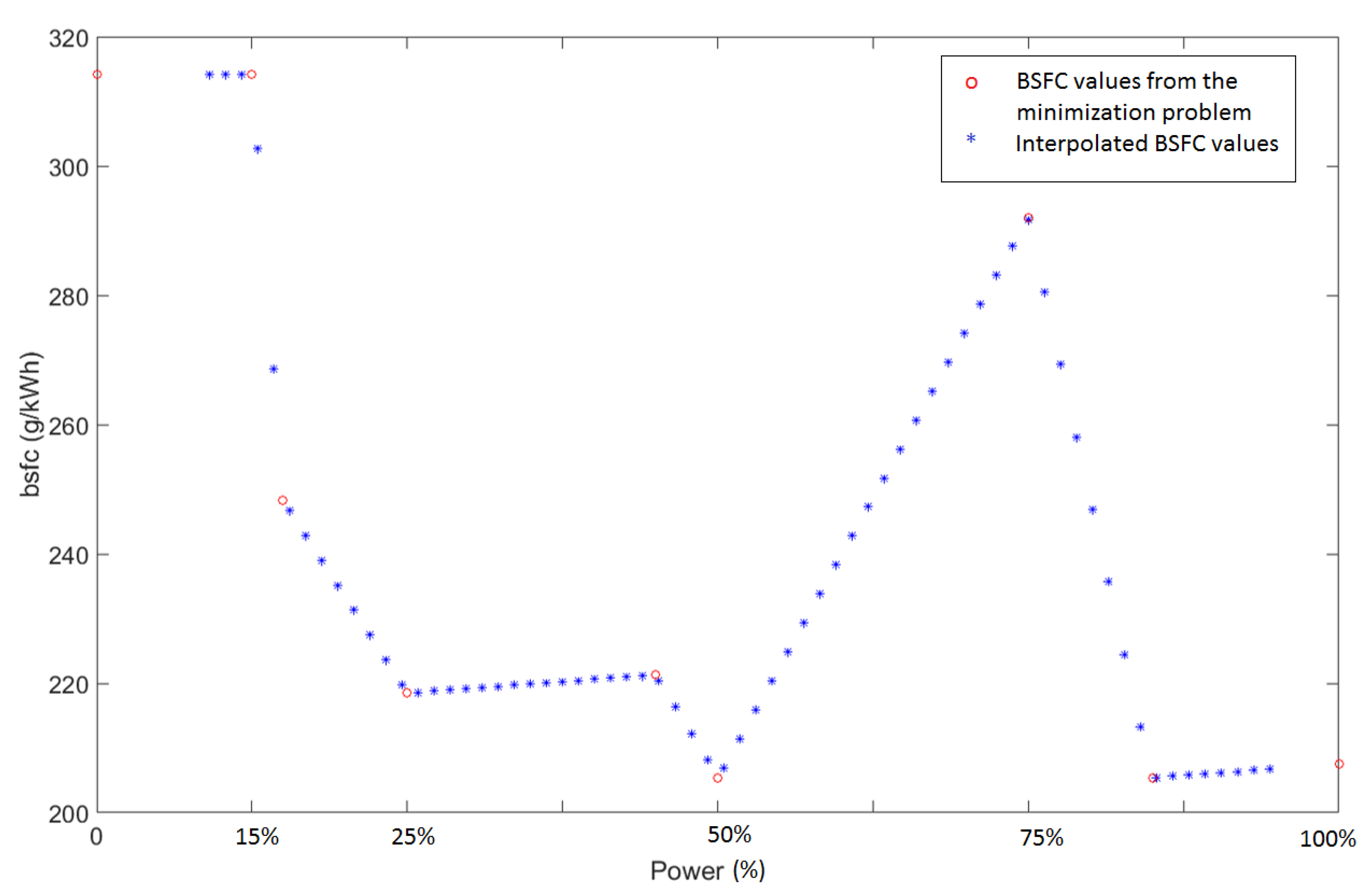
- BSFC(i) is the values calculated from Step 4 (as in Figure 6) (in g/kWh)
- Power(i) is the corresponding load (in kW)
- Time Percent(i) is the running time percentage of the corresponding load (in percent)
- Total Working Time is total running time in a working cycle (in hours)
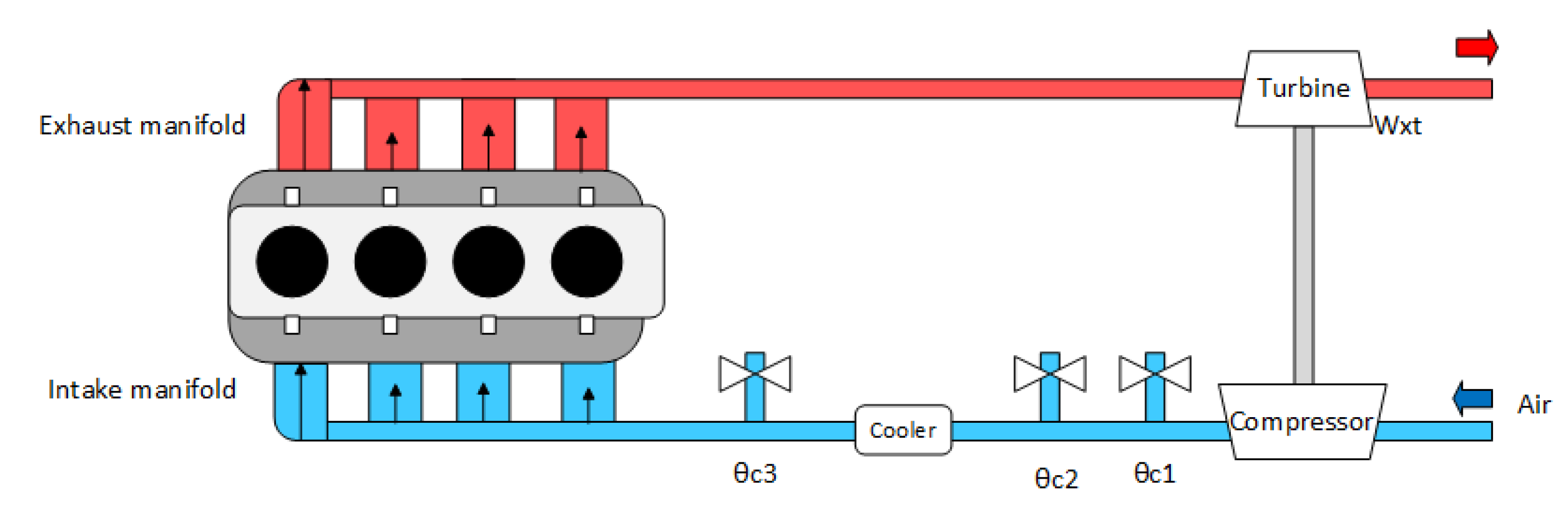
3.2. Experimental Apparatus
4. Results and Analysis
4.1. Results
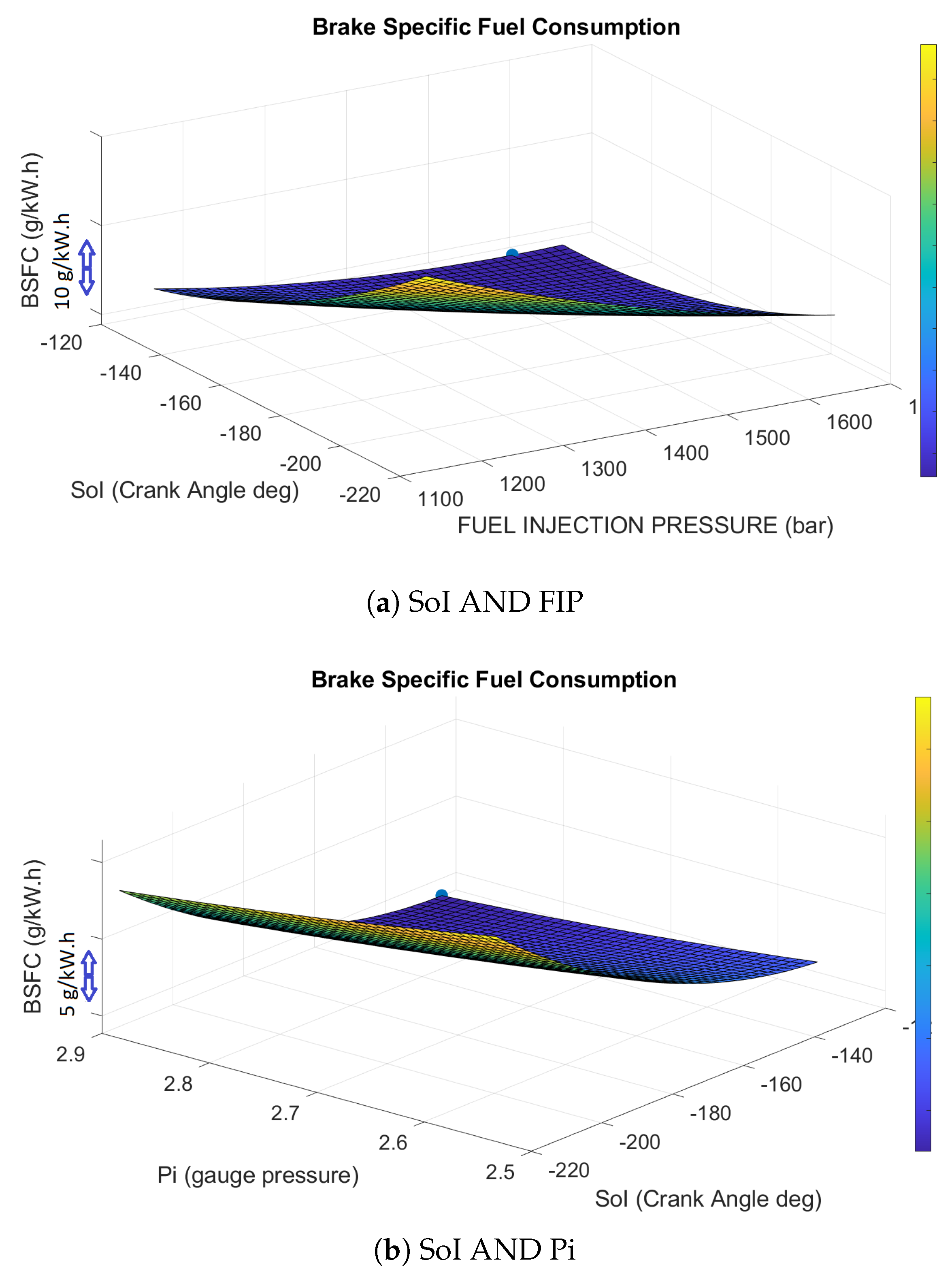
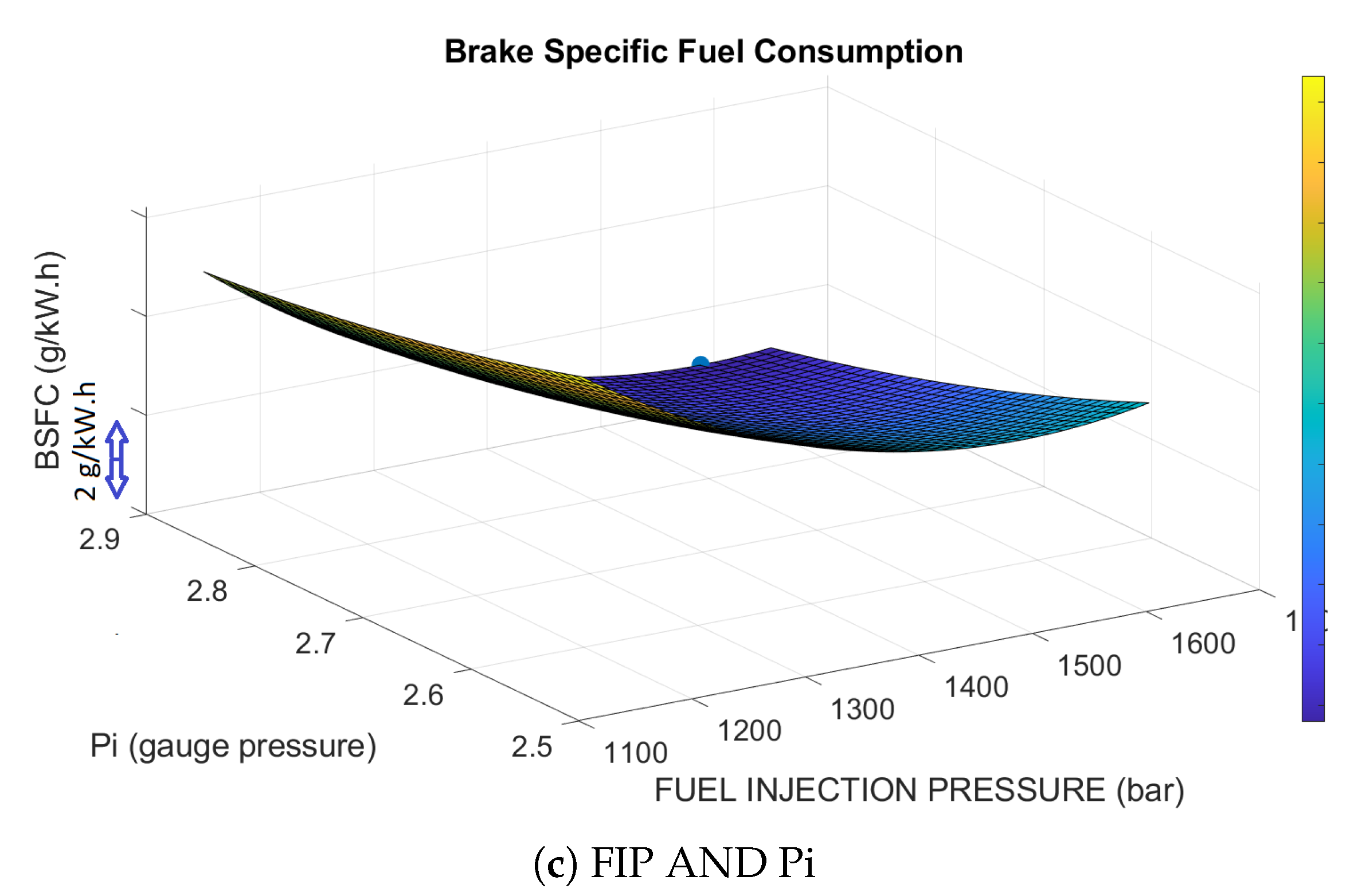
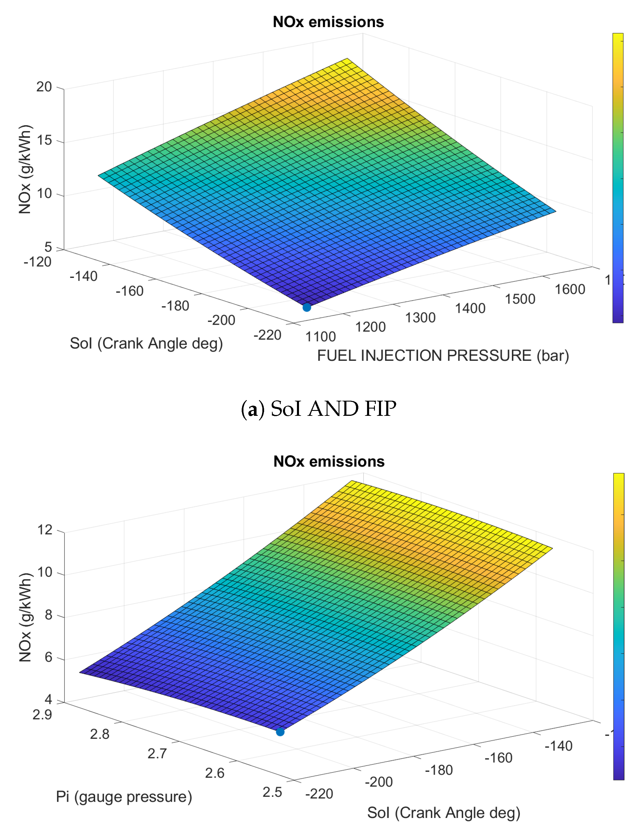
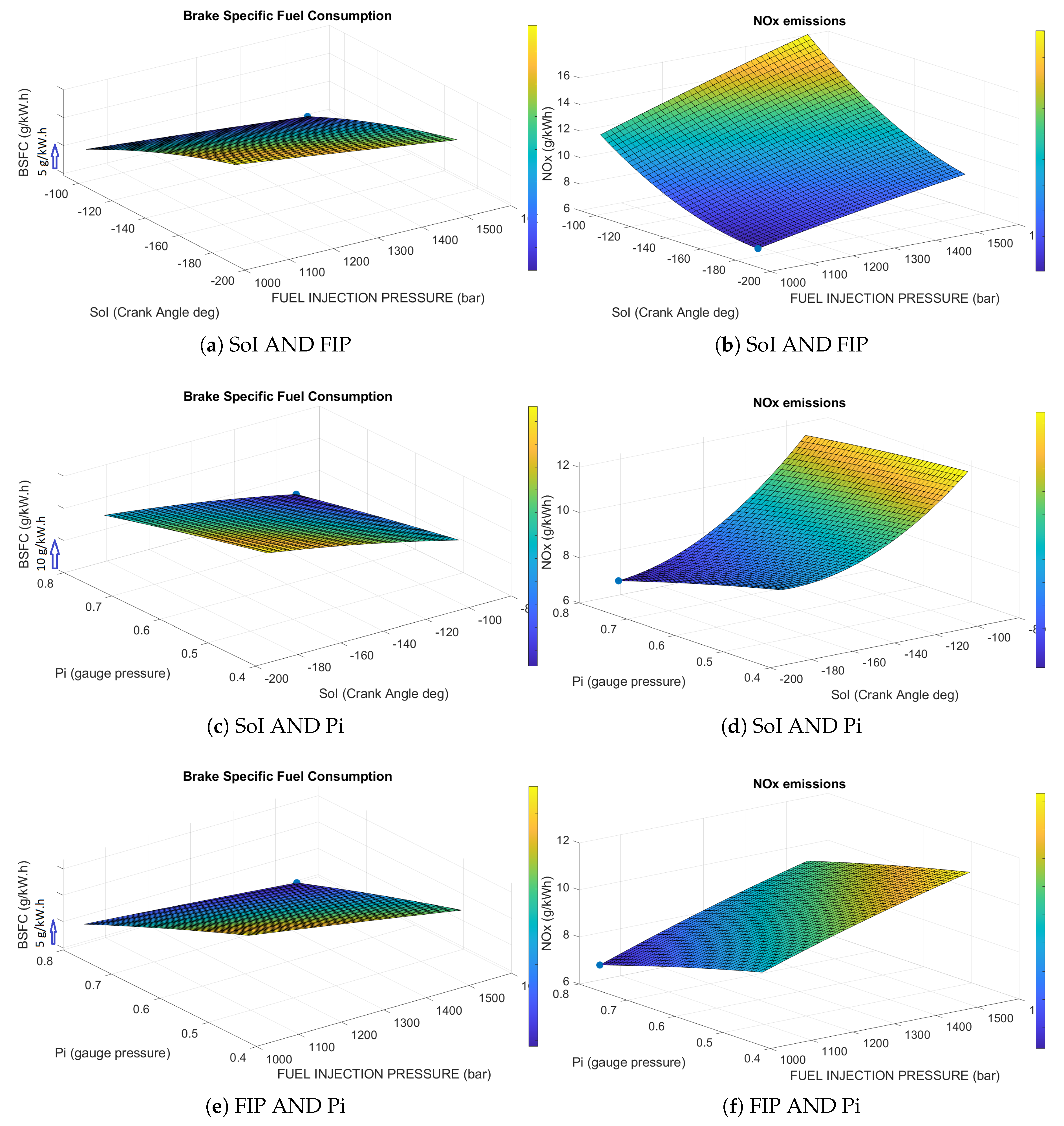
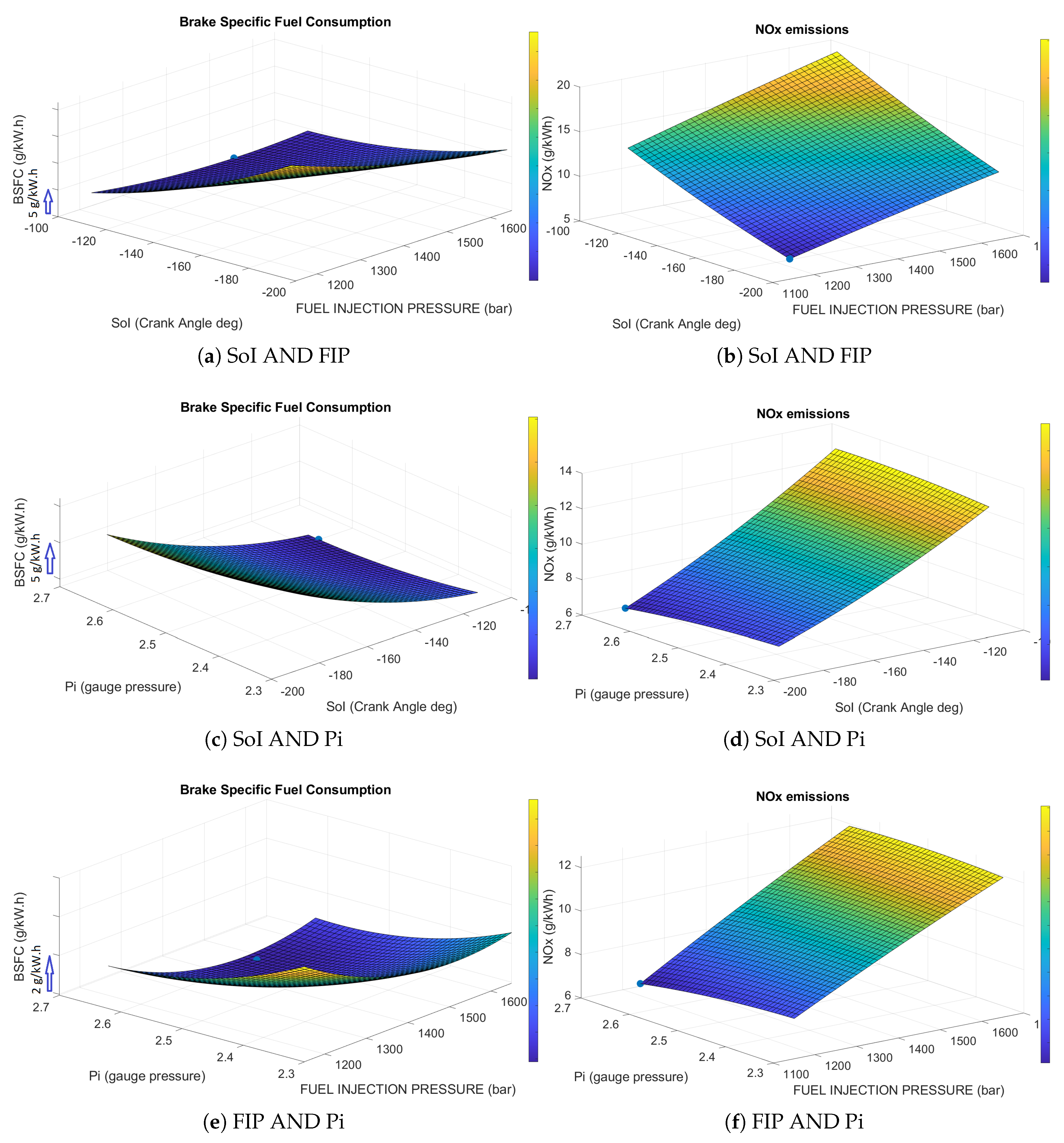
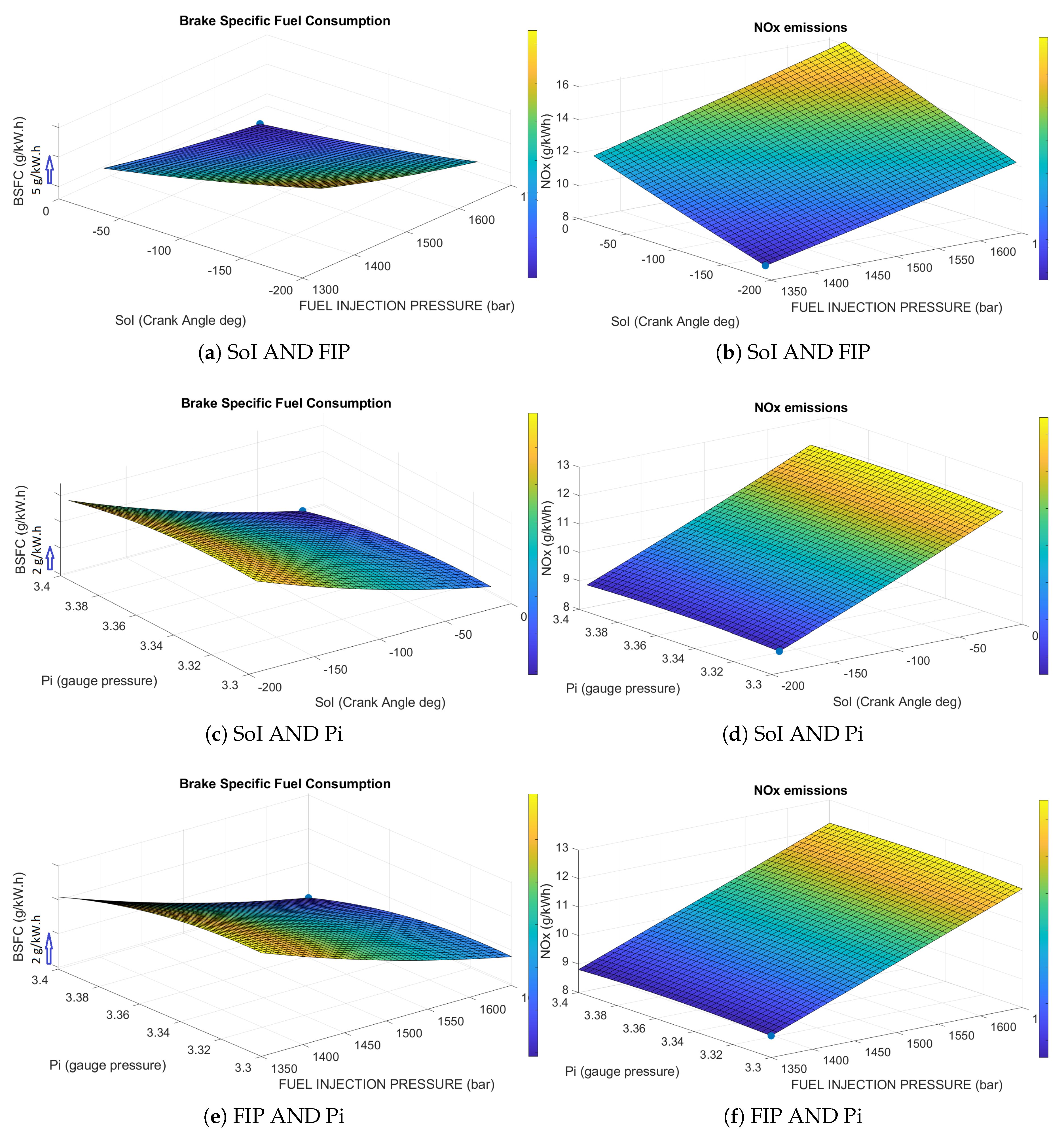
4.1.1. Modeling Results
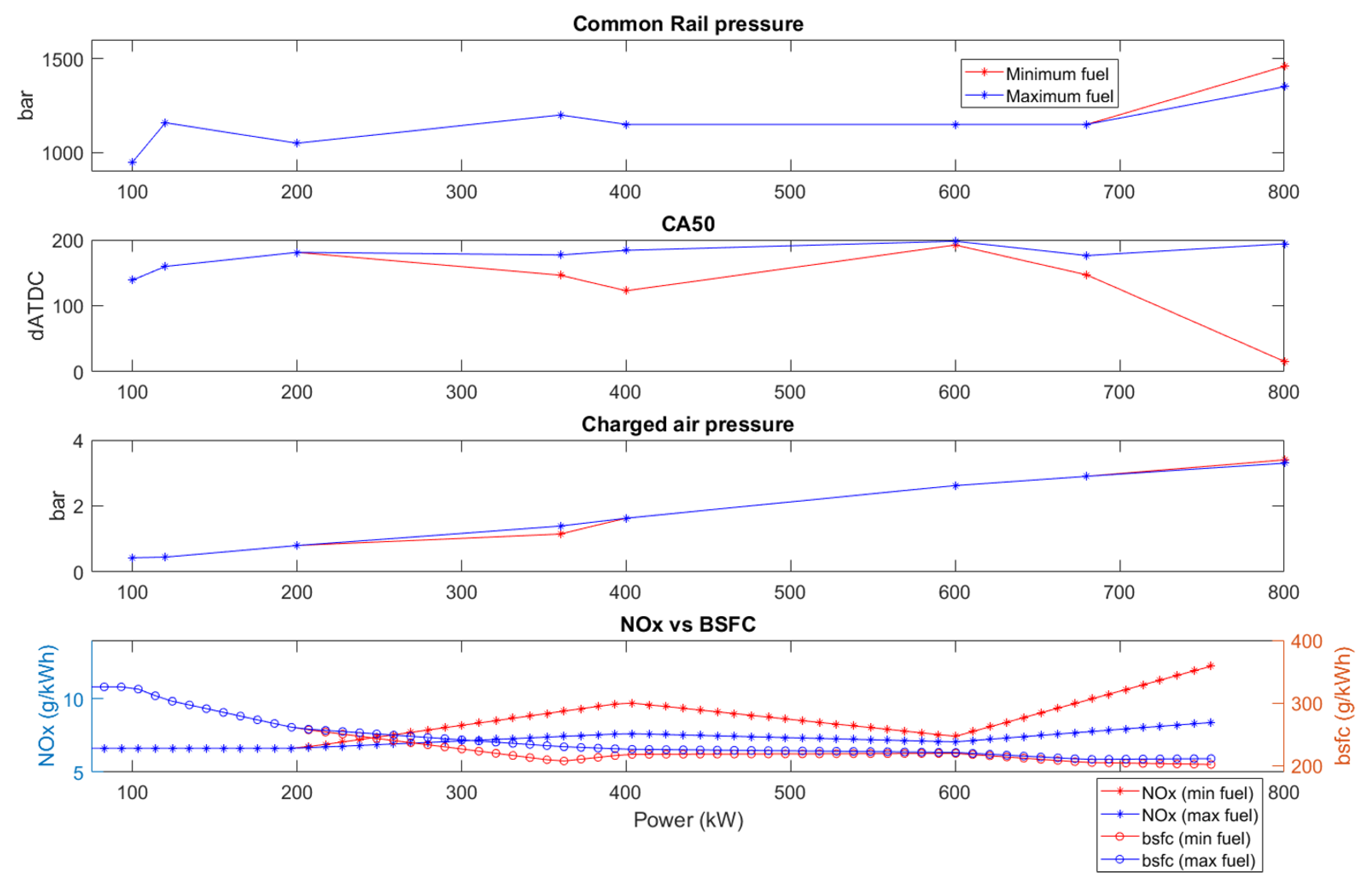
4.1.2. Optimization Results
4.2. Analysis
5. Discussion
- (1)
- First of all, the models of the BSFC and the can be improved by having more input parameters such as speed and load of the engine so that errors in the interpolation process of the BSFC can be avoided.
- (2)
- Secondly, in STEP 1 and STEP 2 of the algorithm, the value of k can be increased for higher accuracy but it requires more computational effort and resources. Furthermore, the functions could be made as continuous functions instead of discrete functions.
- (3)
- As the value of k increases, the number of possible lines increases exponentially and more appropriate conditions should be applied alongside the IMO Tier II condition in (1). For instance, by using the fact that the BSFC and the emissions have a direct trade-off, if the BSFC needs to be minimized then only maximum eligible lines are taken. Hence, by reducing the number of eligible lines, less computation will be needed.
- (4)
- It should be noticed that to reduce the total amount of fuel used, the total amount of emitted is slightly increased although the limits according to the IMO Tier II are still fulfilled. This fact shows the lack of coverage of the emission legislation. Due to this, different optimization strategies have a big difference in the total emitted, as long as the limits are satisfied.
- (5)
- Last but not least, it would be better to include more physical constraints to the optimization algorithm rather than only the emissions constraint. The thermal load of the engine, the soot limit or the emissions would make the optimizer become more sufficient.
6. Conclusions
- (1)
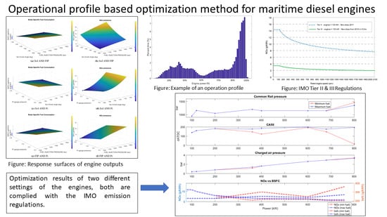
- The optimization method has been proven to be capable of saving fuel consumption and fulfilling the IMO Tier II emission regulation (E2 test cycle in particular).
- (2)
- Using operational profile for optimizing the fuel consumption creates more possibilities to calibrate the engines according to their working cycles. Flexible settings are needed for the engines to operate in different conditions and applications.
- (3)
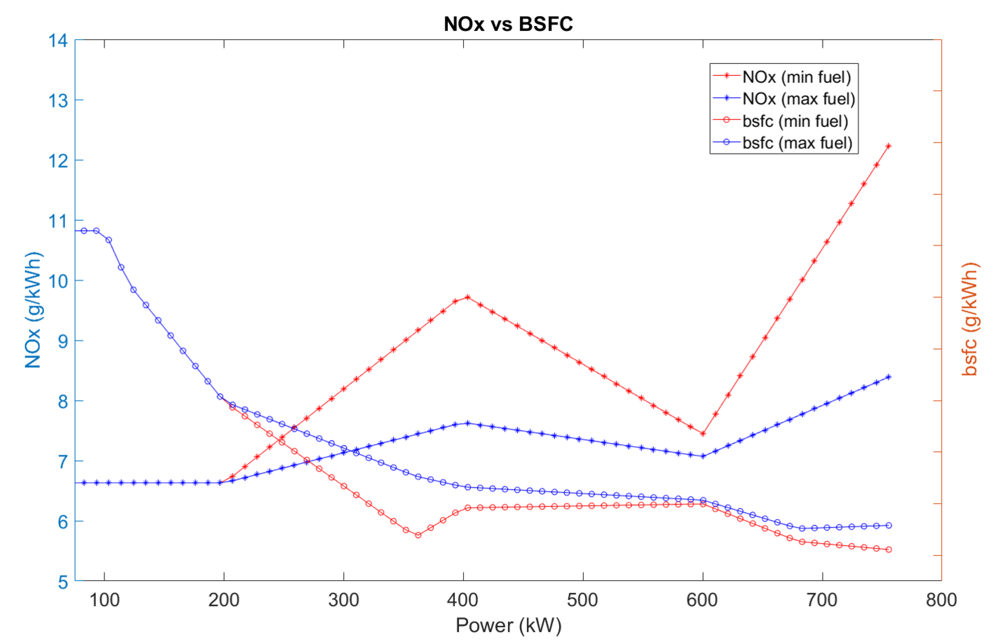
- By using different constraints (different lines), the total fuel consumption can be optimized to serve different purposes while the IMO Tier II is still fulfilled. In Table 5, the difference between the minimum and the maximum fuel consumption during a working cycle of 5000 h is around 17 tons (approximately 3.1%) while the according produced difference is around 25%. This shows a lot of opportunities for the engine calibration to balance the trade-off between the BSFC and the emissions.
Author Contributions
Funding
Conflicts of Interest
Abbreviations
| BSFC | Brake Specific Fuel Consumption |
| IMO | International Maritime Organization |
| Nitrogen Oxides | |
| FIP | Fuel Injection Pressure |
| SoI | Start of Injection |
| DoE | Design of Experiments |
| RSM | Response Surface Methods |
| FSHP | Folding, Shrinking Hyper Parallelepiped |
Appendix A


References
- Montgomery, D.; Reitz, R.D. Six-mode cycle evaluation of the effect of EGR and multiple injections on particulate and NOx emissions from a DI diesel engine. SAE Trans. 1996, 105, 356–373. [Google Scholar]
- Rao, S.; Desai, R. Optimization theory and applications. IEEE Trans. Syst. Man Cybern. 1980, 10, 280. [Google Scholar] [CrossRef]
- Lenz, U.; Schroeder, D. Artificial Intelligence for Combustion Engine Control; Technical Report, SAE Technical Paper 960328; SAE International: Warrendale, PA, USA, 1996. [Google Scholar]
- Tsao, G.M.; Chang, T.; Tsao, K. An Expert System Based Approach to Internal Combustion Engine Experimentation; Technical Report, SAE Technical Paper 910052; SAE International: Warrendale, PA, USA, 1991. [Google Scholar]
- Pilley, A.; Beaumont, A.; Robinson, D.; Mowll, D. Design of experiments for optimization of engines to meet future emissions targets. In Proceedings of the 27th International Symposium on Automotive Technology and Automation, Aachen, Germany, 31 October–4 November 1994. [Google Scholar]
- Edwards, S.P.; Pilley, A.; Michon, S.; Fournier, G. The Optimisation of Common Rail FIE Equipped Engines Through the Use of Statistical Experimental Design, Mathematical Modelling and Genetic Algorithms. SAE Trans. 1997, 106, 505–523. [Google Scholar]
- Montgomery, D.; Reitz, R. Applying design of experiments to the optimization of heavy-duty diesel engine operating parameters. In Statistics for Engine Optimization; Edwards, S., Grove, D., Wynn, H., Eds.; Professional Engineering Publishing Ltd.: London, UK, 2000. [Google Scholar]
- Toyoda, M.; Shen, T. D-optimization based mapping calibration of air mass flow in combustion engines. In Proceedings of the 2016 European Control Conference (ECC), Aalborg, Denmark, 29 June–1 July 2016; pp. 1259–1264. [Google Scholar]
- Langouët, H.; Métivier, L.; Sinoquet, D.; Tran, Q.H. Engine calibration: Multi-objective constrained optimization of engine maps. Optim. Eng. 2011, 12, 407–424. [Google Scholar] [CrossRef]
- Montgomery, D.T.; Reitz, R.D. Optimization of heavy-duty diesel engine operating parameters using a response surface method. SAE Trans. 2000, 109, 1753–1765. [Google Scholar]
- Baldi, F.; Larsen, U.; Gabrielii, C. Comparison of different procedures for the optimisation of a combined Diesel engine and organic Rankine cycle system based on ship operational profile. Ocean Eng. 2015, 110, 85–93. [Google Scholar] [CrossRef]
- Knafl, A.; Stiesch, G.; Friebe, M. Optimal utilization of air- and fuel-path flexibility in medium-Speed diesel engines to achieve superior Performance and fuel Efficiency. In Proceedings of the 27th CIMAC World Congress on Combustion Engine Technology, Shanghai, China, 13–16 May 2013. [Google Scholar]
- Khac, H.N.; Zenger, K. Designing optimal control maps for diesel engines for high efficiency and emission reduction. In Proceedings of the 2019 18th European Control Conference (ECC), Naples, Italy, 25–28 June 2019; pp. 1957–1962. [Google Scholar] [CrossRef]
- Abdullah, N.R.; Shahruddin, N.S.; Mamat, R.; Ihsan Mamat, A.; Zulkifli, A. Effects of air intake pressure on the engine performance, fuel economy and exhaust emissions of a small gasoline engine. J. Mech. Eng. Sci. 2014, 6, 949–958. [Google Scholar] [CrossRef]
- Richard, S. Introduction to Internal Combustion Engines; Palgrave Macmillan: London, UK, 2012. [Google Scholar]
- Xu, Z.; Li, X.; Guan, C.; Huang, Z. Effects of injection pressure on diesel engine particle physico-chemical properties. Aerosol Sci. Technol. 2014, 48, 128–138. [Google Scholar] [CrossRef]
- Jayashankara, B.; Ganesan, V. Effect of fuel injection timing and intake pressure on the performance of a DI diesel engine—A parametric study using CFD. Energy Convers. Manag. 2010, 51, 1835–1848. [Google Scholar] [CrossRef]
- VI, R.M.A. Regulations for the Prevention of Air Pollution from Ships and NOX Technical Code 2008; International Maritime Organization: London, UK, 2009. [Google Scholar]
- Mathews, P.G. Design of Experiments with MINITAB; ASQ Quality Press: Milwaukee, WI, USA, 2005. [Google Scholar]
- Boggs, P.T.; Tolle, J.W. Sequential quadratic programming. Acta Numer. 1995, 4, 1–51. [Google Scholar] [CrossRef]


| Speed (%) | 100 | 100 | 100 | 100 |
| Power (%) | 25 | 50 | 75 | 100 |
| Weighting factor | 0.15 | 0.15 | 0.5 | 0.2 |
| Cylinder number | 4 |
| Cylinder bore | 200 mm |
| Piston stroke | 280 mm |
| Swept volume | 0.0088 |
| Rated speed | 1000 rpm |
| Rated power | 800 kW |
| Parameters | Devices |
|---|---|
| Eco Physics CLD 822 M hr | |
| CO, | Siemens Ultramat 6 |
| Hydrocarbons | J.U.M.VE7 |
| Cylinder pressure | Kistler KiBox |
| Injection timing | Current probe |
| Fuel consumption | HBM weight cell, Sartorius X3 |
| Speed (rpm) | 1000 | 900 | 800 | 700 | 600 | |
|---|---|---|---|---|---|---|
| Load (kW) | ||||||
| 100 kW | ✓ | ✓ | ✓ | ✓ | ||
| 150 kW | ✓ | |||||
| 200 kW | ✓ | ✓ | ✓ | ✓ | ||
| 300 kW | ✓ | |||||
| 400 kW | ✓ | ✓ | ||||
| 600 kW | ✓ | |||||
| 800 kW | ✓ | |||||
| Yearly fuel consumption (tons) | ||
| Minimum Fuel | Maximum Fuel | Percentage |
| Case | Case | (Min-Max) |
| 550.9 | 567.3 | −3.1% |
| Yearly produced (tons) | ||
| Minimum Fuel | Maximum Fuel | Percentage |
| Case | Case | (Min-Max) |
| 24.7 | 19.7 | 25.4% |
© 2020 by the authors. Licensee MDPI, Basel, Switzerland. This article is an open access article distributed under the terms and conditions of the Creative Commons Attribution (CC BY) license (http://creativecommons.org/licenses/by/4.0/).
Share and Cite
Nguyen Khac, H.; Zenger, K.; Storm, X.; Hyvönen, J. Operational Profile Based Optimization Method for Maritime Diesel Engines. Energies 2020, 13, 2575. https://doi.org/10.3390/en13102575
Nguyen Khac H, Zenger K, Storm X, Hyvönen J. Operational Profile Based Optimization Method for Maritime Diesel Engines. Energies. 2020; 13(10):2575. https://doi.org/10.3390/en13102575
Chicago/Turabian StyleNguyen Khac, Hoang, Kai Zenger, Xiaoguo Storm, and Jari Hyvönen. 2020. "Operational Profile Based Optimization Method for Maritime Diesel Engines" Energies 13, no. 10: 2575. https://doi.org/10.3390/en13102575
APA StyleNguyen Khac, H., Zenger, K., Storm, X., & Hyvönen, J. (2020). Operational Profile Based Optimization Method for Maritime Diesel Engines. Energies, 13(10), 2575. https://doi.org/10.3390/en13102575