Abnormality Detection of Cast-Resin Transformers Using the Fuzzy Logic Clustering Decision Tree

Abstract

Failures of cast-resin transformers not only reduce the reliability of power systems, but also have great effects on power quality. Partial discharges (PD) occurring in epoxy resin insulators of high-voltage electrical equipment will result in harmful effects on insulation and can cause power system blackouts. Pattern recognition of PD is a useful tool for improving the reliability of high-voltage electrical equipment. In this work, a fuzzy logic clustering decision tree (FLCDT) is proposed to diagnose the PD concerning the abnormal defects of cast-resin transformers. The FLCDT integrates a hierarchical clustering scheme with the decision tree. The hierarchical clustering scheme uses splitting attributes to divide the data set into suspended clusters according to separation matrices. The hierarchical clustering scheme is regarded as a preprocessing stage for classification using a decision tree. The whole data set is divided by the hierarchical clustering scheme into some suspended clusters, and the patterns in each suspended cluster are classified by the decision tree. The FLCDT was successfully adopted to classify the aberrant PD of cast-resin transformers. Classification results of FLCDT were compared with two software packages, See5 and CART. The FLCDT performed much better than the CART and See5 in terms of classification precisions.

1. Introduction

The power transformer is an important equipment in a power system, which directly affects the safety of the power station and the safe operation of the power grid. Among them, the cast-resin transformer provides the products numerous excellent characters such as low no-load loss, oilless, anti-flaming, maintenance-free, good moisture resistance and crazing resistance, etc. The cast-resin transformer is perfectly matched to the requirement on inflammable and explosive site such as commercial center, high-tech factory, hospital, underground, airport, train station, tower building, industrial and mining enterprise, etc. Disturbances of power quality will result in significant financial consequences to network operators and customers. Since many uncertainties are involved, it is difficult to obtain exact financial losses due to poor power quality. Therefore, online monitoring of the cast-resin transformers has been an important challenge for power engineers. Failures of cast-resin transformers not only reduce reliability of power system, but also have great effects on power quality. Power engineers are devoted to intensifying diagnosis on the cast-resin transformer for discovering hidden troubles timely and guaranteeing the normal operation of the cast-resin transformer. Partial discharge (PD) is one of the main causes which leads to internal insulation deterioration of the cast-resin transformer. Online monitoring of PD can reduce the risk of insulation failure of cast-resin transformers [1]. There are many methods, such as ultrasound, acoustic emission, electrical contact, optical and radio frequency sensing, could be used to detect and locate PD in a cast-resin transformer [2]. For electrical detection, UHF antenna is widely used in the PD measurements because it is more sensitive than other methods with regard to the noise issue.

PD is a localized electrical discharge that occurs repetitively in a small region. In general, PD can be categorized into six forms from their occurring causes: corona discharge, surface discharge, internal discharge, electrical tree, floating partial discharge and contact noise. Corona discharge takes place at atmospheric pressure in the presence of inhomogeneous fields. Surface discharge appears in arrangements with tangential field distribution along the boundary of two different insulation materials. Internal discharge occurs within cavities or voids inside solid or liquid dielectrics. Electric trees occur at points where gas voids, impurities, mechanical defects or conducting projections cause excessive local electrical field stresses within small regions of the dielectric. Floating PD occurs when there is an ungrounded conductor within the electric field between conductor and ground. Contact noise occurs if the ground connection to a bushing is poor.

PD occurs in high-voltage electrical equipment, such as cables, transformers, motors and generators. It is a kind of very small spark that occurs due to a high electrical field. Since a PD occurring in high-voltage electrical equipment has a specific pattern, pattern recognition of PD is a useful tool for improving the reliability of high-voltage electrical equipment [3]. With the development of electricity, the PD diagnosis is a useful tool for evaluation of the cast-resin transformer and prevention of the possible failures. It is essential to determine the different types of faults by PD diagnosis to estimate the likely defect type and severity. The use of PD pattern recognition can identify potential faults and inspect insulation defects from the measured data. Then, the potential effects are used to estimate the risk of insulation failure in high-voltage electrical equipment. This information is important to evaluate the risk of discharge in the insulation. PD pattern recognition in the past depended on expert judgments for classification and defect level determination. Such a process is unscientific and needs professional experience from years’ practice.

To date, artificial intelligent techniques were adopted for pattern recognition and classification of PD. Mor et al. used the cross wavelet transform to perform automatic PD recognition [4]. The wavelet analysis has been regarded as a promising tool to denoising and fault diagnosis, however it is difficult to determine the composition level that yields the best result. Gu et al. proposed a fractional Fourier transform-based approach for gas-insulated switchgear PD recognition [5]. Ma et al. proposed a fractal theory-based PD recognition technique for medium-voltage motors [6]. However, some clusters of PD patterns are very close in the fractal map, which may result in incorrect identification.

As a more scientific approach, machine learning technique for PD recognition is utilized to bypass human errors [7].

There exist numerous machine learning techniques for the pattern recognition of PD such as the artificial neural network [8], clustering [9,10], support vector machine [11] and deep learning [12,13,14]. The artificial neural network constitutes an information processing model which contains empirical knowledge using a learning process. However, it is computationally expensive and lack of rules for determining the proper network structure. The clustering technique is set up based on the stream density and the clustering theory, however the zero-weight problem exists in the general clustering approach. The support vector machines belong to supervised learning techniques based on statistical learning theory which may be applied for PD pattern recognition, however the classification performance of SVM is conveniently affected by the setting of parameters. Deep learning was successfully applied in pattern recognition and image segmentation, however it is a challenging task due to the limited data availability.

The contribution of this work is to develop a fuzzy logic clustering decision tree (FLCDT) to classify the abnormal defects of cast-resin transformers. Fuzzy logic methods have been successfully applied to many applications in renewable energy. Liu et al. developed an ultra-short-time forecasting method based on the Takagi–Sugeno fuzzy model for wind power and wind speed [15]. In [16], an offline time series forecasting approach with an adaptive neuro-fuzzy inference system was conducted for electrical insulator fault forecast. Wang et al. proposed a fuzzy hybrid model to evaluate the energy policies and investments in renewable energy resources [17]. Thao et al. presented an improved interval fuzzy modeling technique to estimate solar photovoltaic, wind and battery power in a demonstrative renewable energy system under large data changes [18].

A 60-MVA cast resin transformer with a rated voltage of 22.8 kV is used in this study. The IEC 60,270 standard [19] is utilized to perform an off-line PD measurement on electrical equipment. The training dataset has three continuous attributes and three abnormal defects. 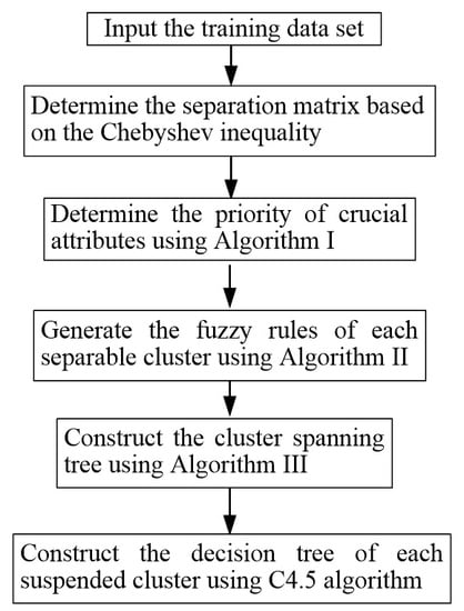Three continuous attributes are the number of discharge (n) over the chosen block, discharge magnitude (q) and the corresponding phase angle ($\varphi$) where PD pulses occur. Three abnormal defects are failure in S-phase cable termination, failure in R-phase cable and failure in T-phase cable termination. The FLCDT integrates a hierarchical clustering scheme with the decision tree. The hierarchical clustering scheme uses splitting attributes to divide the data set into suspended clusters according to a separation matrix and fuzzy rules. The suspended clusters consist of more than one pattern, which can be further classified by the decision tree [20].

In the remaining part of the study, the Section 2 is used to present the fuzzy logic clustering decision tree. Section 3 introduces the PD measurements of cast-resin transformers and describes the pattern recognition of PD. In Section 4, the FLCDT is applied to classify the aberrant PD of cast-resin transformers and compared with two software packages, See5 and CART. Finally, Section 5 makes a conclusion.

2. The Fuzzy Logic Clustering Decision Tree

2.1. Motivation

Since the number of possible attributes and the number of classes are rather large, data mining techniques have been receiving increasing attention from the research community. For example, the fault detection of the ion implantation processes is a challenging issue in semiconductor fabrication because of the large number of wafer recipes. Fuzzy-rule-based classification algorithms [21,22] have received significant attention among researchers due to a finer fuzzy partition and good behavior in the real-time databases. These advantages may be suppressed if the number of attributes and number of classes become large, a finer partition of fuzzy subsets is required and results in a large size of the fuzzy-rule sets. To resolve this disadvantage, the main characteristic of the developed method is to divide the classes into specific clusters to accomplish a finer partition of fuzzy subsets. Figure 1 illustrates an eight-class example of cluster splitting, which is divided into four suspended clusters. In each cluster, the recognizability now is four times larger than the original structure. Thus, the approach not only can achieve higher classification accuracy, but also spend less computational complexity.

Since the cluster can be further classified by data mining techniques, the concept of clustering of the proposed method is hierarchical. The hierarchical concept had been adopted fairly widely in various classification methods, including the hierarchical decision trees [23,24], hierarchical Bayesian networks [25,26] and hierarchical neural networks [27,28], to improve the computation time and accuracy of classification. Accordingly, the FLCDT scheme is proposed to achieve a finer fuzzy partition without expensive computation. The motivation of the FLCDT is to measure the distance between two classes of an attribute. A separability factor is used to decide whether the two classes belong to the same cluster or not. After performing the FLCDT, a cluster spanning tree containing a cluster leader and some suspended clusters will be constructed. A cluster leader is the root of the cluster spanning tree. The classes in any suspended cluster is much less than the cluster leader. The flow diagram of the FLCDT scheme is displayed in Figure 2.

2.2. Splitting Cluster

2.2.1. Separation Matrix Based on the Chebyshev Inequality

Since not all the attributes are indispensable to separate classes, a specified criterion can be used to select few critical and effective ones to split clusters. The attribute values for members in the given training data spread over a specific range with a particular probability density function. Thus, the overlapping degree of the attribute values is used to decide the separability between two classes. For instances, Figure 3 shows two classes $C_i$ and $C_j$ for the kth attribute are separable, while Figure 4 shows two classes are not separable.

The separability factor is used to determine whether two classes $C_i$ and $C_j$ for the $k$th attribute are separable or not, which is defined as

$$S{(C_i,C_j)}_k=\{\begin{array}{cc}0,\hfill & \mathrm{if}{C}_i\mathrm{and}{C}_j\mathrm{are}\mathrm{separable}\mathrm{for}\mathrm{the}k\mathrm{th}\mathrm{attribute},\hfill \\ 1,\hfill & \mathrm{otherwise}.\hfill \end{array}$$

(1)

The value of $S{(C_i,C_j)}_k$ is calculated by the Chebyshev inequality [29]. Let $X_i^k$ denote the random variable for the $k$th attribute of class $C_i$. We assume without loss of generality that ${\mu }_i^k<{\mu }_j^k$, where ${\mu }_i^k$ and ${\sigma }_i^k$ represent the mean and standard deviation of $X_i^k$, respectively. Let $a_i^k$ be a positive real value such that $\mathrm{P}\left(\left|X_i^k-{\mu }_i^k\right|\ge a_i^k\right)\le \alpha$, where $P[(\cdot )]$ represents the probability of $(\cdot )$, and $\alpha$ denotes the significance level, which is set to be 0.05. Based on the Chebyshev inequality [29], the value of $a_i^k$ is set as $\frac{{\sigma }_i^k}{\sqrt{0.05}}$. Once $a_i^k$ is obtained, an upper-bound, ${\overline{p}}_i=\min \left(1{,}_{}{\left[{\sigma }_i^k/\max (\delta ,{\mu }_j^k-{\mu }_i^k-a_i^k)\right]}^2\right)$, is determined according to the Chebyshev inequality such that $P\left(|X_j^k-{\mu }_j^k|\ge \max (\delta ,{\mu }_j^k-{\mu }_i^k-a_i^k)\right)\le {\overline{p}}_i$, where $\delta$ is a tiny positive real value. If ${\mu }_j^k$ is sufficiently greater than ${\mu }_i^k+a_i^k$, the value of ${\overline{p}}_i$ is very small, two classes $C_i$ and $C_j$ are more easily separable as illustrated in Figure 5. Thus, a threshold value $\widehat{p}$ can be used to determine the separation factor for two classes $C_i$ and $C_j$.

$$S{(C_i,C_j)}_k=\{\begin{array}{c}\begin{array}{ccc}0,\hfill & if\hfill & {\overline{p}}_i<\widehat{p}\hfill \end{array},\hfill \\ \begin{array}{cc}1,\hfill & \mathrm{otherwise}.\hfill \end{array}\hfill \end{array}$$

(2)

Now, the separation matrix for the $k$th attribute is defined as $[S{(C_i,C_j)}_k]$, whose ($i,j$)th element is $S{(C_i,C_j)}_k$.

2.2.2. Divide Cluster

To select the classes which are belong to a same cluster, a separability graph according to the separability matrix $[S{(C_i,C_j)}_k]$ is constructed. Regarding a class as a node, $[S{(C_i,C_j)}_k]$ is treated as an incidence matrix of the kth attribute. If $S{(C_i,C_j)}_k=1$, two nodes $C_i$ and $C_j$ are connected by an arc. The separability graph contains several disjoint connectivity sub-graphs. A connectivity sub-graph indicates a cluster, and the amount of disjoint connectivity sub-graphs is the number of suspended clusters which are obtained by the $k$th attribute. For example, Figure 6 shows a separability graph, which is constructed according to the separability matrix shown in Figure 7. The separability graph has two clusters, the first one comprises classes 1, 2, 3 and 4, and the other comprises classes 5, 6, 7 and 8.

2.3. Selection of Crucial Attributes

It is possible that all classes are not separable using an attribute. The separability graph may be a connectivity graph using this attribute. Thus, an attribute which can divide all classes into at least two clusters is defined as a crucial attribute (CA). Since there are several CAs in the training data, a disjoint cluster obtained using some CA can be further divide using other CA. This is the reason that we claim the proposed cluster splitting is a hierarchical cluster splitting. Because the priority of CAs utilized to split the classes will influence the classification accuracy, we describe the procedures of the hierarchical cluster splitting as below. First, the set of overall classes is defined as the cluster leader ${Cr}_0$. After successively applying two CAs, say CA${}_1$ and CA${}_2$, to ${Cr}_0$, the connectivity is resulted from the conjunction operation of $[S{(C_i,C_j)}_{k_1}]$ and $[S{(C_i,C_j)}_{k_2}]$, where $k_1$ and $k_2$ represent the selecting attribute of CA${}_1$ and CA${}_2$, respectively. The conjunction operation of two matrices is defined as the $(i,j)$th entry of $[S{(C_i,C_j)}_{k_1}]\wedge [S{(C_i,C_j)}_{k_2}]$ is performed by Boolean algebra, $S{(C_i,C_j)}_{k_1}\wedge S{(C_i,C_j)}_{k_2}$. Figure 8 displays a typical cluster spanning tree of $m$ CAs, where $C{A}_i$ represents the CA used in the ith level, L is the number of clusters in the first level, and n_L denotes the number of clusters in the second level of the cluster C_L. The suspended cluster (SC) is a cluster obtained from the last CA in the CA priority sequence or contains only one class.

For any priority sequence of CAs, the number of SCs in the cluster spanning tree are the same. However, an improper splitting of former clusters will affect the accuracy of the latter cluster splitting along the path of cluster spanning tree. For example, Figure 9 and Figure 10 show the separability matrices of a classification problem with 8 classes, C₁~C₈ and two attributes, $k_1$ and $k_2$. If the $k_1$ attribute is used first to split the 8 classes in Figure 9, there are three clusters after splitting. One comprises 1 class, and the other two comprise 3 and 4 classes. If the $k_2$ attribute is used first to split the 8 classes in Figure 10, there are four clusters after splitting and each cluster contain 2 classes. The $k_2$ attribute is chosen to split the cluster leader because it results in more SCs.

To describe the criterion, we define $L_k$ and $n_{k,l}(C{r}_j)$ as the amount of SCs and the amount of classes in the $l$th SC obtained by the $k$th attribute to divide the cluster $C{r}_j$, respectively. The criterion for selecting the attribute $k$ to divide $C{r}_j$ is

$${\min }_{}{\upsilon }_k(C{r}_j)=\frac{1}{L_k}\times \left(\left[{\displaystyle \sum _{l=1}^{L_k}{\left(n_{k,l}(C{r}_j)-{\overline{n}}_{k,l}\left(C{r}_j\right)\right)}^2}/(L_k-1)\right]+1\right)$$

(3)

where ${\overline{n}}_{k,l}\left(C{r}_j\right)={\displaystyle \sum _{l=1}^{L_k}{n}_{k,l}\left(C{r}_j\right)}/L_k$ is the average amount of classes in the obtained SCs. Obviously, the attribute will result in more SCs if it has a smaller variation concerning the number of classes in the SCs. This attribute is the CA that we seek. Consider the separability matrices shown in Figure 9 and Figure 10, if the $k_1$ attribute is used to divide the cluster first, there are three SCs. One comprises one class the other two comprise three and four classes. The value of ${\upsilon }_{k_1}\left(C{r}_0\right)$ is 1.11. If the $k_2$ attribute is used first, there are four SCs and each SC comprises two classes. The value of ${\upsilon }_{k_2}\left(C{r}_0\right)$ is 0.25. Since the value of ${\upsilon }_{k_2}\left(C{r}_0\right)$ is the smallest, the $k_2$ attribute is chosen to split $C{r}_0$.

Now, the algorithm (Algorithm 1) to determine the priority of CAs for constructing the cluster spanning tree is described below.

Algorithm 1: Determine the priority of CAs

Step 1: Use the training data set to calculate the separation matrix for each attribute. Configure the set of Non-Split Clusters (NSC) = {$C{r}_0$}. Step 2: Determine the splitting attribute $k$ according to equation (3) for each cluster in NSC, then use this attribute to divide the clusters and move these SCs into NSC. Step 3: Remove the clusters which was divided and those cannot be divided by any attribute. Step 4: If $NSC=\phi$, stop; else, go to Step 2.

2.4. The Hierarchical Clustering Scheme

The hierarchical clustering scheme has two phases: the training phase for generating the fuzzy logic rules and the classifying phase to classify a new data pattern. In the training phase, a data set with predetermined SCs is given. The fuzzy logic rules are generated according to the given data patterns. In the classifying phase, a fuzzy inference mechanism is utilized to classify an unknown data pattern according to the fuzzy logic rules.

2.4.1. The Fuzzy Rules Generation

Consider a given training data set for a non-SC cluster $C{r}_j$ in the cluster spanning tree, an attribute $k_i$ can split the cluster into SCs. The $g$ given data patterns for attribute $k_i$ are denoted as $x_{k_i}^p$, $p=1,\dots ,g$, with $M$ known SCs, $SC{r}_{j1},\dots ,SC{r}_{jM}$. These $g$ data patterns are trained to split the non-SC cluster $C{r}_j$. The fuzzy if-then rule [30,31] is defined as follows.

$R_i$: If $x_{k_i}^p$ is $A_i^{\mathrm{I}}$, then $x_{k_i}^p$ belongs to $SC{r}_{ji}$ with $C{F}_i^{\mathrm{I}}$, where $I$ denotes the amount of fuzzy subsets, $A_i^{\mathrm{I}}$ denotes the $i$th fuzzy subset, $i=1,\dots ,I$, $SC{r}_{ji}$ represents the consequent, which is one of the $M$ SCs and $C{F}_i^{\mathrm{I}}$ denotes the certainty grade of rule $R_i$.

Let ${\mu }_i(\cdot )$ represent the membership function of $(\cdot )$ with respect to the fuzzy subset $A_i^{\mathrm{I}}$. Therefore, ${\mu }_i(x_{k_i}^p)$ can be treated as a compatibility grade of $x_{k_i}^p$ corresponding to $A_i^{\mathrm{I}}$. Define

$${\beta }_{SC{r}_{jl}}(R_i)={\displaystyle \sum _{x_p\in SC{r}_{jl}}{\mu }_i(x_{k_i}^p)}$$

(4)

as the sum of compatibility grade for $SC{r}_{jl}$ corresponding to $A_i^{\mathrm{I}}$. The generation of fuzzy logic rules to split cluster $C{r}_j$ is summarized as follows.

The step-wise process of the Algorithm 2 is given below.

Algorithm 2: Generate the fuzzy rules

Step 1: Given the $g$ training data $x_{k_i}^p$, $p=1,\dots ,g$ and the splitting attribute $k_i$ for cluster $C{r}_j$ with $M$ known $SC{r}_{jm}$, $m=1,\dots ,M$ and set $i=1$. Step 2: Compute the sum of compatibility grade for $SC{r}_{jm}$, $m=1,\dots ,M$, by (4). Step 3: Determine the $SC{r}_{jx}$ with the maximum sum of compatibility grade $${\beta }_{SC{r}_{jx}}(R_i)=\max \{{\beta }_{SC{r}_{j1}}(R_i),\dots ,{\beta }_{SC{r}_{jM}}(R_i)\}$$ (5) Step 4: Calculate the certainty grade $C{F}_i$ of rule $R_i$ $$C{F}_i=\left({\beta }_{SC{r}_{ix}}(R_i)-\beta (R_i)\right)/{\displaystyle \sum _{m=1}^M{\beta }_{SC{r}_{jm}}(R_i)}$$ (6) where $\beta (R_i)={\displaystyle \sum _{SC{r}_{jm}\ne SC{r}_{jx}}{\beta }_{SC{r}_{jm}}(R_i)/(M-1)}$ denotes the mean of the sum of compatibility grade for the rest SCs corresponding to $A_i^{\mathrm{I}}$. Step 5: If $i=I$, then stop; else, set $i=i+1$ and go to Step 2.

The hierarchical clustering scheme (Algorithm 3) is summarized as follows.

Algorithm 3: Hierarchical clustering scheme

Step 0: Set the threshold value $\widehat{p}$. Step 1: Calculate ${\mu }_i^k$ and ${\sigma }_i^k$ and determine $[S{(C_i,C_j)}_k]$ for attribute $k$. Step 2: Use Algorithm I to determine the priority sequence of CAs for constructing the cluster spanning tree. Step 3: Apply Algorithm II to create the fuzzy if-then rules.

2.4.2. The Classification Processes

After creation of the fuzzy if-then rules for each cluster, we can identify a new data pattern to a suitable SC. Let ${x^{\prime }}_{k_j}$ represent the $k_j$ attribute value of a new data pattern at cluster $C{r}_j$. The weighted certainty grade of ${x^{\prime }}_{k_j}$ corresponding to the $SC{r}_{jm}$ is defined as ${\alpha }_{SC{r}_{jm}}={\displaystyle \sum _{R_i}\mu ({x^{\prime }}_{k_j})}\cdot C{F}_i^{\mathrm{I}}$, which sum of the multiplication of the compatibility grade of ${x^{\prime }}_{k_j}$ corresponding to $A_i^{\mathrm{I}}$ and the certainty grade of all fuzzy rules $R_i$. Therefore, the classification processes are stated below.

Classification Processes: The SC has the maximum weighted certainty grade of ${x^{\prime }}_{k_j}$ is the desired cluster $SC{r}_{jl}$, i.e., $SC{r}_{jl}=\arg (\max \{{\alpha }_{SC{r}_{j1}},\dots ,{\alpha }_{SC{r}_{jM}}\})$.

The step-wise procedure of the Algorithm 4 is explained below.

Algorithm 4: Classification

Step 1: Configure Current Cluster (CCr)=$C{r}_0$ and given the new data pattern $x^{\prime }$. Step 2: The cluster $SC{r}_{jl}$ with maximum weighted certainty grade of ${x^{\prime }}_{k_j}$ is the desired cluster of $x^{\prime }$. Step 3: Classify $x^{\prime }$ into a SC ($SC{r}_{jl}$). If the $SC{r}_{jl}$ is not a SC, then set CCr=$SC{r}_{jl}$ and repeat step 3; else, stop.

2.5. Classify the Suspended Cluster Using C4.5

Decision trees is one of the more popular classification algorithms being used in classification problems, which provides a good visualization that helps in decision making. The entropy-based algorithms which build multi-way decision trees, such as ID3 and C4.5 [32], are the most commonly used classification models designed for structured data. The Gini index based crisp decision tree algorithms, such as CART [33], Quest [34] and SLIQ [35], applies a numerical splitting criterion to build binary decision trees. C4.5 utilizes a minimum number of significant rules and some minor rules for classification. C4.5 has the characteristic of the instability such that few variations of data can produce significant differences on the model [20]. However, the run-time complexity of the C4.5 corresponds to the tree depth, which is related to the number of training examples. To overcome the drawback of the C4.5, a hierarchical clustering scheme is utilized as a preprocessing stage for classification. The whole data set is divided by the hierarchical clustering scheme into a SC and the patterns in the SC is classified using the C4.5. Since the number of patterns in the SC is reduced, the run-time complexity of the C4.5 can be resolved.

C4.5 is also composed of training phase and classifying phase. The goal of training phase is to construct a decision tree and determine the splitting condition in each node. The critical attribute with the largest gain ratio is chosen as the splitting attribute to make the decision. C4.5 prunes trees after creation in an attempt to discard branches that are not helpful and replaces them with leaf nodes.

The mathematical basis of the C4.5 is described below. Let $K$ denote the number of attributes and $T=\{x^1,x^2,\dots ,x^{\mathrm{g}}\}$ denote the given training data set, where $x^g=(x_1^g,x_2^g,\dots ,x_{\mathrm{K}}^g)$ is a data pattern and $x_k^g$ denotes the $k$th attribute value of $x^g$. Let $N$ denote the number of classes and $C_i$ denote the ith class. The probability of a data pattern selected from T which belongs to $C_i$ is $p_i=\frac{\left|C_i\right|}{\left|\mathrm{T}\right|}$, where $\left|C_i\right|$ denote the amount of data patterns in $C_i$. The information conveyed by a probability distribution $\mathrm{P}=(p_1,p_2,\dots ,p_N)$ is called the entropy, which is defined as

$$I(T)=-{\displaystyle \sum _{i=1}^N{p}_i\ast }{\log }_2\left(p_i\right)$$

(7)

The value of $I(T)$ measures the uncertainty associated with the probability distribution. The expected information requirement to partition T into $n$ subsets is

$$I(a_k,T)={\displaystyle \sum _{i=1}^n\frac{\left|T_i\right|}{\left|T\right|}}\times I(T_i)$$

(8)

where $T_1,T_2,\dots ,T_n$ denote the partition of T using the $k$th attribute, $a_k$. The value of $G(a_k,T)$ represents the expected reduction in entropy due to sorting on $a_k$, which is defined as

$$G(a_k,T)=I(T)-I(a_k,T)$$

(9)

C4.5 chooses the splitting attribute based on the gain ratio $R(a_k,T)$, which is defined as follows.

$$R(a_k,T)=\frac{G(a_k,T)}{SI(a_k,T)}$$

(10)

where $SI(a_k,T)$ is the split information, which can be obtained by

$$SI(a_k,T)=-{\displaystyle \sum _{i=1}^n\frac{\left|T_i\right|}{\left|T\right|}}\times {\log }_2\left(\frac{\left|T_i\right|}{\left|T\right|}\right)$$

(11)

The partition values of a continuous attribute $a_k$ are first, arranged in ascending order, $a_k^1,a_k^2,\dots ,a_k^m$. For each partition value $a_k^j$, $j=1,2,\dots ,m$, the data patterns are partitioned into two sets. The first one contains the values less than or equal to $a_k^j$ and the other one contains the parts greater than $a_k^j$. We compute the $R(a_k^j,T)$ for each partition value $a_k^j$, then select the best partition value such that the gain ratio is maximized.

3. Abnormality Detection of Cast-Resin Transformers

3.1. Matrix Transformation of 3D PD Patterns

Figure 11 shows a typical 2D PD patterns, where the horizontal axis represents the discharge phase angle ranging from 0°~360°, the vertical axis represents the size of the discharge ranging from 0 pC~60 pC and the point is the discharge signal.

Figure 12 shows a typical 3D PD pattern. The key attributes of typical 3D PD patterns include phase angle ($\varphi$), discharge magnitude (q) and number of discharges (n). In the data sets, the format of different categories may not be the same as expected. To meet the data formulation of FLCDT, data transformation for 3D PD pattern is necessary. Figure 13 shows the three steps of data transformation for 3D PD pattern. In step 1, the 3D PD pattern is transformed into a 360 × 60 matrix, where the row index indicates the phase angle and column index indicates discharge magnitude and the elements on the matrix is the number of discharges. In step 2, the original sparse matrix is compressed into a dense matrix after removing all the zero elements in each row. In step 3, feature vectors of the 3D PD pattern are extracted from the dense matrix. Each feature vector also consists of three key attributes, which are phase angle, discharge magnitude and number of discharges. Thus, the dimension of a feature vector is 3. For example, the first and last feature vector for the 3D PD pattern shown in Figure 13 are [19, 74, 22] and [301, 15, 25], respectively.

3.2. 3D PD Patterns Characteristics

There are four kinds of PD patterns used in this work, which are failure in S-phase cable termination, failure in R-phase cable, failure in T-phase cable termination and normal operation. Figure 14 shows the 3D PD pattern of failure in S-phase cable termination. Most of the discharges are between 50–70 pC. Figure 15 shows the 3D PD pattern of failure in R-phase cable. Most of the discharges are between 20–55 pC and the phase angle is widely distributed. Figure 16 shows the 3D PD pattern of failure in T-phase cable termination. Most of the discharges are between 10–35 pC. Figure 17 shows the 3D PD pattern of normal operation. Most of the discharges are between 10–25 pC. After applying the three steps of data transformation for 3D PD pattern, we can obtain the feature vectors of the corresponding 3D PD pattern. Then, the Algorithm I is utilized to determine the priority of CAs using the training feature vectors to construct the cluster spanning tree.

4. Experiment Results and Comparison

This work uses data collected by a well-known foundry company in Taiwan. A PD measurement based on the IEC 60,270 standard was performed on a 60-MVA cast resin transformer with a rated voltage of 22.8 kV. Three RF sensors are installed near the surfaces of the power transformer to detect the PD signals. The positions of RF sensors are adjusted to obtain the same performance. Three phase voltages are obtained from voltage output. Phase voltage and three PD signals are connected to a 4-channel oscilloscope to identify where the PD occurs. The R-S-T sensors capture the PD signal and send them to the scope through three wideband RF cables. The phase voltages are adjusted to measure the PD from the power transformer.

Table 1. Three attributes used in the PD pattern recognition.

Notation	Attribute
k1	Phase angle
k2	Charge pC
k3	Cycle Number

shows the three attributes used in the PD detection, which are phase angle ($\varphi$), discharge magnitude (q) and number of discharges (n).

Table 2. Four kinds of PD patterns.

Notation	PD Pattern
1	Failure in S-phase cable termination
2	Failure in R-phase cable
3	Failure in T-phase cable termination
4	Normal operation

lists the four classes of PD patterns, which are failure in S-phase cable termination, failure in R-phase cable, failure in T-phase cable termination and normal operation. Three cable defects were created artificially on the cable prior to the cable joints installation. Each PD pattern is experimented on 40 times. In total, this experiment produced 160 sets of PD patterns, 128 of which are for training and 32 of which are for testing. Each class has 32 training patterns and 8 testing patterns. After three steps of data transformation, 84,368 feature vectors were used for training and 21,092 feature vectors were used for testing. After applying Algorithm I, the CA utilized to split the root cluster is the charge pC. Three threshold values $\widehat{p}$ = 0.5, 0.7 and 0.9 were used in Algorithm III. The FLCDT was compared with two software packages, See5 and CART. See5 is a data mining tool to extract informative patterns from data and assemble them into classifiers to make predictions [36]. See5 is developed based on the C4.5 to operate on large databases and incorporate innovations such as boosting. The classification and regression tree (CART) in the classification toolbox for MATLAB was utilized to compare the accuracy [37]. CART selects the best decision split that maximizes the improvement in Gini index over all possible splits of all predictors.

Figure 18 shows the cluster spanning tree and the corresponding CA, where a block represents a cluster and the classes are displayed inside the parenthesis in each cluster. The CA is listed above the outgoing branch. There are two SCs in the cluster spanning tree for $\widehat{p}$ = 0.5, where each SC consists of two patterns. There are three SCs in the cluster spanning tree for $\widehat{p}$ = 0.7 and 0.9, where SC₃ consists of two patterns. Finally, the C4.5 algorithm is applied to SC₃ and construct the decision tree. Figure 19 displays the decision tree of SC₃, which consists of patterns 3 and 4. Two attributes including phase angle and charge pC are utilized in the decision tree of SC₃. Since the attribute values of cycle number has a higher overlapping degree, different classes in a dataset are not easily separable. Thus, attribute of cycle number is never used in the cluster spanning tree and decision tree of SC_3.

Figure 20 shows the pattern distributions of the 21,092 testing feature vectors. In Figure 20, ‘○’ represents the failure in S-phase cable termination (pattern 1), ‘□’ represents the failure in R-phase cable (pattern 2), ‘Δ’ represents the failure in T-phase cable termination (pattern 3), ‘☆’ represents the normal operation of the equipment (pattern 4). From the pattern distributions, it is clear that three SCs can be classified using the charge pC (k₂), and pattern 3 and 4 can be classified using the phase angle (k₁) and the charge pC (k₂).

The classification precision of FLCDT was compared with the existing software CART and See5. The classification precision is defined as the number of correctly classified patterns to the total number of patterns.

Table 3. Test results.

Pattern	Classification Precision (%)
	$\mathbf{FLCDT}\widehat{\mathit{p}}$= 0.5	$\mathbf{FLCDT}\widehat{\mathit{p}}$= 0.7	$\mathbf{FLCDT}\widehat{\mathit{p}}$ = 0.9	CART	See5
1	87.5	100.0	100.0	87.5	87.5
2	87.5	87.5	87.5	62.5	75
3	75	87.5	87.5	75	75
4	75	75	75	62.5	62.5
Training time (sec.)	11.217	9.136	8.962	26.458	18.625
Classification time (sec.)	0.036	0.035	0.032	0.085	0.061

shows the resulting classification precisions of four patterns, training time and classification time. Consider the three threshold values, we found that case ‘$\widehat{p}$ = 0.5′ resulted in a smaller classification precision, while the results of other two cases are the same. Since a larger threshold value $\widehat{p}$ allows a higher overlapping degree, two classes are more easily separable. The classification precisions, training times and classification times obtained by the software CART and See5 are also shown in Table 3. Test results show that the FLCDT with $\widehat{p}$ = 0.7 and $\widehat{p}$ = 0.9 performs better than CART and See5 for classification precisions. The reason is that overfitting arises when the decision trees are directly applied to the training data set. Overfitting happens when a decision tree is excessively dependent on irrelevant features of the training data so that its predictive ability for untrained data is reduced. For patterns 1 and 4, See5 has a better performance than CART. Furthermore, the training time required by FLCDT is much shorter than those required by CART and See5. The FLCDT not only performs better than CART and See5 in the aspect of classification precision, but also requires less training time. This also reveals that the hierarchical clustering scheme helps reduce the time complexity of C4.5 algorithm. Figure 21 shows the confusion matrix of four patterns. The confusion matrix shows that all the measurements belonging to pattern 1 are classified correctly. For pattern 2, 12.5% of the data measurement are misclassified into pattern 3. In addition, 12.5% of the data measurement known to be in pattern 3 are misclassified into pattern 4. For pattern 4, 12.5% of the data measurements are misclassified into pattern 2 and 3, respectively.

Table 4. Classification recall, precision and F-score of FLCDT with $\widehat{p}$ = 0.7.

Pattern	1	2	3	4	Average
Recall (%)	100	87.5	87.5	75	87.5
Precision (%)	100	87.5	77.78	85.71	87.75
F-score (%)	100	87.5	82.35	80.00	87.46

shows the classification recall, precision, F-score and the average results of four patterns using FLCDT with $\widehat{p}$ = 0.7. The overall accuracy of the FLCDT with $\widehat{p}$ = 0.7 is 87.5%. Currently, there is no way to plot a ROC curve for multi-class classification problems as it is defined only for binary class classification. The ROC-AUC score for considered problem is not provided in this work.

5. Conclusions

PD diagnosis is a useful tool for evaluating insulation condition of the transformer and prevention of the possible failures. Classification of different types of PDs is import for the diagnosis of the quality of high-voltage electrical equipment. In this work, a fuzzy logic clustering decision tree (FLCDT) is proposed to classify the aberrant PD of cast-resin transformers. The proposed method integrates a hierarchical clustering scheme with the decision tree. The FLCDT not only consumes less training time, but also improves the classification precision. PD measurements based on the IEC 60,270 standard were performed on a 60-MVA cast resin transformer with a rated voltage of 22.8 kV. The test dataset has three continuous attributes and three abnormal defects. Test results demonstrate that the FLCDT performs better than the CART and See5 with respect to the classification accuracies. Accordingly, the proposed FLCDT can serve as an effective abnormality detection of cast-resin transformers where real-time processing of data is required. Future research will focus on the application of the proposed method to resolve complicated fault detection problems, such as the incipient winding and core deformations of power transformers, linear induction motors and brushless direct current motors.

References

1. Kunicki, M.; Cichon, A.; Borucki, S. Measurements on partial discharge in on-site operating power transformer: A case study. IET Gener. Transm. Distrib. 2018, 12, 2487–2495. [Google Scholar] [CrossRef]
2. Mondal, M.; Kumbhar, G.B. Detection, measurement, and classification of partial discharge in a power transformer: Methods, trends, and future research. IETE Tech. Rev. 2018, 35, 483–493. [Google Scholar] [CrossRef]
3. Khan, Q.; Refaat, S.S.; Abu-Rub, H.; Toliyat, H.A. Partial discharge detection and diagnosis in gas insulated switchgear: State of the art. IEEE Electr. Insul. Mag. 2019, 35, 16–33. [Google Scholar] [CrossRef]
4. Mor, A.R.; Munoz, F.A.; Wu, J.; Heredia, L.C.C. Automatic partial discharge recognition using the cross wavelet transform in high voltage cable joint measuring systems using two opposite polarity sensors. Int. J. Electr. Power Energy Syst. 2020, 117, 105695. [Google Scholar]
5. Gu, F.C.; Chen, H.C.; Chen, B.Y. A fractional Fourier transform-based approach for gas-insulated switchgear partial discharge recognition. J. Electr. Eng. Technol. 2019, 14, 2073–2084. [Google Scholar] [CrossRef]
6. Ma, Z.; Yang, Y.; Kearns, M.; Cowan, K.; Yi, H.J.; Hepburn, D.M.; Zhou, C.K. Fractal-based autonomous partial discharge pattern recognition method for MV motors. High Volt. 2018, 3, 103–114. [Google Scholar] [CrossRef]
7. Barrios, S.; Buldain, D.; Comech, M.P.; Gilbert, I.; Orue, I. Partial discharge classification using deep learning methods—Survey of recent progress. Energies 2019, 12, 2485. [Google Scholar] [CrossRef] [Green Version]
8. Nguyen, M.T.; Nguyen, V.H.; Yun, S.J.; Kim, Y.H. Recurrent neural network for partial discharge diagnosis in gas-insulated switchgear. Energies 2018, 11, 1202. [Google Scholar] [CrossRef] [Green Version]
9. Firuzi, K.; Vakilian, M.; Phung, B.T.; Blackburn, T. Online monitoring of transformer through stream clustering of partial discharge signals. IET Sci. Meas. Technol. 2019, 13, 409–415. [Google Scholar] [CrossRef]
10. Heredia, L.C.C.; Mor, A.R. Density-based clustering methods for unsupervised separation of partial discharge sources. Intern. J. Electr. Power Energy Syst. 2019, 107, 224–230. [Google Scholar] [CrossRef]
11. Shang, H.K.; Li, F.; Wu, Y.J. Partial discharge fault diagnosis based on multi-scale dispersion entropy and a hypersphere multiclass support vector machine. Entropy 2019, 21, 81. [Google Scholar] [CrossRef] [Green Version]
12. Karimi, M.; Majidi, M.; MirSaeedi, H.; Arefi, M.M.; Oskuoee, M. A novel application of deep belief networks in learning partial discharge patterns for classifying corona, surface, and internal discharges. IEEE Trans. Ind. Electron. 2020, 67, 3277–3287. [Google Scholar] [CrossRef]
13. Peng, X.S.; Yang, F.; Wang, G.J.; Wu, Y.J.; Li, L.; Li, Z.H.; Bhatti, A.A.; Zhou, C.K.; Hepburn, D.M.; Reid, A.J.; et al. A convolutional neural network-based deep learning methodology for recognition of partial discharge patterns from high-voltage cables. IEEE Trans. Power Deliv. 2019, 34, 1460–1469. [Google Scholar] [CrossRef]
14. Duan, L.; Hu, J.; Zhao, G.; Chen, K.J.; He, J.L.; Wang, S.X. Identification of partial discharge defects based on deep learning method. IEEE Trans. Power Deliv. 2019, 34, 1557–1568. [Google Scholar] [CrossRef]
15. Liu, F.; Li, R.; Dreglea, A. Wind speed and power ultra short-term robust forecasting based on Takagi–Sugeno fuzzy model. Energies 2019, 12, 3551. [Google Scholar] [CrossRef] [Green Version]
16. Stefenon, S.F.; Freire, R.Z.; Coelho, L.d.S.; Meyer, L.H.; Grebogi, R.B.; Buratto, W.G.; Nied, A. Electrical insulator fault forecasting based on a wavelet neuro-fuzzy system. Energies 2020, 13, 484. [Google Scholar] [CrossRef] [Green Version]
17. Wang, S.B.; Li, W.J.; Dincer, H.; Yuksel, S. Recognitive approach to the energy policies and investments in renewable energy resources via the fuzzy hybrid models. Energies 2019, 12, 4536. [Google Scholar] [CrossRef] [Green Version]
18. Thao, N.G.M.; Uchida, K. An improved interval fuzzy modeling method: Applications to the estimation of photovoltaic/wind/battery power in renewable energy systems. Energies 2018, 11, 482. [Google Scholar] [CrossRef] [Green Version]
19. IEC 60270. High Voltage Test Techniques. In Partial Discharge Measurements, 3rd ed.; International Electro-Technical Commission: Geneva, Switzerland, 2015. [Google Scholar]
20. Meng, X.F.; Zhang, P.; Xu, Y.; Xie, H. Construction of decision tree based on C4.5 algorithm for online voltage stability assessment. Intern. J. Electr. Power Energy Syst. 2020, 118, 105793. [Google Scholar] [CrossRef]
21. Zhang, Y.X.; Qian, X.Y.; Wang, J.H.; Gendeel, M. Fuzzy rule-based classification system using multi-population quantum evolutionary algorithm with contradictory rule reconstruction. Appl. Intell. 2019, 49, 4007–4021. [Google Scholar] [CrossRef]
22. Elkano, M.; Galar, M.; Sanz, J.; Bustince, H. CHI-BD: A fuzzy rule-based classification system for Big Data classification problems. Fuzzy Sets Syst. 2018, 348, 75–101. [Google Scholar] [CrossRef]
23. Ozdemir, M.E.; Telatar, Z.; Erogul, O.; Tunca, Y. Classifying dysmorphic syndromes by using artificial neural network based hierarchical decision tree. Australas. Phys. Eng. Sci. Med. 2018, 41, 451–461. [Google Scholar] [CrossRef] [PubMed]
24. Huang, J.J.; Siu, W.C. Learning hierarchical decision trees for single-image super-resolution. IEEE Trans. Circuits Syst. Video Technol. 2017, 27, 937–950. [Google Scholar] [CrossRef]
25. Chen, G.J.; Ge, Z.Q. Hierarchical Bayesian network modeling framework for large-scale process monitoring and decision making. IEEE Trans. Control Syst. Technol. 2020, 28, 671–679. [Google Scholar] [CrossRef]
26. Cheng, D.; Zhang, P.H.; Zhang, F.; Huang, J.Y. Fault prediction of online power metering equipment based on hierarchical bayesian network. Inf. MIDEM-J. Microelectron. Electron. Compon. Mater. 2019, 49, 91–100. [Google Scholar]
27. Munoz-Ibanez, C.; Alfaro-Ponce, M.; Chairez, I. Hierarchical artificial neural network modelling of aluminum alloy properties used in die casting. Int. J. Adv. Manuf. Technol. 2019, 104, 541–1550. [Google Scholar] [CrossRef]
28. Chang, M.; Kim, J.K.; Lee, J. Hierarchical neural network for damage detection using modal parameters. Struct. Eng. Mech. 2019, 70, 457–466. [Google Scholar]
29. Yan, T.S.; Ouyang, Y. Chebyshev inequality for q-integrals. Int. J. Approx. Reason. 2019, 106, 146–154. [Google Scholar] [CrossRef]
30. Cuenca-Jara, J.; Terroso-Saenz, F.; Valdes-Vela, M.; Skarmeta, A.F. Classification of spatio-temporal trajectories from Volunteer Geographic Information through fuzzy rules. Appl. Soft Comput. 2020, 86, 105916. [Google Scholar] [CrossRef]
31. Slima, I.B.; Borgi, A. Supervised methods for regrouping attributes in fuzzy rule-based classification systems. Appl. Intell. 2018, 48, 4577–4593. [Google Scholar] [CrossRef]
32. Ooi, S.Y.; Leong, Y.M.; Lim, M.F.; Tiew, H.K.; Pang, Y.H. Network intrusion data analysis via consistency subset evaluator with ID3, C4.5 and best-first trees. Int. J. Comput. Sci. Netw. Secur. 2013, 13, 7–13. [Google Scholar]
33. Sang, X.; Guo, Q.Z.; Wu, X.X.; Fu, Y.; Xie, T.Y.; He, C.W.; Zang, J.L. Intensity and stationarity analysis of land use change based on cart algorithm. Sci. Rep. 2019, 9, 12279. [Google Scholar] [CrossRef] [PubMed] [Green Version]
34. Wen, Y. Remote sensing image land type data mining based on QUEST decision tree. Clust. Comput. J. Netw. Softw. Tools Appl. 2019, 22, 8437–8443. [Google Scholar] [CrossRef]
35. Varma, K.V.S.R.P.; Rao, A.A.; Mahalakshmi, T.S.; Rao, P.V.N. A computational intelligence technique for the effective diagnosis of diabetic patients using principal component analysis (PCA) and modified fuzzy SLIQ decision tree approach. Appl. Soft Comput. 2016, 49, 137–145. [Google Scholar]
36. Quinlan, J. See5.0. Available online: http://rulequest.com/see5-info.html (accessed on 15 April 2019).
37. Mehmed, K. Data Mining: Concepts, Models and Techniques, 3rd ed.; Wiley-IEEE Press: Hoboken, NJ, USA, 2019. [Google Scholar]
Figure 1. Cluster splitting in an eight-class example.
Energies 13 02546 g001
Figure 2. Flow diagram of the fuzzy logic clustering decision tree (FLCDT) scheme.
Energies 13 02546 g002
Figure 3. Classes C i and C j are separable.
Energies 13 02546 g003
Figure 4. Classes C i and C j are not separable.
Energies 13 02546 g004
Figure 5. Separation of two classes based on p ¯ i .
Energies 13 02546 g005
Figure 6. Separability graph.
Energies 13 02546 g006
Figure 7. Separability matrix.
Energies 13 02546 g007
Figure 8. Cluster spanning tree.
Energies 13 02546 g008
Figure 9. The separability matrix [ S ( C i , C j ) k 1 ] .
Energies 13 02546 g009
Figure 10. Separability matrix [ S ( C i , C j ) k 2 ] .
Energies 13 02546 g010
Figure 11. Typical 2D partial discharges (PD) pattern.
Energies 13 02546 g011
Figure 12. Typical 3D PD pattern.
Energies 13 02546 g012
Figure 13. Three steps of data transformation for 3D PD pattern.
Energies 13 02546 g013
Figure 14. Failure in S-phase cable termination.
Energies 13 02546 g014
Figure 15. Failure in R-phase cable.
Energies 13 02546 g015
Figure 16. Failure in T-phase cable termination.
Energies 13 02546 g016
Figure 17. Normal operation of the equipment.
Energies 13 02546 g017
Figure 18. Cluster spanning tree and the corresponding CA. (a) p ^ = 0.5; (b) p ^ = 0.7 and 0.9.
Energies 13 02546 g018
Figure 19. Decision tree of SC3 for p ^ = 0.7 and 0.9.
Energies 13 02546 g019
Figure 20. Distribution of the 21,092 testing feature vectors.
Energies 13 02546 g020
Figure 21. Confusion matrix of the of four patterns.
Energies 13 02546 g021