Abstract
In this work, the possibilistic fuzzy C-means clustering artificial bee colony support vector machine (PFCM-ABC-SVM) method is proposed and applied for the fault diagnosis of a polymer electrolyte membrane (PEM) fuel cell system. The innovation of this method is that it can filter data with Gaussian noise and diagnose faults under dynamic conditions, and the amplitude of characteristic parameters is reduced to ±10%. Under dynamic conditions with Gaussian noise, the faults of the PEM fuel cell system are simulated and the original dataset is established. The possibilistic fuzzy C-means (PFCM) algorithm is used to filter samples with membership and typicality less than 90% and to optimize the original dataset. The artificial bee colony (ABC) algorithm is used to optimize the penalty factor C and kernel function parameter g. Finally, the optimized support vector machine (SVM) model is used to diagnose the faults of the PEM fuel cell system. To illustrate the results of the fault diagnosis, a nonlinear PEM fuel cell simulator model which has been presented in the literature is used. In addition, the PFCM-ABC-SVM method is compared with other methods. The result shows that the method can diagnose faults in a PEM fuel cell system effectively and the accuracy of the testing set sample is up to 98.51%. When solving small-sized, nonlinear, high-dimensional problems, the PFCM-ABC-SVM method can improve the accuracy of fault diagnosis.
1. Introduction
Hydrogen energy is one of the most important green energy sources. The polymer electrolyte membrane (PEM) fuel cell system can directly convert hydrogen energy into electrical energy through an electrochemical reaction and generate water and heat with minimal pollution [1]. The PEM fuel cell system is a multi-input and-output nonlinear system, and there are some auxiliary elements such as compressors, supply manifolds, return manifolds, compressors, valves, etc. For this reason, the PEM fuel cell system is vulnerable to different sets of faults that can imply its temporal or permanent damage [2]. Therefore, fault diagnosis methods are important to reduce this vulnerability as much as possible.
Considering whether the model is necessary, the diagnosis methods can be classified into two general types, i.e., model- and non-model-based methods [3,4]. The model-based method needs to develop a model to simulate the behavior of the monitored system [4] and, generally, it is performed mostly via residual evaluation, followed by a residual inference for possible fault occurrence detection [5]. Escobet and Feroldi et al. [6,7] proposed a model-based fault diagnosis methodology based on the relative fault sensitivity, and the diagnosis methodology correctly diagnosed the simulated faults in contrast with other methodologies using binary signature matrix of analytical residuals and faults. Rosich et al. [8] designed a subset of consistency relations and residual generators for a fuel cell system. Lira et al. [9] proposed a linear parameter varying (LPV) model-based fault diagnosis methodology based on the relative fault sensitivity. Laghrouche et al. [10] presented an observer-based fault reconstruction method for PEM fuel cells and the method extended the results of a class of nonlinear uncertain systems with Lipschitz nonlinearities. Damiano et al. [11] proposed the Takagi–Sugeno (TS) interval observers to solve the problem of robust fault diagnosis of PEM fuel cells. Kamal et al. [12] proposed a model-based fault detection and isolation (FDI) and found that the residual was sensitive to the fault. Steiner et al. [13] proposed the model-based diagnosis method which was based on a comparison between measured and calculated voltages and pressure drops by an Elman neural network.
A non-model-based method can detect and identify the fault through human knowledge or qualitative reasoning techniques based on a set of input and output data [3,4]. Three types of non-model-based methods include the artificial intelligence method, the statistical method, and the signal processing method. Antoni et al. [14] proposed a fault diagnosis methodology termed visual block fuzzy inductive reasoning and applied it to a fuel cell system. Shao et al. [15] proposed the artificial neural network (ANN) ensemble method based on back-propagating ANN and the Lagrange multiplier method to improve the stability and reliability of the PEM fuel cell systems. Damour et al. [16] proposed a signal-based diagnosis method, based on empirical mode decomposition (EMD). The method did not require any excitation signal or stabilization period as compared with the EIS-based method. Zheng et al. [17] used the electrochemical impedance spectroscopy (EIS) as a basis tool and proposed the double fuzzy method consisting of fuzzy clustering and fuzzy logic to mine diagnostic rules from the experimental data automatically. Ibrahim et al. [18] proposed a diagnosis method using signal-based pattern recognition. All information needed to locate the faults was drawn from the recorded fuel cell output voltage, since certain phenomena leave characteristic patterns in the voltage signal. Pahon et al. [19] used the wavelet transform to identify different patterns or fault signatures and proposed the signal-based pattern recognition approach. Mohammadi et al. [20] used a two-layer feed-forward artificial neural network and developed a reliable fault identification and localization tool for a proton exchange membrane fuel cell. Silva et al. [21] proposed a methodology based on adaptive neuro-fuzzy inference systems (ANFIS) which used, as input, the measures of the fuel cell output voltage during operation. Li et al. [22] proposed a nonlinear multivariable model of a PEM fuel cell system based on support vector regression (SVR) and used an effective informed adaptive particle swarm optimization algorithm to tune the hyper-parameters of the support vector regression (SVR) model. Pei P. et al. [23] reviewed the effect variables of pressure drop and the diagnosis method based on pressure drop was considered to be an online water fault diagnosis. Zhao, [24] proposed a fault diagnosis method based on multi-sensor signals and principle component analysis to improve the fuel cell system performance. Huang, [25] proposed a diagnostic method combining C4.5-based decision tree with a fault diagnosis expert system to solve the fault diagnosis of a fuel cell engine. Liu, [26] proposed a fault diagnosis method which combined an extreme learning machine and the Dempster–Shafer evidence theory to diagnose the faults in a PEM fuel cell system. Bougatef [27] designed the unknown input observer for a delayed LPV model to deal with the fault estimation of actuator fault for a PEM fuel cell. In addition, Wang [28,29] developed a composite support material which possessed intrinsic protonic conductivity and improved electronic conductivity together with the optimization of the microstructure structures. Wilberforce [30,31,32,33] researched the effect of humidification of reactive gases and bipolar plate geometry design on the performance of a proton exchange membrane fuel cell.
The PEM fuel cell system is a multi-input and multi-output nonlinear system. The fuel cell stack needs to be integrated with several auxiliary components to form a complete PEM fuel cell system. Therefore, the PEM fuel cell system contains the fuel cell stack, the reactant flow subsystem, heat and temperature subsystem, water management subsystem, power management system and the fuel processor subsystem. The reactant flow subsystem contains the hydrogen supply subsystem and the air supply subsystem. When the source of actual noise is multiplex, Gaussian noise can simulate actual noise well. The probability density of Gaussian noise follows the standard normal distribution. In this paper, Gaussian noise is used to simulate the interference in the PEM fuel cell model, and the fault diagnosis effect of the method can also be verified. In this paper, when the variance of Gaussian noise is 1.0, 0.5, 0.2, 0.1 respectively, the amplitude of characteristic parameters is reduced to ±10%. By simulating the fault scenarios of the PEM fuel cell system, the original dataset is established with eight diagnosis variables. The possibilistic fuzzy C-means clustering artificial bee colony support vector machine (PFCM-ABC-SVM) method is used to diagnose the faults in the PEM fuel cell system.
2. The Relevant Theory of the PFCM-ABC-SVM Method
2.1. PFCM Algorithm
In the fuzzy C-means clustering (FCM) algorithm, the membership value of each sample point must be 1.0, therefore, it is sensitive to noise points and the classification result is not accurate. The PCM algorithm is sensitive to the initial cluster center, and only when the cluster centers are the same can the global optimal solution be obtained, which causes cluster consistency problems [34]. To solve the shortcomings of the above algorithm, Pal proposed the possibilistic fuzzy C-means (PFCM) algorithm based on the above algorithm [35,36]. The PFCM algorithm overcomes the sensitivity of the FCM algorithm to noise and the sensitivity of the PCM algorithm to initial clustering centers. Additionally, the PFCM algorithm improves the accuracy of classification results. The objective function of the PFCM algorithm is as follows:
where , ; ; and define the relative importance of fuzzy membership and typicality values in the objective function, ; and are the fuzzy parameters; is the Euclidean distance from sample point to ; is the number of cluster centers; and is the number of sample points.
The penalty coefficient of the PFCM algorithm is as follows:
where is the penalty coefficient; generally, K = 1, from the optimal solution of Equation (1), get the following Equations (3)–(5):
The steps of the PFCM algorithm are as follows:
Step 1 Set the fuzzy parameters, set the terminating threshold , set the maximum number of iterations L, set the number of initial iterations l, initialize the cluster center , initialize the membership matrix , and initialize the typicality matrix ;
Step 2 According to Formula (2), calculate the penalty coefficient ;
Step 3 According to Formula (3), calculate and update the membership matrix ;
Step 4 According to Formula (4), calculate and update the typicality matrix ;
Step 5 According to Formula (5), calculate and update the cluster center matrix ;
Step 6 If or L < l, output the cluster center, the membership matrix and the typicality matrix; if not, make l = l + 1, skip to Step 2. The flow chart of the PFCM algorithm is shown in Figure 1.
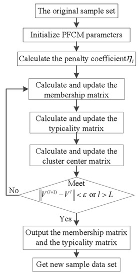
Figure 1.
The flow chart of the possibilistic fuzzy C-means (PFCM) algorithm.
2.2. Multi-Parameter Optimization of Support Vector Machine(SVM)
Support Vector Machine (SVM) is a new general machine learning method presented by Vapnik [37]. Traditional statistical research is in the case of sufficient samples or assuming an infinite number of samples, but in actual problems, there are few samples. According to the principle of structural risk minimization and the Vapnik-Chervonenkis(VC) dimension theory, SVM can combine the complexity of the model with the learning ability, find the optimal solution, and obtain better generalization ability. The classification theory of SVM is developed from the problem of linear separable binary classification. In the process of classification, the optimal classification hyperplane is constructed. The training samples are classified correctly according to the principle of least empirical risk, and the maximum classification interval is required to ensure the minimum confidence range. It has advantages in solving small-sized, nonlinear, high-dimensional problems [38,39,40]. The objective function of the SVM optimization problem is as follows:
where , ; is the Lagrange multiplier; C is the penalty factor; and is the kernel function which can transform a low-dimensional vector into a high-dimensional inner product.
The corresponding optimal classification function is as follows:
where is the optimal solution; .
In the above optimization problem, it is necessary to determine the kernel function . There are four kinds of kernel functions commonly used in SVM as follows: linear kernel function ; polynomial kernel function ; hyperbolic tangent kernels function ; and radial basis kernel function , where g is the kernel parameter.
Many studies show that radial basis kernel function is a better choice when there is not enough prior knowledge [41]. The radial basis kernel function is used as the kernel function in SVM. After that, the kernel function parameter g and the penalty factor C should be selected which are significant to establish the optimized SVM model.
The artificial bee colony (ABC) algorithm is an intelligent optimization algorithm inspired by biological behaviors proposed by Karaboga [42,43]. It mainly solves practical problems by simulating bees collecting honey. The ABC algorithm finds the global optimal solution through the local optimization behavior of bees. It is often used to solve multi-parameter optimization problems [44]. In the paper, the ABC algorithm is used to obtain the optimal penalty factor C and kernel parameter g. Compared with the genetic algorithm (GA), and particle swarm optimization algorithm (PSO), the ABC algorithm has the advantages of strong global optimization ability and few control parameters.
The multi-parameter optimization of SVM is as follows:
Step 1 Initialize the parameters in the ABC algorithm and SVM, i.e., the number of bee colonies, the number of honey sources, the maximum search number of honey sources (Limit), the current search number of honey sources, the maximum number of iterations (MaxIter), the search range of penalty factors C, and the search range of kernel function parameter g.
Step 2 Select the fitness function in the ABC algorithm. The purpose of optimizing the SVM parameters is to improve the accuracy of fault classification. The solution of the optimization problem can be regarded as a process for the bee to find the honey source. The fitness function is as follows:
where, is the fitness value of the i-th parameter, and is the objective function value of the i-th honey source.
Step 3 Employed bees search for the neighborhood of the current honey source according to Formula (12) and calculate the fitness of the new honey source according to Formula (11). If the fitness value of the new honey source is better than that of the original honey source, the new honey source position replaces the original honey source position, otherwise the original honey source remains unchanged.
where, is the value of the d-th dimension in the i-th new honey source; is the value of the d-th dimension in the i-th original honey source; R is a random number in [–1, 1]; and k is any honey source except the i-th honey source.
Step 4 After the employed bees complete the global search, onlooker bees select the honey source according to Formula (13), and then search for the neighborhood to get the new honey source according to Formula (12). If the fitness value of the new honey source is better than that of the original honey source, the new honey source position replaces the original honey source position, otherwise the original honey source remains unchanged.
where, is the probability that the i-th honey source is selected, is the fitness value of the i-th honey source, and N is the total number of honey sources.
Step 5 Judge whether the current search number of honey sources is bigger than the maximum search number of honey sources. If it is bigger, generate a new honey source according to Formula (14).
where, is the value of the j-th dimension of the i-th honey source, .
Step 6 Record the current optimal honey source and judge whether the termination condition is met. If the termination condition is met, skip to Step 7, otherwise skip to Step 3.
Step 7 Get the global optimal honey sources, which are the penalty factor C and kernel parameter g, to establish the optimized SVM model.
3. Fault Simulation of the PEM Fuel Cell System
The PEM fuel cell system can directly convert chemical energy into electricity through electrochemical reaction and produce water and heat at the same time. The PEM fuel cell simulator model uses controller strategies and nonlinear models presented by Pukrushpan et al. [1]. It is assumed that the system is in a constant temperature state, ignoring the influence of the double charge layer, and it is regarded as a rapid dynamic behavior near the electrode/electrolyte. Parameters commonly used in the PEM fuel cell simulator model are described in Table 1.

Table 1.
Parameters commonly used in the polymer electrolyte membrane (PEM) fuel cell simulator model.
The PEM fuel cell simulator model was established by Pukrushpan, J.T. in [1] and some parameters of the PEM fuel cell simulator model are from [45,46,47] based on actual product parameters. The PEM fuel cell simulator model is widely used for the fault diagnosis of the PEM fuel cell system [7,8,12,14], and represents the75kW fuel cell system with 381 cells. The PEM fuel cell simulator model includes the fuel cell stack model, the compressor model, the supply manifold model, the return manifold model, the air cooler model, and the humidifier model. The PEM fuel cell system block diagram is shown in Figure 2. The five faults are partially quoted from the literature [1,14] and the amplitude of characteristic parameters is reduced to ±10%. The faults in the PEM fuel cell simulator model are described in Table 2.
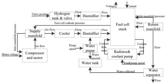
Figure 2.
The PEM fuel cell system block diagram [1].
Table 2.
Faults in the PEM fuel cell simulator model.
The characteristic parameters remain unchanged and Fault0 is in normal state. Equations (15)–(21) [1] are used to simulate Fault1–Fault4. According to the thermodynamic formula, the compressor torque is expressed as:
where, is the torque needed to drive the compressor, is the specific heat capacity of air, is the compressor speed, is the compressor efficiency, is the supply manifold pressure, is the pressure of the air, is the temperature of the air, is the ratio of the specific heats of the air, and is the air mass flow of compressor.
A lumped rotational parameter model with inertia is used to represent the compressor speed:
where is the combined inertia of the compressor and the motor, and is the compressor motor torque input.
The Fault1 state is simulated with the increment in the compressor constant . The Fault2 state is simulated with the increment in the compressor motor resistance :
where, is the motor mechanical efficiency, is the motor torque constant, is the compressor motor resistance, is the increment in the compressor motor resistance, is the motor electric constant, and is the increment in the motor electric constant.
The maximum mass of the vapor that the gas can hold is calculated from the vapor saturation pressure:
where, is the maximum mass of the vapor, is the saturation pressure of the vapor, is the gas constant of the vapor, and is the temperature of the stack. If , so , ; if ,so ,.
The total cathode pressure is the sum of oxygen, nitrogen, and vapor partial pressure:
where is the cathode pressure; is the cathode volume; , and are the partial pressure of oxygen, nitrogen, and vapor; , and are the gas constants of oxygen, nitrogen, and vapor.
Fault3 is simulated with the increment in the cathode outlet orifice constant :
where, is the increment in the cathode outlet orifice constant, is the cathode outlet orifice constant, is the air flow in the cathode outlet, is the cathode pressure, and is the return manifold pressure.
Fault 4 is simulated with the increment in the supply manifold outlet orifice constant :
where, is the outlet mass flow, is the increment in the supply manifold outlet orifice constant, and is the supply manifold outlet orifice constant.
4. Fault Diagnosis of the PEM Fuel Cell System
In this work, the Gaussian noise with variance of 0.1, 0.2, 0.5, and 1.0 are added to the PEM fuel cell simulator model, respectively. It is difficult to distinguish the Fault 0 to Fault 4 states in Table 2. Signals in a fault state are coupled with signals in other faults. Therefore, the traditional methods cannot diagnose the fault of the PEM fuel cell system effectively.
The Fault 0–4 states are simulated using the PEM fuel cell simulator model in the dynamic condition. Eight diagnostic variables are selected from the PEM fuel cell simulator model, and the eight diagnostic variables are fuel cell current(), fuel cell voltage(), compressor speed(), compressor outlet pressure(), compressor motor voltage(), compressor motor current(), hydrogen inlet pressure(), and air inlet pressure(). Taking the Fault4 state as an example, Gaussian noise with variance of 1.0 is added to the PEM fuel cell simulator model. The fuel cell current, fuel cell voltage, compressor speed, compressor outlet pressure, compressor motor voltage, compressor motor current, hydrogen inlet pressure, and air inlet pressure change with time, respectively, are shown in Figure 3, Figure 4, Figure 5, Figure 6, Figure 7, Figure 8, Figure 9 and Figure 10.
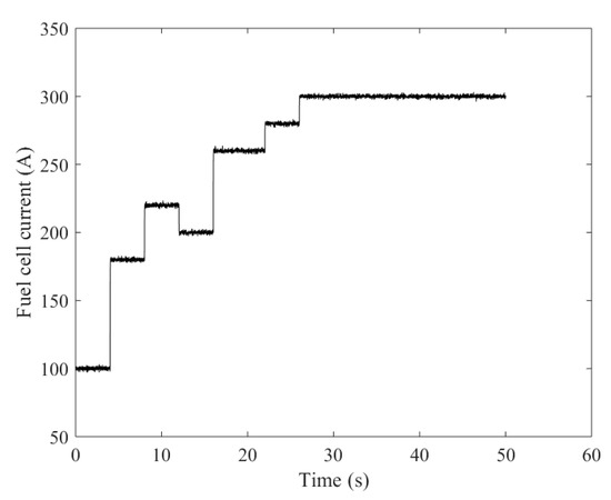
Figure 3.
Fuel cell current changes with time.
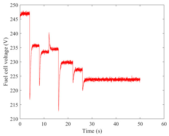
Figure 4.
Fuel cell voltage changes with time.
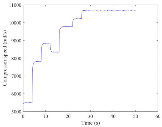
Figure 5.
Compressor speed changes with time.
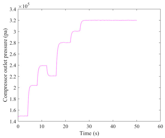
Figure 6.
Compressor outlet pressure changes with time.
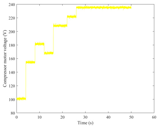
Figure 7.
Compressor motor voltage changes with time.
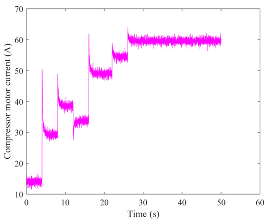
Figure 8.
Compressor motor current changes with time.

Figure 9.
Hydrogen inlet pressure changes with time.
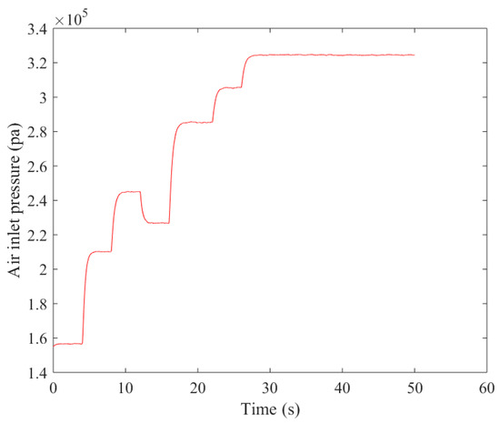
Figure 10.
Air inlet pressure changes with time.
In this paper, the Gaussian noise with variance of 0.1, 0.2, 0.5, and 1.0 are added to the PEM fuel cell simulator model, respectively. The PFCM algorithm is used to filter samples with membership and typicality less than 90% and optimize the original dataset. The filtered data is used as the sample dataset. The sample dataset are divided into two groups, one is the training set sample and the other is the testing set sample. The training set sample number is 670, and the testing set sample number is 335. The penalty parameter C and kernel function parameter g of SVM are optimized using the ABC algorithm, and then establish the optimized SVM model. The testing set sample is used to test the accuracy of the fault diagnosis method.
The fault diagnosis steps of the fuel cell system based on the PFCM-ABC-SVM method are as follows:
Step 1 Initialize the parameters in the PFCM-ABC-SVM method as follows: set the fuzzy parameters, m = 2, p = 2; set the terminating threshold = 10−6; set the maximum number of iterations L = 100; set the number of initial iterations l = 0; initialize the cluster center , initialize the membership matrix , and initialize the typicality matrix ; set the number of bee colonies n = 20; set the maximum search number of honey sources Limit = 100; set the current search number of honey sources d = 0; set the maximum number of iterations maxIter = 10; set the search range of penalty factor C: [0.01, 100]; and set the search range of kernel function parameter g: [0.01, 100].
Step 2 Get the original data of the PEM fuel cell system and select eight diagnostic variables. The eight diagnostic variables are fuel cell current, fuel cell voltage, compressor speed, compressor outlet pressure, compressor motor voltage, compressor motor current, hydrogen inlet pressure, and air inlet pressure.
Step 3 Establish the original dataset with eight diagnostic variables and normalize the original dataset using mapminmax Function in Matlab(R2018b).
Step 4 Adapt the PFCM algorithm to eliminate samples with membership and typicality less than 90%, filter the original dataset, and establish the sample dataset.
Step 5 Divide the sample dataset into the training set sample and the testing set sample.
Step 6 Optimize the penalty parameter C and kernel function parameter g of SVM using the ABC algorithm and establish the optimized SVM model.
Step 7 Diagnose faults by the optimized SVM model and obtain the diagnostic result. The fault diagnosis flow chart of the fuel cell system based on PFCM-ABC-SVM method is shown in Figure 11.
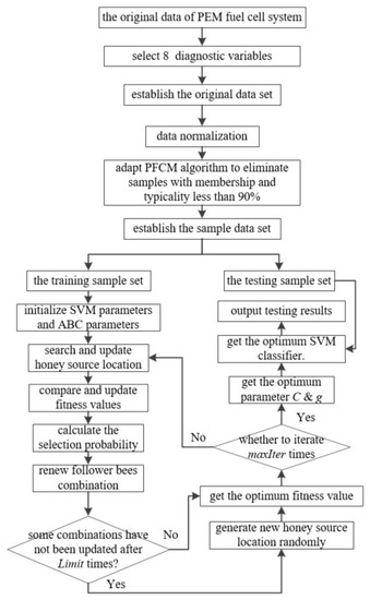
Figure 11.
Fault diagnosis flow chart of the fuel cell system based on the PFCM-ABC-SVM method.
When the Gaussian noise variance is 1.0, the PFCM-ABC-SVM method is compared with the GA-SVM, PSO-SVM and ABC-SVM methods. The comparison between the PFCM-ABC-SVM method and the other methods is shown in Table 3. The classification results of the PEMFC-ABC-SVM method when the Gaussian noise variance is 1.0 are shown in Figure 12. For the Fault 0–4 states, the accuracy of the training set sample is 95.67%, and the accuracy of the testing set sample is 92.84% using the PSO-SVM method; the accuracy of the training set sample is 95.82%, and the accuracy of the testing set sample is 94.03% using the ABC-SVM method; the accuracy of the training set sample is 97.46%, and the accuracy of the testing set sample is 97.31% using the PFCM-ABC-SVM method. Therefore, the PFCM-ABC-SVM method can effectively improve the accuracy of fault diagnosis of the PEM fuel cell system. The category label in Figure 12, “0” represents Fault0, “1” represents Fault1, “2” represents Fault2, “3” represents Fault3, and “4” represents Fault4. There are 335 samples in the testing set samples.
Table 3.
The comparison between the PFCM-ABC-SVM method and the other methods.
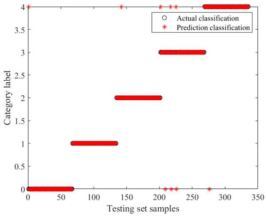
Figure 12.
The classification results of the PFCM-ABC-SVM method when the Gaussian noise variance is 1.0.
When the Gaussian noise variance is 0.5, the PFCM-ABC-SVM method is compared with the GA-SVM, PSO-SVM and ABC-SVM methods. The comparison between the PFCM-ABC-SVM method and the other methods is shown in Table 4. The classification results of the PEMFC-ABC-SVM method when the Gaussian noise variance is 0.5 are shown in Figure 13. The accuracy of the training set sample is 98.81% and the accuracy of the testing set sample is 97.91% using the PFCM-ABC-SVM method.
Table 4.
The comparison between the PFCM-ABC-SVM method and the other methods.
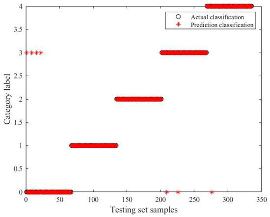
Figure 13.
The classification results of the PFCM-ABC-SVM method when the Gaussian noise variance is 0.5.
When the Gaussian noise variance is 0.2, the PFCM-ABC-SVM method is compared with the GA-SVM, PSO-SVM and ABC-SVM methods. The comparison between the PFCM-ABC-SVM method and the other methods is shown in Table 5. The classification results of the PEMFC-ABC-SVM method when the Gaussian noise variance is 0.2 are shown in Figure 14. The accuracy of the training set sample is 98.81%, and the accuracy of the testing set sample is 98.21% using the PFCM-ABC-SVM method.
Table 5.
The comparison between the PFCM-ABC-SVM method and the other methods.
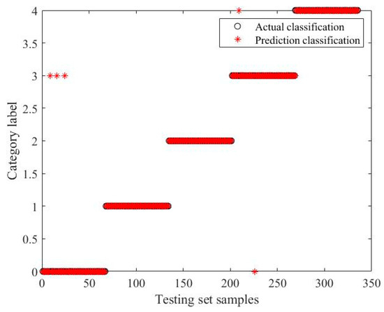
Figure 14.
The classification results of the PFCM-ABC-SVM method when the Gaussian noise variance is 0.2.
When the Gaussian noise variance is 0.1, the PFCM-ABC-SVM method is compared with the GA-SVM, PSO-SVM and ABC-SVM methods. The comparison between the PFCM-ABC-SVM method and the other methods is shown in Table 6. The classification results of the PEMFC-ABC-SVM method when the Gaussian noise variance is 0.1 are shown in Figure 15. The accuracy of the training set sample is 98.66%, and the accuracy of the testing set sample is 98.51% using the PFCM-ABC-SVM method.
Table 6.
The comparison between the PFCM-ABC-SVM method and the other methods.
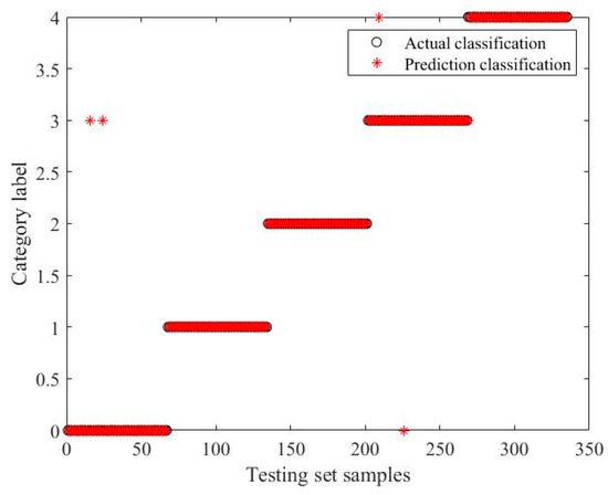
Figure 15.
The classification results of the PFCM-ABC-SVM method when the Gaussian noise variance is 0.1.
In order to illustrate the advantages of the PFCM-ABC-SVM method, the GA-SVM, PSO-SVM and ABC-SVM methods are compared with it, in this work. The results of fault diagnosis are shown in Table 3, Table 4, Table 5 and Table 6. Under the dynamic conditions with the variance of the Gaussian noise decreasing from 1.0 to 0.1, the accuracy of the testing set sample is as high as 98.51%. Comparing with the other methods, the PFCM-ABC-SVM method has a better effect in fault diagnosis of the PEM fuel cell system.
5. Conclusions
In this work, the PFCM-ABC-SVM method is proposed and verified by the PEM fuel cell simulator model. The Gaussian noise with variance of 0.1, 0.2, 0.5, and 1.0 are added to the PEM fuel cell simulator model, respectively, for fault diagnosis. The PFCM algorithm is used to filter samples with membership and typicality less than 90% and optimize the original dataset. The ABC algorithm is used to optimize the penalty factor C and kernel function parameter g, and the optimized SVM model is used to diagnose the faults of the PEM fuel cell system. The results show that under the dynamic conditions with the variance of the Gaussian noise decreasing from 1 to 0.1, the accuracy of the training set sample increases from 97.46% to 98.81%, and the accuracy of the testing set sample increases from 97.31% to 98.51%. The PFCM-ABC-SVM method is effective to diagnose the faults in the PEM fuel cell system, and it is better than other commonly used methods. The PFCM-ABC-SVM method has an advantage in solving the small-sized, nonlinear, and high-dimensional problems and furthermore, provides references for on-line fault diagnosis of a fuel cell system.
Author Contributions
Methodology, F.H.; writing—original draft preparation, F.H.; software, F.H. and Y.T.; data curation, Y.T.; writing—review and editing, Y.T. and Q.Z.; validation, Q.Z.; supervision, X.Z.; project administration, X.Z.; funding acquisition, X.Z. All authors have read and agreed to the published version of the manuscript.
Funding
This research was funded by the National Key Research and Development Program of China, grant number 2018YFB0105500.
Acknowledgments
The work was sponsored by the National Key Research and Development Program of China—Fuel Cell Bus Electric-Electric Deep Hybrid Power System Platform and Vehicle Development (no. 2018YFB0105500).
Conflicts of Interest
The authors declare no conflicts of interest.
Nomenclature
| PFCM | possibilistic fuzzy C-means clustering | ABC | artificial bee colony |
| SVM | support vector machine | PEM | polymer electrolyte membrane |
| LPV | linear parameter varying | TS | Takagi–Sugeno |
| FDI | fault detection and isolation | ANN | artificial neural network |
| EMD | empirical mode decomposition | EIS | electrochemical impedance spectroscopy |
| SVR | support vector regression | ANFIS | adaptive neuro-fuzzy inference systems |
| GS | grid search algorithm | GA | genetic algorithm |
| PSO | particle swarm optimization algorithm | FCM | fuzzy C-means clustering |
| PCM | possibilistic C-means clustering | C | penalty factor |
| g | kernel function parameter | terminating threshold | |
| L | maximum number of iterations | l | the number of initial iterations |
| penalty coefficient | Lagrange multiplier | ||
| Limit | maximum search number of honey sources | MaxIter | maximum number of iterations |
| compressor torque(N·m) | motor mechanical efficiency | ||
| the increment in the compressor motor resistance(Ω) | the increment in the motor electric constant(V/(rad/s)) | ||
| t | time(s) | the increment in the cathode outlet orifice constant(kg/(s·Pa)) | |
| air flow in the cathode outlet(g/s) | cathode pressure(pa) | ||
| return manifold pressure(pa) | outlet mass flow(g/s) | ||
| the increment in the supply manifold outlet orifice constant | supply manifold pressure(pa) | ||
| fuel cell current(A) | fuel cell voltage(V) | ||
| compressor speed(rad/s) | compressor outlet pressure(pa) | ||
| compressor motor voltage(V) | compressor motor current(A) | ||
| hydrogen inlet pressure(pa) | air inlet pressure(pa) |
References
- Pukrushpan, J.T.; Stefanopoulou, A.; Peng, H. Control of Fuel Cell Power Systems: Principles, Modeling, Analysis and Feedback Design; Springer: Berlin/Heidelberg, Germany, 2004. [Google Scholar]
- Benmouna, A.; Becherif, M.; Depernet, D.; Gustin, F. Fault diagnosis methods for proton exchange membrane fuel cell system. Int. J. Hydrog. Energy 2017, 42, 1534–1543. [Google Scholar] [CrossRef]
- Zheng, Z.; Petrone, R.; Pera, M.C.; Hissel, D. A review on non-model based diagnosis methodologies for PEM fuel cell stacks and systems. Int. J. Hydrog. Energy 2013, 38, 8914–8926. [Google Scholar] [CrossRef]
- Petrone, R.; Zheng, Z.; Hissel, D.; Pera, M.C. A review on model-based diagnosis methodologies for PEMFCs. Int. J. Hydrog. Energy 2013, 38, 7077–7091. [Google Scholar] [CrossRef]
- Isermann, R. Supervision, fault-detection and fault-diagnosis methods-an introduction. Control Eng. Pract. 1997, 5, 639–652. [Google Scholar] [CrossRef]
- Escobet, T.; Feroldi, D.; Lira, S.; Puig, V. Model-based fault diagnosis in PEM fuel cell systems. J. Power Sources 2009, 192, 216–223. [Google Scholar] [CrossRef]
- Feroldi, D. Fault Diagnosis and Fault Tolerant Control of PEM Fuel Cell Systems. In PEM Fuel Cells with Bio-Ethanol Processor Systems: A Multidisciplinary Study of Modelling, Simulation, Fault Diagnosis and Advanced Control; Springer: Berlin/Heidelberg, Germany, 2012; pp. 185–206. [Google Scholar]
- Rosich, A.; Sarrate, R.; Nejjari, F. On-line model-based fault detection and isolation for PEM fuel cell stack systems. Appl. Math. Model. 2014, 38, 2744–2757. [Google Scholar] [CrossRef]
- Lira, S.; Puig, V.; Quevedo, J.; Husar, A. LPV Model-Based Fault Diagnosis Using Relative Fault Sensitivity Signature Approach in a PEM Fuel Cell. In Proceedings of the 18th Mediterranean Conference on Control & Automation Congress Palace Hotel Marrakech, Marrakech, Morocco, 23–25 June 2010. [Google Scholar]
- Laghrouche, S.; Liu, J.; Ahmed, F.S.; Harmouche, M. Adaptive second-order sliding mode observer-based fault reconstruction for PEM fuel cell air-feed system. IEEE Trans. Control Syst. Technol. 2015, 23, 1098–1109. [Google Scholar] [CrossRef]
- Rotondo, D.; Fernandez, R.M.; Tornil, S.; Blesa, J. Robust fault diagnosis of proton exchange membrane fuel cells using a Takagi-Sugeno interval observer approach. Int. J. Hydrog. Energy 2016, 41, 2875–2886. [Google Scholar] [CrossRef]
- Kamal, M.M.; Yu, D.W.; Yu, D.L. Fault detection and isolation for PEM fuel cell stack with independent RBF model. Eng. Appl. Artif. Intell. 2014, 28, 52–63. [Google Scholar] [CrossRef]
- Steiner, N.Y.; Hissel, D.; Mocoteguy, P.; Candusso, D. Diagnosis of polymer electrolyte fuel cells failure modes (flooding & drying out) by neural networks modeling. Int. J. Hydrog. Energy 2011, 36, 3067–3075. [Google Scholar]
- Antoni, E.; Àngela, N.; Francisco, M. PEM fuel cell fault diagnosis via a hybrid methodology based on fuzzy and pattern recognition techniques. Eng. Appl. Artif. Intell. 2014, 36, 40–53. [Google Scholar]
- Shao, M.; Zhu, X.J.; Cao, H.F.; Shen, H.F. An artificial neural network ensemble method for fault diagnosis of proton exchange membrane fuel cell system. Energy 2014, 67, 268–275. [Google Scholar] [CrossRef]
- Damour, C.; Benne, M.; Brigitte, G.P.; Bessafi, M. Polymer electrolyte membrane fuel cell fault diagnosis based on empirical mode decomposition. J. Power Sources 2015, 299, 596–603. [Google Scholar] [CrossRef]
- Zheng, Z.; Pera, M.C.; Hissel, D.; Becherif, M. A double-fuzzy diagnostic methodology dedicated to online fault diagnosis of proton exchange membrane fuel cell stacks. J. Power Sources 2014, 271, 570–581. [Google Scholar] [CrossRef]
- Ibrahim, M.; Antoni, U.; Steiner, N.Y.; Jemei, S. Signal-based diagnostics by wavelet Transform for proton exchange membrane fuel cell. Energy Proced. 2015, 74, 1508–1516. [Google Scholar] [CrossRef]
- Pahon, E.; Steiner, N.Y.; Jemei, S.; Hissel, D. A signal-based method for fast PEMFC diagnosis. Appl. Energy 2016, 165, 748–758. [Google Scholar] [CrossRef]
- Mohammadi, A.; Djerdir, A.; Yousfi, S.N.; Khaburi, D. Advanced diagnosis based on temperature and current density distributions in a single PEMFC. Int. J. Hydrog. Energy 2015, 40, 15845–15855. [Google Scholar] [CrossRef]
- Silva, R.E.; Gouriveau, R.; Jeme, S.; Hissel, D. Proton exchange membrane fuel cell degradation prediction based on adaptive neuro-fuzzy inference systems. Int. J. Hydrog. Energy 2014, 39, 11128–11144. [Google Scholar] [CrossRef]
- Li, Q.; Chen, W.; Liu, Z.; Guo, A. Nonlinear multivariable modeling of locomotive proton exchange membrane fuel cell system. Int. J. Hydrog. Energy 2014, 39, 13777–13786. [Google Scholar] [CrossRef]
- Pei, P.; Li, Y.; Xu, H. A review on water fault diagnosis of PEMFC associated with the pressure drop. Appl. Energy 2016, 173, 366–385. [Google Scholar] [CrossRef]
- Zhao, X.W.; Xu, L.F.; Li, J.Q.; Fang, C. Faults diagnosis for PEM fuel cell system based on multi-sensor signals and principle component analysis method. Int. J. Hydrog. Energy 2017, 42, 18524–18531. [Google Scholar] [CrossRef]
- Huang, L.; Zeng, Q.; Zhang, R.M. Fuel Cell Engine Fault Diagnosis Expert System based on Decision Tree. In Proceedings of the IEEE 3rd Information Technology, Networking, Electronic and Automation Control Conference (ITNEC), Chengdu, China, 5–17 March 2019. [Google Scholar]
- Liu, J.Y.; Li, Q.; Chen, W.R.; Yan, Y. A Fast Fault Diagnosis Method of the PEMFC System Based on Extreme Learning Machine and Dempster-Shafer Evidence Theory. IEEE Trans. Transp. Electrif. 2019, 5, 271–284. [Google Scholar] [CrossRef]
- Bougatef, Z.; Abdelkrim, N.; Aitouche, A.; Abdelkrim, M.N. Fault detection of a PEMFC system based on delayed LPV observer. Int. J. Hydrog. Energy 2020, 45, 11233–11241. [Google Scholar] [CrossRef]
- Wang, X.D.; Liu, G.Y.; Xu, J.Y.; Jiang, J.M.; Huang, M.; Li, Q.F. Microstructure control and performance of electro-catalysis composite materials for oxygen evolution reaction (OER) in proton exchange membrane water electrolysis. Chin. Sci. Chem. 2014, 44, 1241–1254. [Google Scholar]
- Li, P.P.; Wang, M.; Chen, M.; Yang, Z.Y.; Wang, X.D. Influencing factors of electrochemical test of metal bipolar plate of PEMFC. Power Technol. 2018, 42, 1679–1681. [Google Scholar]
- Wilberforce, T.; Ijaodola, O.; Khatib, F.N.; Ogungbemi, E.O. Effect of humidification of reactive gases on the performance of a proton exchange membrane fuel cell. Sci. Total Environ. 2019, 688, 1016–1035. [Google Scholar] [CrossRef]
- Wilberforce, T.; El Hassan, Z.; Ogungbemi, E.; Ijaodola, O. A comprehensive study of the effect of bipolar plate (BP) geometry design on the performance of proton exchange membrane (PEM) fuel cells. Renew. Sustain. Energy Rev. 2019, 111, 236–260. [Google Scholar] [CrossRef]
- Wilberforce, T.; Khatib, F.N.; Ijaodola, O.S.; Ogungbemi, E. Numerical modelling and CFD simulation of a polymer electrolyte membrane (PEM) fuel cell flow channel using an open pore cellular foam material. Sci. Total Environ. 2019, 678, 728–740. [Google Scholar] [CrossRef]
- Wilberforce, T.; El Hassan, Z.; Khatib, F.N.; Al Makky, A. Development of Bi-polar plate design of PEM fuel cell using CFD techniques. Int. J. Hydrog. Energy 2017, 42, 25663–25685. [Google Scholar] [CrossRef]
- Chang, X.; Sun, J. Application of Fuzzy Clustering Based on Particle Swarm Optimization in Data Processing. Proc. CSU-EPSA 2015, 27, 78–83. [Google Scholar]
- Pal, N.R.; Pal, K.; Keller, J.M.; Bezdek, J.C. A Possibilistic Fuzzyc-Means Clustering Algorithm. IEEE Trans. Fuzzy Syst. 2005, 13, 517–530. [Google Scholar] [CrossRef]
- Pal, N.R.; Pal, K.; Keller, J.M. A New Hybrid C-means Clustering Model. In Proceeding of the IEEE International Conference on Fuzzy System, Budapest, Hungary, 25–29 July 2004; IEEE Press: Piscataway, NJ, USA, 2004; pp. 179–184. [Google Scholar]
- Vapnik, V.N. The Nature of Statistical Learning Theory, 2nd ed.; Springer: New York, NY, USA, 2000. [Google Scholar]
- Xiao, Y.; Wang, Y.J.; Ding, Z.T. The Application of Heterogeneous Information Fusion in Misalignment Fault Diagnosis of Wind Turbines. Energies 2018, 11, 1655. [Google Scholar] [CrossRef]
- Wu, D. Gear box fault diagnosis method based on support vector machine. J. Vib. Meas. Diagn. 2008, 28, 339–342. [Google Scholar]
- Azriel, R.; Wechser, H. Pattern recognition: Historical perspective and future directions. Int. J. Imaging Syst. Technol. 2000, 11, 101–116. [Google Scholar]
- Men, H.; Wu, Y.; Gao, Y. Application of Support Vector Machine to Pattern Classification. In Proceedings of the International Conference on Signal Processing, Beijing, China, 26–29 October 2008; IEEE: Piscataway, NJ, USA, 2008; pp. 1612–1615. [Google Scholar]
- Karaboga, D. An Idea Based on Honey Bee Swarm for Numerical Optimization; Technical Report-TR06; Erciyes University: Kayseri, Turkey, 2005. [Google Scholar]
- Karaboga, D.; Basturk, B. On the performance of artificial bee colony (ABC) algorithm. Appl. Soft Comput. 2008, 8, 687–697. [Google Scholar] [CrossRef]
- Karaboga, D.; Akay, B. A Comparative Study of Artificial Bee Colony Algorithm. Appl. Math. Comput. 2009, 214, 108–132. [Google Scholar] [CrossRef]
- Adams, J.; Yang, W.C.; Oglesby, K.; Osborne, K. The Development of Ford’s P2000 Fuel Cell Vehicle; SAE Paper: Detroit, MI, USA, 2000. [Google Scholar]
- Cunningham, J.; Hoffman, M.; Moore, R.; Friedman, D. Requirements for a flexible and realistic air supply model for incorporation into a fuel cell vehicle (FCV) system simulation. SAE Trans. 1999, 3191–3196. [Google Scholar]
- Nguyen, T.; White, R. A water and heat management model for proton-exchange-membrane fuel cells. J. Electrochem. Soc. 1993, 140, 2178–2186. [Google Scholar] [CrossRef]


© 2020 by the authors. Licensee MDPI, Basel, Switzerland. This article is an open access article distributed under the terms and conditions of the Creative Commons Attribution (CC BY) license (http://creativecommons.org/licenses/by/4.0/).