Article

The Schaake Shuffle Technique to Combine Solar and Wind Power Probabilistic Forecasting

by
Stefano Alessandrini
* and
Tyler McCandless
Research Applications Laboratory, National Center for Atmospheric Research (NCAR), Boulder, CO 80307-3000, USA
*
Author to whom correspondence should be addressed.
Energies 2020, 13(10), 2503; https://doi.org/10.3390/en13102503
Submission received: 24 January 2020 / Revised: 16 April 2020 / Accepted: 8 May 2020 / Published: 15 May 2020
(This article belongs to the Special Issue Applications of Artificial Intelligence in Renewable Energy)

Abstract

:
One way to mitigate the variability of wind and solar power generation is to install the corresponding plants in nearby locations. For example, in Kuwait, the facility at Shagaya Renewable Energy Park is located in a desert area with both photovoltaic panels and wind turbines that allow the continuous generation of renewable energy throughout the day. The National Center for Atmospheric Research (NCAR) has developed a system to generate probabilistic wind and solar predictions for the Shagaya facility. These predictions are based on the analog ensemble technique that post-processes the wind speed and solar irradiance predictions based on a combination of multiple models including the Weather Research and Forecasting (WRF) numerical model. The ensemble forecasts have 20 members and are generated independently at each wind and solar power production facility. Here we present a method based on the Schaake Shuffle (SS) technique to pair the ensemble members from the independent systems to obtain a unique ensemble prediction of the aggregated wind and solar generation. After reordering through the SS technique, the corresponding paired solar and wind power members can be summed to build a unique ensemble of combined generation that is statistically consistent, as verified by the presented metrics.

1. Introduction

One way to mitigate the variability of wind and solar power generation is to install these plants in an interconnected electric grid and to have them paired with energy storage systems. In fact, wind power production can compensate the lack of solar production during the night, allowing a continuous supply of renewable energy throughout a 24-h period. In recent years, given the growth of wind [1] and solar power [2] generation all over the world, there has been increasing interest in developing capabilities to manage grids or plants with solar and wind power installed together. One way to optimize the solar and wind plants hybrid production is through the resource assessment and planning stage. Depending on the geographic area, wind production can better complement solar production if, for example, the climatology indicates a daily cycle with stronger wind during the night hours. Several approaches to properly integrate solar and wind power resources were reviewed and proposed by the authors of [3,4]. In another study [5], the extent to which the combination of wind power and concentrated solar production could produce stable power in a particular region through proper siting was evaluated. Another component for optimal integration is quite often a forecasting system able to predict the aggregated production of solar and wind [6], which is highly variable in time due to the weather processes (solar radiation and wind speed) on which it depends. In fact, accurate and specific forecasting can help to mitigate strong fluctuations potentially induced in the electricity grid by facilitating the balancing [7,8]. For example, when dealing with aggregated wind and solar power generated from different geographic areas, accurate predictions can prevent an overload of a segment of the transmission grid in the case of concurrent production peaks [9]. For producers in countries that require predictions of their energy production, accurate forecasts can limit the penalties they have to pay; these penalties are commonly proportional to the forecast errors [10,11,12].
Wind and solar power predictions can be subdivided into two main groups: deterministic and probabilistic. A deterministic forecast provides a single power value for any future time, while a probabilistic forecast usually consists of multiple values. These values, commonly referred to as ensemble members, represent a Monte Carlo approximation of a probability density function (PDF) from which probabilities of future outcomes can be estimated. Probabilistic predictions not only provide a unique forecasted value for each time in the future (such as the mean or the median of the distribution) but they also provide additional information about the range of potential values. For example, by looking at the spread of the distribution (defined as the standard deviation about the ensemble members’ mean), one can be informed about the uncertainty of the forecast (being the spread proportional to the uncertainty). In addition, the probabilities of exceeding certain production levels can be estimated by counting the fraction of ensemble members greater than the threshold of interest. The value of probabilistic predictions in the renewable energy sector has been explored in several works, including trading in the day-ahead electricity markets [12]. It has been shown that trading future wind energy production using probabilistic wind power predictions can lead to higher economic benefits than those obtained by using deterministic forecasts alone [10]. The most complete reviews of the state of the art in wind power forecasting can be consulted in [13], while some recent deterministic and probabilistic wind power forecasting applications are addressed by the authors of [14,15,16,17]. Comprehensive reviews of the status of forecasting solar irradiance on different timescales for energy generation are reported in [18,19,20,21], while different forecasting techniques to predict solar power output are evaluated and compared in [16,22].
In the literature, two main approaches have been followed to generate probabilistic wind and solar power forecasting. In one approach, ensemble meteorological systems (e.g., a numerical weather prediction (NWP) ensemble) like the European Centre for Medium-Range Weather Forecasts (ECMWF) Ensemble Prediction System (EPS) [23,24] are used to obtain the set of the ensemble members of meteorological variables like wind speed and solar irradiance. The EPS is based on running a meteorological model multiple times, adding stochastic model perturbations to the initial conditions, or using different physic parameterizations. By integrating each of these runs in time and space, multiple realizations of the meteorological variables of interest (mainly solar irradiance and wind speed) are represented in the ensemble members. These meteorological values need to be converted to power values, a task which is typically accomplished by applying a power conversion curve specific for each turbine or farm. The other approach to generate probabilistic wind and solar forecasts consists of applying statistical post-processing techniques to the outputs of a single deterministic meteorological model. The most commonly used statistical techniques include the analog ensemble (AnEn) [25,26,27] and quantile regression (QR) [28]. Both techniques require a historical dataset of past forecasts and past concurrent observations.
In this paper, we focus on the AnEn method already applied for wind and solar power forecasting [9,15,29,30,31]. In the case of wind and solar power, the ensemble of forecasts is constituted by a set of historical observations. These observations are those concurrent to past NWP forecasts at the same lead time, chosen across the past runs most similar to the current forecast. There are some advantages of using the AnEn rather than a dynamical meteorological ensemble for power forecasts. First, the AnEn is based on just one deterministic run and therefore requires less computational time than a dynamical ensemble made of multiple runs of an NWP model. Second, there is no need to generate power conversion curves since the historical observations that are selected as the analogs to the forecast are already power values. For the 0–72-h forecast lead time in particular, the AnEn has been shown to be naturally calibrated and therefore provides a reliable quantification of the uncertainty [15,29]. In the case of NWP ensembles, there is often an under-dispersive behavior affecting the ensemble in the first three days, which means that the ensemble spread underestimates the forecast error [24,32]. For this reason, post-processing calibration techniques are often adopted to adjust the ensemble spread.
Considering the aforementioned benefits, the National Center for Atmospheric Research (NCAR), supported by the Kuwait Institute for Scientific Research (KISR), has developed a system based on the AnEn to generate wind and solar probabilistic predictions for the Shagaya Renewable Energy Park located in a desert area in western Kuwait, which is a combined wind and solar plant (see Section 2 for more details about Shagaya). For this application, the AnEn is based mainly on wind speed and solar irradiance deterministic predictions from the Dynamic Integrated Forecast System (DICast®) [7]. The ensemble power forecasts contain 20 members and are generated independently for each of the five wind turbines and of the two solar power plants.
A standard approach used to properly couple the ensemble members from forecast issued at different locations or from different meteorological variables at the same place is ensemble copula coupling (ECC), introduced in [33]. ECC is commonly applied after a raw ensemble consisting of multiple NWP runs with different initializations, and is calibrated through post-processing techniques applied independently for each univariate output variable. A sample is drawn from each post-processing predictive distribution, and the sampled values are then rearranged based on the rank order structure of the raw ensemble. ECC has been demonstrated to be effective for meteorological variables and can be applied to wind and solar power ensembles if these are obtained through the post-processing of an NWP ensemble (for example, [32]). In the case of AnEn or QR, in which the ensemble is derived from a single deterministic forecast, the ECC cannot be applied because the raw ensemble, used to provide the rank order structure, is not available.
We hereby present a novel method, as an alternative to ECC, to pair the ensemble members from each production unit to obtain a unique ensemble prediction of the aggregated wind and solar generation. The ensemble members provided by AnEn were statistically indistinguishable and were generated without a space–time correlation. We applied the Schaake Shuffle (SS) technique [34], widely used for hydrological applications, to reorder the ensemble members and recover the space–time variability of solar and wind power forecast time-series. With this technique, the ensemble members for a given forecast lead time were ranked and matched with the rank of solar or wind power past observations at the same hours appropriately selected across the historical record. The members were then reordered to match the original order of the selected historical data. Thus, the rank order structure of the post-processed members was provided by historical observations and not, like in ECC, by the raw members from an NWP ensemble. Using the SS, we aimed to recover the observed inter-plant power correlation and the observed temporal power autocorrelation. After the reordering through the SS, we could sum the corresponding paired solar and wind power members to build a unique ensemble of combined total generation. This unique ensemble is expected to preserve the attributes of the individual solar and wind power ensembles such as calibration and reliability.
This paper is organized as follows. In Section 2, a description of the Shagaya facility is provided. In Section 3, the power forecasting system and the SS technique are described. In Section 4, the performance of the forecasts is evaluated, while the conclusions are drawn in Section 5.

2. Shagaya Renewable Energy Park

We used data from the Shagaya Renewable Energy Park [35], which is located in western Kuwait at an elevation of approximately 240 meters at 29.20° N by 47.05° E, about 100 km west of Kuwait City. Phase 1 of the Shagaya Renewable Energy Park has 10 MW of photovoltaic (PV) solar power, split evenly between thin film and polysilicon panel technologies [36], and has 10 MW of wind power from five 2-MW wind turbines with a hub height of 78 m [37]. The climate around Shagaya is characterized as a hot, arid desert climate. The majority of the days in Kuwait are mostly sunny, with clouds and dust storms that happen infrequently, and a short season of occasional thunderstorms typically in or around November. The Shamal season (June, July, August) causes predominantly strong winds from the northwest over the Kuwait region due to the impacts of the Asian monsoon and the differential heating between the mountains to the north and the desert in the region around Shagaya. Outside of these months, the Shamal pattern rarely produces strong wind speeds during the day so the diurnal cycle and low-level jet formation are the predominant causes of significant wind speed changes. Figure 1 shows the average global horizontal irradiance (GHI) by hour of day and by season, which shows there are generally clear sky patterns in each of the seasons. The hub-height wind speeds at the Shagaya plant experience both seasonal and diurnal patterns, as shown in Figure 1, where it is evident that during the months of June through August, the Shamal pattern typically produces strong wind speeds during the entire day. Summer capacity factors for the 10-MW wind farm average between 60–70% during those three months. In the non-Shamal months, the diurnal pattern is more evident, with lower wind speeds during the day and stronger wind speeds at night due to the formation of a nocturnal low-level jet. The solar irradiance and solar power data used in this paper were recorded in five-minute intervals, while the wind speed and wind power data were recorded in ten-minute intervals. Both were then averaged to 15-min intervals to match the forecast intervals from the DICast model.

3. The Probabilistic Solar and Wind Power Forecasting System at Shagaya

In this section, the components of the forecasting system at Shagaya are described. These components include DICast®, the AnEn, and the SS algorithm. DICast is used to build the archive of deterministic forecasts of the meteorological variables of interest, which are mainly surface temperature, cloud cover, wind speed at hub height, and global horizontal irradiance (GHI). The AnEn takes the current meteorological DICast forecast as input and generates the wind and solar power ensemble predictions. The SS algorithm reorders the members to reestablish consistency across consecutive lead times and among production units (Figure 2).

3.1. The Dynamic Integrated Forecast System (DICast)

DICast® is an observation and model-based forecasting system that integrates NWP model forecasts and observations to produce site-specific tuned forecasts based on each model’s recent performance. DICast has been shown to improve upon the best members by around 10% for 10-m wind speed for the Conterminous United States [7]. In the DICast system implemented for the KISR, the integrated NWP models are as follows: the Weather Research and Forecasting model enhanced for solar irradiance prediction (WRF-Solar) [38,39], the U.S. Global Forecasting System (GFS), and Canada’s Global Environmental Multiscale (GEM) model. The system produces site-specific hourly forecasts of cloud cover, temperature, wind speed, wind power, global horizontal irradiance (GHI), and solar power. The first four hours have forward error correction applied, where the 4-h-ahead forecast is interpolated with the most recent observation as a blend of persistence and NWP modeling. In this study, we focused on the first 72 1-h time steps (i.e., the next three days at 1-h intervals) with the model initialization time at 00:00 UTC. DICast made predictions at each turbine and PV farm separately.

3.2. The Analog Ensemble Technique (AnEn)

The AnEn technique has been widely used for many applications, including renewable energy applications, and is described in several works. Here we provide a brief description and we recommend other works [15,26,29] for more details. In this work, the AnEn was applied after the DICast post-processing of the meteorological variables which is similar to what was carried out in [31], where a neural network was used as a model output statistic (MOS) to improve the raw NWP deterministic output. For each lead time (t) and target forecast in the testing dataset, the AnEn set of power forecasts was constituted by N power observations in the training dataset, where N was the number of ensemble members. The observations were those concurrent with the forecast at the same lead time, chosen across the training dataset based on their similarity to the target forecast. A Euclidean distance between the target and forecasts in the training dataset was used as a similarity criterion. It is worth mentioning that the AnEn does not use a function (power conversion curve) to convert the meteorological quantities into power. In fact, the analog forecasts are selected using only meteorological predictors, while the corresponding observed power values provide directly with the ensemble power predictions.
The dataset used to test our forecasting system was obtained from an archive from 1 September 2017 through to 1 December 2019 of 0–72-h DICast forecasts of 1-h average GHI, hub-height wind speed (WS) and direction (WD), 2-m temperature (2-m T), and cloud cover (CC), along with power observed at each turbine and PV farm. Only forecasts initialized at 00:00 UTC were considered. Data from 1 September 2017 to 30 November 2018 were used for training, while data from 1 December 2018 to 1 December 2019 were used for testing.
After some tuning over the training dataset, we set the number of members equal to 20. Regarding the optimal training dataset’s length for solar predictions, we found it beneficial to have at least the same meteorological season in the training that, in practice, means to have a historical archive longer than one year. As in [29,40,41], the meteorological predictors output from DICast were used for the computation of the distance and their weights were defined with a “brute force” approach, i.e., trying all the possible combinations. The combination leading to the lowest continuous ranked probability score (CRPS, see Appendix A) computed over the training dataset was chosen and kept fixed across the testing dataset. The weight optimization was carried out independently at each wind turbine and solar farm and the resulting weights are reported in Table 1. It is worth noting that wind speed (WS) and GHI received the highest weight when predicting wind power and solar power, respectively. The wind direction (WD) weight was small since Shagaya is located in a flat and homogeneous area where there is a low error dependency upon wind direction and the hub height wind speed has a strongly northwestern dominated pattern, especially in the summer season. The 2-m temperature (2-m T) received some weight in all the production units because of its influence on the efficiency of both solar panels and wind turbines. The weights were quite similar among the turbines and among solar farms given their proximity.

3.3. The Schaake Shuffle Technique (SS)

The AnEn algorithm is applied independently for every forecast lead time and at each solar farm and power turbine (hereafter referred to as production units, PUs). The order of the members is determined by the ranking of the Euclidean distance used as similarity criteria between the current forecast and the past analog forecasts. Hence, the first member in the ensemble is the past observation whose corresponding past forecast has the minimum distance, while the N-th member is the one with the maximum distance of the ranked selected members. As demonstrated in the next section, when this order is used to match the members across the PU and at subsequent lead times, the resulting inter-PU correlation structure from the ensemble members might not be the same as that of the observations. In addition, the forecast time-series from the single members may not preserve the autocorrelation structure of the observations.
To overcome this limitation, the SS method [34] is applied to reorder the AnEn members as in our previous work [41]. For each PU at a certain forecast lead time, the AnEn members are ranked accordingly with the rank of observed power at the same lead time from N dates randomly chosen from the training period, where N is the number of AnEn members. The selected dates must remain the same across the PU and forecast lead times to ensure inter-plant and temporal consistency. Several approaches are available for the selection of N dates. One is a random selection (RS) from the training dataset, which is what we used in this work. Other possibilities are the use of past N dates (PD) to the current forecast date or an analog (AD) approach as in [42]. We explored only the RS and PD options without noticing significant differences. As we were satisfied with the results using RS, we decided to not explore the AD approach.
Figure 3 illustrates the main steps of an example of the SS procedure with N = 5 and considering only one solar farm and one wind turbine for simplification. In Step (1), five dates are randomly chosen from the training period. In Step (2), for a specific PU and at lead time 0, five observed power values are selected from the five randomly chosen dates. In Step (3), the five observed power values are increasingly sorted and a function is established (fourth) linking the positions of these values before and after the sorting. In Steps (5) and (6), the five AnEn members for the target forecast in the testing period at the same lead time are increasingly ranked. In Step (7) the sorted members are reordered using the linking function previously established for the observations. In Step (8), the procedure is repeated for the subsequent lead times keeping the same dates. It should be noted that the new order of the ensemble members does not affect their skill for univariate probabilistic and deterministic metrics such as the continuous ranked probability score or the mean absolute error.

4. Verification

In this section, our goal is to assess whether the SS technique can improve the ability of individual AnEn members to match the observed temporal power autocorrelation. Also, we aim to verify whether the paired solar and wind power corresponding members can be summed to build a unique ensemble of combined total generation that preserves some attributes of the individual solar and wind power ensembles, such as calibration and reliability.

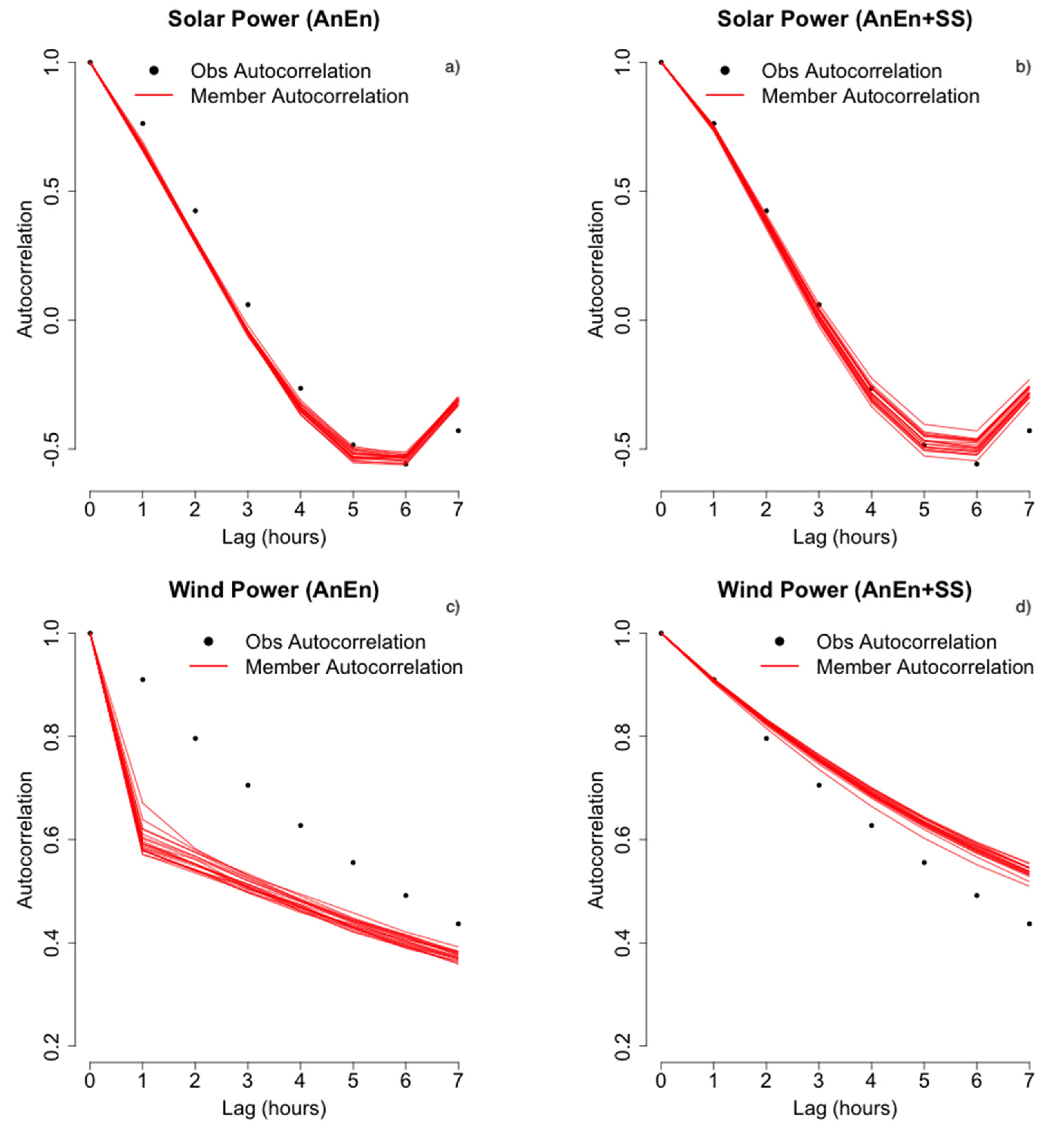
4.1. Temporal Auto Correlation of the Power Ensemble Members

In this subsection, we aim to verify if the forecast time series of the single members have similar temporal variability as the observations. In fact, one important characteristic of each ensemble member is to be able to represent a plausible realization of reality. This attribute is crucial, for example, when optimizing the charging cycles of an energy storage system (batteries or hydroelectric plants) connected to a renewable energy production facility or for maintenance planning. In fact, energy can be stored during production peaks or periods of low energy demands from the users and released at later times to make up for an incurred insufficient production or higher energy demand. In these cases, it is important to predict the number of consecutive hours in which the energy is going to stay below or above a given value.
In Figure 4, two examples of forecast time series are plotted for two randomly selected members at one solar farm and wind turbine. The forecast time series from the two members after the SS (right) are clearly smoother and more similar in terms of variability to the observations than before the SS (left). Therefore, the SS was able to reconstruct temporal consistency within each member that was able to represent a realistic time evolution similar to the observed one. A more quantitative assessment could be carried out by plotting the autocorrelation function (Figure 5) R for each member defined as
R ( τ ) = E [ F i ( t ) F i ( t + τ ) ]
where E is the mean operator, and F i ( t ) is the forecast of the ith at the lead time t, and τ is the time lag. The AnEn members (red lines) clearly underestimated the autocorrelation of the observations up to about 5 h for solar power and up to 6 h for wind power. When the SS technique was applied, the AnEn members exhibited very similar autocorrelation values to those of the observations in these time frames. The AnEn members’ forecast time series after the SS can have similar variability to the observations. For wind power, AnEn + SS slightly overestimated the observed autocorrelation. This tendency was inherited by the NWP model input to DICast, which tended to excessively enhance the wind speed daily cycle, resulting in an overestimate of the autocorrelation.

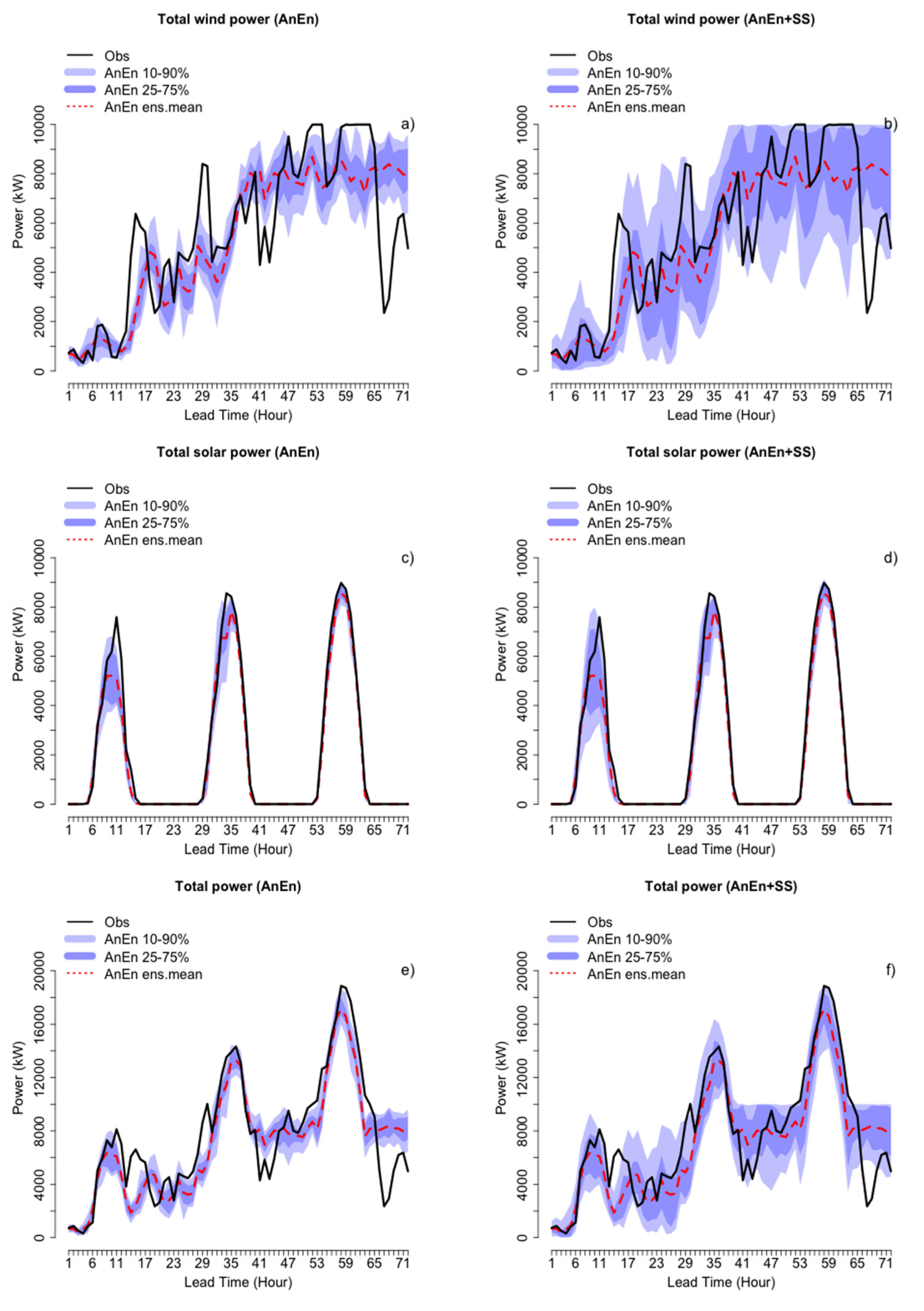
4.2. Ensemble of Total Generated Power

In this subsection, our goal is to analyze the performance in terms of some probabilistic metrics of the ensemble predictions of total power obtained by adding the individual members from the individual wind and solar PU. In Figure 6, an example of probabilistic forecast time series of the total wind power, the total solar power, and the total solar + wind power obtained by the AnEn and by the AnEn + SS is depicted. The 10th–90th and the 25th–75th percentile ranges were obtained from a 20-member ensemble where each member was the sum of the corresponding members of the individual PU. As expected, when applying the SS, the mean of the aggregated power did not change. In fact, the SS changed only the order of the values over which the mean was applied. The spread (defined as the standard deviation about the ensemble mean) from the AnEn + SS was clearly larger than that from the raw AnEn. In fact, without the SS, the members from different PU are not properly matched when adding them to build a unique ensemble. For example, if the quantiles below the median of the ensemble distribution from a PU are not properly matched with quantiles above the median from a different PU, the resulting ensemble distribution spread is reduced. A more quantitative analysis of the spread and other attributes of the ensembles of aggregated power is carried out in the next subsections.
An alternative approach to obtain the ensemble of total power (solar + wind) without the SS would apply the AnEn directly to total power. In this case, the AnEn should simultaneously use all the predictors defined in Table 1 to search for past analog forecasts, and the corresponding past observations of total power would build the ensemble. There are several disadvantages to this approach. Firstly, a separate forecast for solar and wind power would, of course, not be available. Secondly, the likelihood of finding good analog forecasts of total power is lower than that of finding analog forecasts independently for wind and solar. In fact, when searching for analogs for total power rather than for solar and wind separately, more meteorological predictors are needed, and more degrees of freedom are to be matched. As a consequence, given the same training length, the overall quality of the AnEn forecast is diminished. For example, assuming we apply the AnEn for predicting the total power, we should use simultaneously wind speed and GHI, which would probably receive about the same weight. On the other hand, we know that wind speed and GHI are almost irrelevant when trying to predict independently wind and solar power, respectively. It would be more difficult to find cases in our archive matching wind speed and GHI simultaneously. Lastly, it would not be possible to have single members providing a plausible time-series of the total power observations. In fact, as already mentioned in Section 4.1, the AnEn does not provide information about how to match the members at subsequent lead times.

4.2.1. Spread-Skill Consistency

In this section, our goal is to assess whether the ensemble predictions of aggregated solar and wind power of AnEn and AnEn + SS can quantify their own uncertainty by compiling the dispersion diagrams. In the dispersion diagrams, the overall average of the root mean squared error (RMSE) and spread are compared at any lead time [43]. A good correlation between RMSE and spread indicates that an ensemble system can predict its uncertainty [44] and ideally the ensemble spread should match the RMSE at any lead time. We direct the reader to Appendix B for the details on the proper RMSE and spread computation.
Dispersion diagrams can quantify the statistical consistency of ensemble predictions. Statistical consistency is achieved when the observations are indistinguishable from the ensemble members. In that case, the observations and the ensemble members can be seen as samples from the same distribution with the ensemble spread matching the RMSE of the ensemble mean. It is worth noting that the ensemble spread matching the RMSE is only a necessary condition for statistical consistency. In fact, if the ensemble and observed distributions are not Gaussian, their higher-order moments might not match, which would not be detected in a dispersion diagram. In Figure 7, the RMSE (solid) and the ensemble spread (dashed) are plotted as a function of the forecast lead time for the aggregated wind and solar power, and for the total (wind + solar) power. For all the three cases in the left panels (wind power, solar power, and total power), the spread (dashed line) underestimated the RMSE (solid lines) without using the SS. This means that by looking at the ensemble spread, one could receive a false sense of confidence regarding what to expect by the ensemble mean in terms of accuracy. In fact, the error (the absolute value of the difference between the ensemble mean and observation) is likely going to be larger than the ensemble spread. By using the SS algorithm, the RMSE/spread matching was improved in all three cases even though the ensembles were still slightly under-dispersive. It is worth noting that when the spread line intersected the bootstrap confidence intervals, the RMSE/spread difference is not statistically significant. There was a clear daily cycle of the error (RMSE) for wind, with a larger RMSE value at night. These more substantial errors can be attributed to the higher generation during the night due to the low-level jets. The overlapping of the solar error pattern, with a larger error around noon (lead times 10, 34, and 58), led to an additional daily peak in the RMSE of the total power.

4.2.2. Continuous Ranked Probability Score

The continuous ranked probability score (CRPS) [45] was thereafter used to assess the impact of applying the SS algorithm on the overall quality of the aggregated ensemble power predictions. In addition, the components of the CRPS were used to verify whether reliability or resolution was affected by the SS. We direct the reader to Appendix A for a more detailed discussion regarding the CRPS computation and its decomposition into the reliability (REL) and potential CRPS (CRPSPOT) that is obtained by subtracting the resolution (RES) from the uncertainty (UNC), i.e., CRPSPOT = UNC-RES.
In Figure 8, the CRPS is compiled for AnEn (black) and AnEn + SS (red) as a function of forecast lead time for the total wind and solar power, and the total (wind + solar) aggregated power. At the top of each panel, the values for the CRPS, CRPSPOT, and REL computed over all the lead times together are reported. AnEn + SS outperformed in all the cases the AnEn with a lower overall CRPS. On the left part of the panels, the CRPS values computed pooling all the lead times together are plotted together with the 5th–95th bootstrap confidence interval. Looking at the bootstrap intervals, the improvements of AnEn with respect to AnEn + SS were statistically significant only for the total wind power and the total wind + solar power. For the total solar power case, given the climatology of Shagaya with a high occurrence of predictable clear sky conditions, there were many forecast events with a small ensemble spread at the two solar farms. The effect of the SS reordering is, therefore, less important when the members are added to build the total solar power ensemble. Looking at the CRPS components, in all the cases AnEn + SS exhibited a lower (better) REL than AnEn, which determined the overall CRPS improvements. This improvement in reliability is consistent with the better RMSE/spread matching for AnEn + SS previously outlined. CRPSPOT was in general lower for AnEn than for AnEn + SS, indicating a better (higher value) resolution for AnEn. In fact, a better ability to discriminate the different observed frequencies from the climatological mean was achieved by the AnEn with a sharper ensemble (lower spread) than AnEn + SS. This improved resolution by the AnEn was gained at the cost of losing reliability, resulting in an overall degradation of the performance (higher CRPS).

5. Conclusions

A method to build a unique ensemble prediction of total power generated by different wind and solar production units (PUs) was explored. This method was based on the Schaake Shuffle (SS) algorithm in combination with the analog ensemble (AnEn) technique. The AnEn members, independently generated at each PU, were properly reordered and added together to obtain the ensemble members of the total power production. The proposed method (SS) can work with models like the AnEn or the quantile regression (QR) that generate the probabilistic forecast without using a numerical weather prediction (NWP) based ensemble. In fact, the SS makes use of past observations to define the rank order structure of the post-processed members. Thus, the SS is here proposed as an alternative to the ensemble copula coupling (ECC) that instead needs the raw members from an NWP ensemble for that purpose. An alternative approach to obtain the ensemble of total power (solar + wind) would apply the AnEn directly to total power. In this way, however, a separate forecast for solar and wind power would of course not be available. The likelihood of finding good analog forecasts of total power is lower than that of finding analog forecasts independently for wind and solar because more meteorological predictors are needed simultaneously in the former case.
We tested the AnEn + SS at the Shagaya Renewable Energy Park in Kuwait, where two solar farms and five wind turbines are installed with a 20-MW total capacity. It was demonstrated that the AnEn + SS allowed better statistical consistency and reliability than the raw AnEn when building the ensemble predictions of aggregated solar and wind power, and total solar + wind power. These attributes were verified by first looking at the root mean squared error (RMSE)/spread matching through the dispersion diagrams. As a matter of fact, the AnEn spread of total power underestimated the RMSE in all the cases, indicating an under-dispersive ensemble. In addition, the overall probabilistic performances of the ensembles of aggregated power were evaluated through the continuous ranking probability score (CRPS). In all the cases, AnEn + SS outperformed AnEn with a lower overall CRPS, even though the improvements were statistically significant only for wind power and total solar + wind power. These achievements could be attributed to a better reliability of AnEn + SS versus AnEn.
It was demonstrated that the SS could reconstruct similar temporal variability to the observed time series in the ensemble members, as verified by comparing their autocorrelation functions. This attribute is crucial, for example, when optimizing the charging cycles of an energy storage system (batteries or hydroelectric power plants) or for maintenance planning. In fact, in these cases, it is important to predict the number of consecutive hours in which the energy is going to stay below or above a given value.
It is worth noting that the SS technique could also be used with postprocessing techniques other than the AnEn like the ensemble model output statistic (EMOS) [30,46] or QR. With these techniques, like for the AnEn, the information on how to match the quantiles at different locations, PUs, or at consecutive lead times is not available. In addition, there is no significant computational cost added to the AnEn when running the SS.

Author Contributions

Conceptualization, S.A.; methodology, S.A. and T.M.; software, S.A.; validation, S.A. and T.M.; formal analysis, S.A.; investigation, S.A. and T.M.; writing—original draft preparation, S.A. and T.M; writing—review and editing, S.A. and T.M.; visualization, S.A. All authors have read and agreed to the published version of the manuscript.

Funding

This work has been funded by the Kuwait Institute for Scientific Research (KISR).

Acknowledgments

This material is based upon work supported by the National Center for Atmospheric Research, which is a major facility sponsored by the National Science Foundation under Cooperative Agreement No. 1852977. The authors wish to thank Simone Sperati and Luca Delle Monache for their contribution in the initial implementation of the Schaake shuffle algorithm.

Conflicts of Interest

The authors declare no conflict of interest.

Appendix A

The continuous ranked probability score (CRPS) is computed to assess the overall quality of a probabilistic prediction [47]. It can be expressed as:
C R P S = 1 N n = 1 N ( F i f ( x ) F i 0 ( x ) ) 2 d x
where F i f ( x ) is the cumulative distribution function (CDF) of the probabilistic forecast and F i 0 ( x ) is the CDF of the observation for the ith ensemble prediction/observation pair, and N is the number of available pairs. [45] showed that the CRPS reduces to mean absolute error (MAE) when considering a deterministic (single member) forecast, with a lower value of CRPS indicating better skill, and 0 being a perfect score. The CRPS has been computed by numerical integration techniques. We have used the function “crpsDecompostion” provided in the software library “verification” [48] to compute the CRPS through numerical integration techniques. As demonstrated in [45], the CRPS can be decomposed into three components similarly to the Brier score [49]: reliability (REL), resolution (RES), and uncertainty (UNC). Even though the CRPS can be conceptualized as the Brier score integrated over all the possible events, its components (REL, RES, and UNC) do not numerically match the integrated components of the Brier score.
The REL component measures the statistical consistency of the ensemble system (the lower, the better); that is, how well the forecasted probabilities match the observed frequencies. The REL attribute may also be assessed by compiling the rank histograms [50]. The RES component (the higher the better) measures how much better a system performs compared to a climatological forecast, where the climatological forecast is the single probability of an event as observed in the historical dataset. In general, the resolution attribute of a system reflects how well the different forecast frequency classes can separate the different observed frequencies from the climatological mean. The UNC component, which depends only on the observations, measures the variability of the observations reflecting the predictability associated with the available data set. More specifically, CRPS can be expressed as CRPS = REL + CRPSPOT, where CRPSPOT is the potential CRPS and can be expressed as CRPSPOT = UNC − RES. The CRPSPOT is the CRPS that could be obtained if a forecasting system would become perfectly reliable (REL = 0). For details about mathematical formulations of the three components, we direct the reader to [45].

Appendix B

As demonstrated by [43], an appropriate way to compute the RMSE for a comparison with the ensemble spread is to follow the equation:
R M S E ( t ) = 1 T i = 1 T N N + 1 [ f ¯ i ( t ) o ¯ i ( t ) ] 2
where T is the number of forecast events for the lead time t, N is the number of ensemble members.
The ensemble spread s should be derived from:
s ( t ) = 1 T i = 1 T j = 1 N 1 N 1 [ e i , j ( t ) e ¯ i ( t ) ] 2
where the overbar indicates the mean over the ensemble members j.

References

  1. WWEA Wind Power Istalled Capacity. Available online: https://wwindea.org/information-2/information/ (accessed on 28 August 2019).
  2. IEA Solar Installed Capacity. Available online: https://www.iea.org/topics/renewables/solar/ (accessed on 28 August 2019).
  3. Jurasz, J.; Canales, F.A.; Kies, A.; Guezgouz, M.; Beluco, A. A review on the complementarity of renewable energy sources: Concept, metrics, application and future research directions. Sol. Energy 2020, 195, 703–724. [Google Scholar] [CrossRef]
  4. Widén, J.; Carpman, N.; Castellucci, V.; Lingfors, D.; Olauson, J.; Remouit, F.; Bergkvist, M.; Grabbe, M.; Waters, R. Variability assessment and forecasting of renewables: A review for solar, wind, wave and tidal resources. Renew. Sustain. Energy Rev. 2015, 44, 356–375. [Google Scholar] [CrossRef]
  5. Santos-Alamillos, F.J.; Pozo-Vázquez, D.; Ruiz-Arias, J.A.; Von Bremen, L.; Tovar-Pescador, J. Combining wind farms with concentrating solar plants to provide stable renewable power. Renew. Energy 2015, 76, 539–550. [Google Scholar] [CrossRef]
  6. Kariniotakis, G.; Martí, I.; Casas, D.; Pinson, P.; Nielsen, T.S.; Madsen, H.; Giebel, G.; Usaola, J.; Sanchez, I. What performance can be expected by short-term wind power prediction models depending on site characteristics? In Proceedings of the EWC 2004 Conference, Taipei, Taiwan, 4–8 December 2004; pp. 22–25. [Google Scholar]
  7. Mahoney, W.P.; Parks, K.; Wiener, G.; Liu, Y.; Myers, W.L.; Sun, J.; Delle Monache, L.; Hopson, T.; Johnson, D.; Haupt, S.E. A wind power forecasting system to optimize grid integration. IEEE Trans. Sustain. Energy 2012, 3, 670–682. [Google Scholar] [CrossRef]
  8. Zugno, M.; Conejo, A.J. A robust optimization approach to energy and reserve dispatch in electricity markets. Eur. J. Oper. Res. 2015, 247, 659–671. [Google Scholar] [CrossRef] [Green Version]
  9. Davò, F.; Alessandrini, S.; Sperati, S.; Delle Monache, L.; Airoldi, D.; Vespucci, M.T. Post-processing techniques and principal component analysis for regional wind power and solar irradiance forecasting. Sol. Energy 2016, 134, 327–338. [Google Scholar] [CrossRef] [Green Version]
  10. Alessandrini, S.; Davò, F.; Sperati, S.; Benini, M.; Delle Monache, L. Comparison of the economic impact of different wind power forecast systems for producers. Adv. Sci. Res. 2014, 11, 49–53. [Google Scholar] [CrossRef] [Green Version]
  11. Roulston, M.S.; Kaplan, D.T.; Hardenberg, J.; Smith, L.A. Using medium-range weather forcasts to improve the value of wind energy production. Renew. Energy 2003, 28, 285–602. [Google Scholar] [CrossRef]
  12. Zugno, M.; Jõnsson, T.; Pinson, P. Trading wind energy on the basis of probabilistic forecasts both of wind generation and of market quantities. Wind Energy 2013, 16, 909–926. [Google Scholar] [CrossRef] [Green Version]
  13. Giebel, G.; Brownsword, R.; Kariniotakis, G.; Denhard, M.; Draxl, C. The State-of-ohe-Art in Short-Term Prediction of Wind Power a Literature Overview, 2nd ed.; ANEMOS.plus; Available online: https://doi.org/10.11581/DTU:00000017 (accessed on 28 August 2019).
  14. Pinson, P. Very-short-term probabilistic forecasting of wind power with generalized logit-normal distributions. J. R. Stat. Soc. Ser. C Appl. Stat. 2012, 61, 555–576. [Google Scholar] [CrossRef]
  15. Alessandrini, S.; Delle Monache, L.; Sperati, S.; Nissen, J.N. A novel application of an analog ensemble for short-term wind power forecasting. Renew. Energy 2015, 76, 768–781. [Google Scholar] [CrossRef]
  16. Sperati, S.; Alessandrini, S.; Pinson, P.; Kariniotakis, G. The “Weather intelligence for renewable energies” benchmarking exercise on short-term forecasting of wind and solar power generation. Energies 2015, 8, 9594–9619. [Google Scholar] [CrossRef] [Green Version]
  17. Cassola, F.; Burlando, M. Wind speed and wind energy forecast through Kalman filtering of Numerical Weather Prediction model output. Appl. Energy 2012, 99, 154–166. [Google Scholar] [CrossRef]
  18. Diagne, M.; David, M.; Lauret, P.; Boland, J.; Schmutz, N. Review of solar irradiance forecasting methods and a proposition for small-scale insular grids. Renew. Sustain. Energy Rev. 2013, 21, 65–76. [Google Scholar] [CrossRef] [Green Version]
  19. Heinemann, D.; Lorenz, E.; Girodo, M. Forecasting of solar radiation. In Solar Energy Resource Management for Electricity Generation from Local Level to Global Scale; Nova Science Publishers: New York, NY, USA, 2006; pp. 83–94. ISBN 1594549192. [Google Scholar]
  20. Yang, D.; Kleissl, J.; Gueymard, C.A.; Pedro, H.T.C.; Coimbra, C.F.M. History and trends in solar irradiance and PV power forecasting: A preliminary assessment and review using text mining. Sol. Energy 2018, 168, 60–101. [Google Scholar] [CrossRef]
  21. Inman, R.H.; Pedro, H.T.C.; Coimbra, C.F.M. Solar forecasting methods for renewable energy integration. Prog. Energy Combust. Sci. 2013, 39, 535–576. [Google Scholar] [CrossRef]
  22. Pedro, H.T.C.; Coimbra, C.F.M. Assessment of forecasting techniques for solar power production with no exogenous inputs. Sol. Energy 2012, 86, 2017–2028. [Google Scholar] [CrossRef]
  23. Molteni, F.; Buizza, R.; Palmer, T.N.; Petroliagis, T. The ECMWF ensemble prediction system: Methodology and validation. Q. J. R. Meteorol. Soc. 1996, 122, 73–119. [Google Scholar] [CrossRef]
  24. Alessandrini, S.; Sperati, S.; Pinson, P. A comparison between the ECMWF and COSMO Ensemble Prediction Systems applied to short-term wind power forecasting on real data. Appl. Energy 2013, 107, 271–280. [Google Scholar] [CrossRef]
  25. Hamill, T.M.; Whitaker, J.S. Probabilistic quantitative precipitation forecasts based on reforecast analogs: Theory and application. Mon. Weather Rev. 2006, 134, 3209–3229. [Google Scholar] [CrossRef]
  26. Monache, L.D.; Anthony Eckel, F.; Rife, D.L.; Nagarajan, B.; Searight, K. Probabilistic weather prediction with an analog ensemble. Mon. Weather Rev. 2013, 141, 3498–3516. [Google Scholar] [CrossRef] [Green Version]
  27. Alessandrini, S.; Sperati, S.; Delle Monache, L. Improving the analog ensemble wind speed forecasts for rare events. Mon. Weather Rev. 2019, 147, 2677–3692. [Google Scholar] [CrossRef]
  28. Bremnes, J.B. Probabilistic wind power forecasts using local quantile regression. Wind Energy 2004, 7, 47–54. [Google Scholar] [CrossRef]
  29. Alessandrini, S.; Delle Monache, L.; Sperati, S.; Cervone, G. An analog ensemble for short-term probabilistic solar power forecast. Appl. Energy 2015, 157, 95–110. [Google Scholar] [CrossRef] [Green Version]
  30. Junk, C.; Monache, L.D.; Alessandrini, S. Analog-based ensemble model output statistics. Mon. Weather Rev. 2015, 143, 2909–2917. [Google Scholar] [CrossRef]
  31. Cervone, G.; Clemente-Harding, L.; Alessandrini, S.; Delle Monache, L. Short-term photovoltaic power forecasting using Artificial Neural Networks and an Analog Ensemble. Renew. Energy 2017, 108, 274–286. [Google Scholar] [CrossRef] [Green Version]
  32. Sperati, S.; Alessandrini, S.; Delle Monache, L. An application of the ECMWF Ensemble Prediction System for short-term solar power forecasting. Sol. Energy 2016, 133, 437–450. [Google Scholar] [CrossRef] [Green Version]
  33. Schefzik, R.; Thorarinsdottir, T.L.; Gneiting, T. Uncertainty quantification in complex simulation models using ensemble copula coupling. Stat. Sci. 2013, 28, 616–640. [Google Scholar] [CrossRef]
  34. Clark, M.; Gangopadhyay, S.; Hay, L.; Rajagopalan, B.; Wilby, R. The Schaake shuffle: A method for reconstructing space-time variability in forecasted precipitation and temperature fields. J. Hydrometeorol. 2004, 5, 243–262. [Google Scholar] [CrossRef] [Green Version]
  35. KISR 2019 Kuwait Energy Outlook: Sustaining Prosperity Through Strategic Energy Management. Kuwait Institute for Scientific Research: Shuwaikh, Kuwait. Available online: https://www.arabstates.undp.org/content/dam/rbas/doc/EnergyandEnvironment/KEO_report_English.pdf (accessed on 8 October 2019).
  36. Al-Rasheedi, M.A.; Gueymard, C.A.; Al-Khayat, M.H.; Ismail, A.H.; Lee, J.A.; Al-Duaj, H. Performance evaluation of a utility-scale dual-technology photovoltaic power plant at the Shagaya Renewable Energy Park in Kuwait. Renew. Sustain. Energy Rev. 2020. Submitted. [Google Scholar]
  37. Naegele, S.M.; McCandless, T.C.; Greybush, S.J.; Young, G.S.; Haupt, S.E.; Al-Rasheedi, M. Climatology of wind variability for the Kuwait region. Renew. Sustain. Energy Rev. 2020. Accepted. [Google Scholar]
  38. Jiménez, P.A.; Alessandrini, S.; Haupt, S.E.; Deng, A.; Kosovic, B.; Lee, J.A.; Monache, L.D. The role of unresolved clouds on short-range global horizontal irradiance predictability. Mon. Weather Rev. 2016, 144, 3099–3107. [Google Scholar] [CrossRef]
  39. Jimenez, P.A.; Hacker, J.P.; Dudhia, J.; Haupt, S.E.; Ruiz-Arias, J.A.; Gueymard, C.A.; Thompson, G.; Eidhammer, T.; Deng, A. WRF-SOLAR: Description and clear-sky assessment of an augmented NWP model for solar power prediction. Bull. Am. Meteorol. Soc. 2016, 97, 1249–1264. [Google Scholar] [CrossRef]
  40. Junk, C.; Monache, L.D.; Alessandrini, S.; Cervone, G.; Von Bremen, L. Predictor-weighting strategies for probabilistic wind power forecasting with an analog ensemble. Meteorol. Z. 2015, 24, 361–379. [Google Scholar] [CrossRef]
  41. Sperati, S.; Alessandrini, S.; Delle Monache, L. Gridded probabilistic weather forecasts with an analog ensemble. Q. J. R. Meteorol. Soc. 2017, 143, 2874–2885. [Google Scholar] [CrossRef]
  42. Schefzik, R. A similarity-based implementation of the Schaake shuffle. Mon. Weather Rev. 2016, 144, 1909–1921. [Google Scholar] [CrossRef] [Green Version]
  43. Fortin, V.; Abaza, M.; Anctil, F.; Turcotte, R. Corrigendum to Why should ensemble spread match the RMSE of the ensemble mean? J. Hydrometeor. 2014, 15, 1708–1713. [Google Scholar] [CrossRef]
  44. Hopson, T.M. Assessing the ensemble spread-error relationship. Mon. Weather Rev. 2014, 142, 1125–1142. [Google Scholar] [CrossRef]
  45. Hersbach, H. Decomposition of the continuous ranked probability score for ensemble prediction systems. Weather Forecast. 2000, 15, 559–570. [Google Scholar] [CrossRef]
  46. Gneiting, T.; Raftery, A.E.; Westveld, A.H.; Goldman, T. Calibrated probabilistic forecasting using ensemble model output statistics and minimum CRPS estimation. Mon. Weather Rev. 2005, 133, 1098–1118. [Google Scholar] [CrossRef]
  47. Brown, T.A. Admissible Scoring Systems for Continuous Distributions; Rand Corp.: Santa Monica, CA, USA, 1974. [Google Scholar]
  48. NCAR-Research Applications Laboratory (2015). Verification: Weather Forecast Verification Utilities. R package version 1.42. Available online: https://CRAN.R-project.org/package=verification (accessed on 1 December 2019).
  49. Brier, G.W. Verification of forecasts expressed in terms of probability. Mon. Weather Rev. 1950, 78, 1–3. [Google Scholar] [CrossRef]
  50. Hamill, T.M. Interpretation of rank histograms for verifying ensemble forecasts. Mon. Weather Rev. 2001, 129, 550–560. [Google Scholar] [CrossRef]
Figure 1. Plot of the average hub-height wind speed by hour of the day (UTC) and by season from 21 Dec 2017 through to 20 Dec 2018 (a) and global horizontal irradiance (GHI) by hour of the day and by season (b).
Energies 13 02503 g001
Figure 2. Scheme of the probabilistic forecasting system built for the Shagaya plant. DICast: Dynamic Integrated Forecast System; AnEn: analog ensemble; SS: Schaake Shuffle.
Energies 13 02503 g002
Figure 3. Main steps of the Schaake shuffle algorithm. For sake of simplicity, only 5 ensemble members and 2 production units (1 solar farm and 1 wind turbine) are shown in this description.
Energies 13 02503 g003
Figure 4. Example of solar power and wind power predictions from 2 randomly selected analog ensemble (AnEn), (a,c) and AnEn + Schaake shuffle (SS), (b,d) ensemble members.
Energies 13 02503 g004
Figure 5. Observed (black) and predicted (ensemble members, red) autocorrelation of power with (b,d) and without Schaake shuffle (SS), (a,c) as a function of time lag for 1 PV farm (a,b) and 1 wind turbine (c,d).
Energies 13 02503 g005
Figure 6. Example of analog ensemble (AnEn), (a,c,e) and AnEn + Schaake shuffle (SS), (b,d,f) ensemble forecast for total wind power (a,b), total solar power (c,d) and total wind + solar power (e,f). The shaded area indicates the 10th–90th and the 25th–75th quantile range, and the solid black line the verifying observations.
Energies 13 02503 g006
Figure 7. Root mean squared error (solid) and spread (dashed) of the analog ensemble (AnEn), (a,c,e) and AnEn + Schaake shuffle (SS), (b,d,f) ensemble predictions of total wind power (a,b), total solar power (c,d), and total wind + solar power (e,f).
Energies 13 02503 g007
Figure 8. Continuous ranked probability score (CRPS) versus lead time for analog ensemble (AnEn), (black) and AnEn + Schaake shuffle (SS), (red) for total wind power (a), total solar power (b), and total solar + wind power (c). On the left part of the panels, the CRPS values computed pooling all the lead times together are plotted together with the 5th–95th bootstrap confidence interval. At the top of the panels, values of the CRPS, the potential CRPS (CRPSPOT), and the reliability (REL) are indicated.
Energies 13 02503 g008
Table 1. Weights of the meteorological predictors for each wind turbine and solar farm. The predictors indicated by NT were not tested. WS: wind speed; WD: wind direction; 2-M T: 2-m temperature; PV: photovoltaic.
Production UnitGHI2-MTWSWDCloud Cover
Turbine 1NT0.10.80.1NT
Turbine 2NT0.0.90.1NT
Turbine 3NT0.10.80.1NT
Turbine 4NT0.10.80.1NT
Turbine 5NT0.10.80.1NT
PV farm 10.50.1NTNT0.4
PV farm 20.50.2NTNT0.3

