Modeling of Interconnected Infrastructures with Unified Interface Design toward Smart Cities

Abstract

In recent years, there have been tendencies to enable smart cities with interconnected infrastructures and communities. Current engineering design and operation practices are limited to handling individual systems with modeling and simulation, as well as control systems. This paper presents a holistic approach with engineering practice to design and operate interconnected systems as part of smart cities. The approach is based on modeling individual physical systems and associated processes and identifying key performance indicators to evaluate each system and interconnected systems with an understanding of the coupling among systems to increase the overall performance of interconnected systems. The multi-objective optimization technique is proposed to achieve the best performance based on system design, control, and operation parameters. Due to the multidimensional nature of the interconnected systems, a unified interface system with modular design is proposed to achieve the highest overall performance of the interconnected systems with standardized interactions among state variables and performance measures. The proposed approach can allow dynamic updates of the interconnected systems based on model libraries of each system and process. A case study is presented of interconnected energy–water–transportation–waste facilities, whereby modeling is discussed, and performance measures are evaluated for different scenarios using the unified interface design.

1. Introduction

The United Nations 2030 agenda for sustainable development stated the need for reliable, quality, and timely data to provide evidence-based analysis as part of Sustainable Development Goals (SDGs) [1]. The analysis showed an increase in population by more than 1% yearly, which leads to more demand on energy and related resources. Energy is essential for water, transportation, food, health, and waste management facilities and infrastructures. The focus on energy grids has led to several initiatives for moving centralized power grids to decentralized grids while integrating renewable energy. The analysis of grid-connected and standalone structures revealed techno-economic and environmental assessments to evaluate energy infrastructures [2]. To optimize the design of energy infrastructures, a survey was conducted to identify the main engineering design parameters for reaching the optimum energy grids and associated components to meet load and demand profiles [3]. The analysis of detailed cost factors of power grids while considering the population and associated factors was optimized and applied to many regions and countries worldwide [4]. The progress made in energy infrastructures requires a proper study on energy management based on a simulation that can evaluate the planning scenarios and strategies to reduce performance measures such as GHG emissions [5]. Energy system analysis includes the impacts of district heating as part of energy flow analysis optimized with computational intelligence algorithms [6]. There are a number of proposed approaches that presented energy hubs for designing energy infrastructures with optimized algorithms to meet load demand from household appliances and charging electric vehicles (EVs) with vehicle-to-grid (V2G) options [7]. Different designs of energy hubs have been analyzed with examples from agriculture infrastructures [8]. The energy infrastructures can be carefully selected and designed in view of market operation with combined biofuel, heat, electricity, and associated technologies, such as combined heat and power (CHP) [9]. Smart energy systems and smart energy grids offer a number of useful approaches to enhance energy infrastructures with flexibility and optimization [10]. Power management can be introduced with hybrid energy systems, including renewable energy resources (RES) and energy storage in view of uncertainties of RES such as wind, while intelligent optimization algorithms are employed [11]. Smart energy systems are widely implemented in other city infrastructures such as agriculture and irrigation, where simulation models and experimental models have shown optimum performance for integrated energy, water, and farm parameters such as soil [12]. The analysis of energy hubs with gas, power, and thermal sources has also been performed with uncertainties while considering demand-side management approaches [13]. The analysis of energy hubs and microgrids should cover steady-state [14] and other operation modes and scenarios. The analysis of model parameters of energy hubs could provide a better understanding of possible couplings among design and operation parameters in view of desired constraints, while quantifying the flexibility of energy supply [15]. The implementation of smart energy requires the investigation of investment models to link smart energy services and focus on different regions [16]. The deployment of smart energy requires universal sensors of a ubiquitous nature [17]. In addition, these sensors should provide autonomous features for real-time energy measurement in terms of the control and management functions for effective deployments [18]. In view of recent health challenges, forced pandemic situations, and geopolitical risks, it has become essential to establish proper integration among these domains (energy, transportation, water, food, health, and waste management) to ensure resiliency and optimized performance. The challenges of energy systems have been widely discussed and covered within the context of smart grid, microgrid, and smart energy systems, including demand-side management, smart electronics, intelligent control, and intelligent optimization, with integrated multidimensional modeling and simulation tools. There is a lack of understanding of water, transportation, food, health, and waste management systems and facilities with respect to associated energy requirements [19,20]. A proper analysis of energy demand, control, and management schemes linked with water, transportation, food, health, and waste management can lead to resilient and optimum energy system design. It is important to achieve secured resources for regions, communities, and world population growth. The direct link among energy, transportation, food, water, and GHG emissions requires proper study, while also linking factors, parameters, and cost analyses [21,22]. The analysis of each domain requires further study to identify key factors that can impact energy and associated entities within each domain, such as transportation, agriculture, and water. For example, in the domain of transportation, different types of vehicles lead to different types of emissions, including different gas types and contents [22,23]. The calculation of emissions involves parameters from road infrastructures, transportation technologies, and required distances [24]. Similarly, the study of model parameters involved in other domains such as energy–food–water led to a number of findings such as key parameters in each domain that are impacted by or correlated with other domains [25]. For accurate and optimum energy system design, it is important to study the coupling between energy and water, energy and transportation, energy and food, energy and health, and energy and waste management systems and infrastructures, as well as the coupling of all of them at different hierarchical levels, to be able to achieve the most suitable energy system design and operation. Energy can be reduced for water cycles, which includes water flows to wastewater plants [26]. The analysis of energy systems as interconnected with other cycles, including food and health, can answer most of the challenges in these domains via a detailed analysis of the interrelationships among process parameters in each domain. However, most of the energy–transportation–water–food–health–waste integrated systems are designed and operated on the basis of engineering design specifications that are defined in each domain and on a case-by-case basis with limited capabilities to analyze and optimize their functions and features due to the lack of integrated modeling and simulation tools and computer-aided design environments that can link these domains. Furthermore, specifying energy requirements is difficult in view of the multidimensional nature of the target integrated systems with various technologies and multiple views of these applications and infrastructures. These challenges could be resolved by conducting detailed process modeling of the integrated systems in holistic ways to include interfaces and interactions among energy, water, transportation, food, health, and waste management and the detailed model parameters in each domain. The study of the coupling among these dimensions and integrating requirements and functions can facilitate the engineering design with a lifecycle approach to consider integrated systems based on actual interfaces, coupling, and dependencies. The study of the interfaces among them can enable the engineering design of integrated systems with different channels: electricity, thermal, fuel, water, and waste, linked with transportation and city infrastructures. The development of model libraries for these interfaces can support the study of the coupling of model parameters as linked with performance measures, which can be utilized within an integrated modeling and simulation environment that can support the engineering design of these interfaces and corresponding systems. The development of control strategies for each domain and as interconnected systems could be assessed using performance measures. To ensure resilient interconnected systems, important considerations are studied within each domain and linked to the interface functions, such as risk factors, as well as safety and protection layers. The typical optimization techniques need to be revised to achieve the overall optimization of the interconnected systems with mutual negotiation and considerations of performance measures in each domain. Multi-objective optimization techniques are widely used for analysis and enhance the overall performance of complex systems and processes. Some studies are based on optimizing a given process model using multi-objective optimization techniques. Researchers have tried different approaches to achieve this. One example is based on the evaluation of KPIs associated with each process model, which achieved integrated optimization using multi-objective optimization, as shown in [27]. Examples of multi-objective optimization algorithms were applied to waste and resources management for industrial networks using mixed-integer linear programming (MILP), which considered material flow and balance equation models [28]. Although these approaches were able to achieve optimum performance, they could not handle constraints with links to domain knowledge. To address these challenges, computational intelligence algorithms can be adopted, which consider dynamic rules, constraints, learning from input–output relationships, and other domain knowledge. Intelligent multi-objective optimization techniques are required to evaluate key performance indicators in view of several operational scenarios to optimize the interfaces and related systems. Figure 1 shows the general framework of interconnected systems, including the energy network, food network, health network, water network, transportation network, waste management network, and social network, all of which are governed within the management layers, such as municipalities or regional offices. The activities within each network are linked to other networks such that the overall performance can be maximized in the overall interconnected systems.

The next section describes the proposed system modeling for each network to demonstrate possible interface systems to accurately evaluate and manage the interconnected systems.

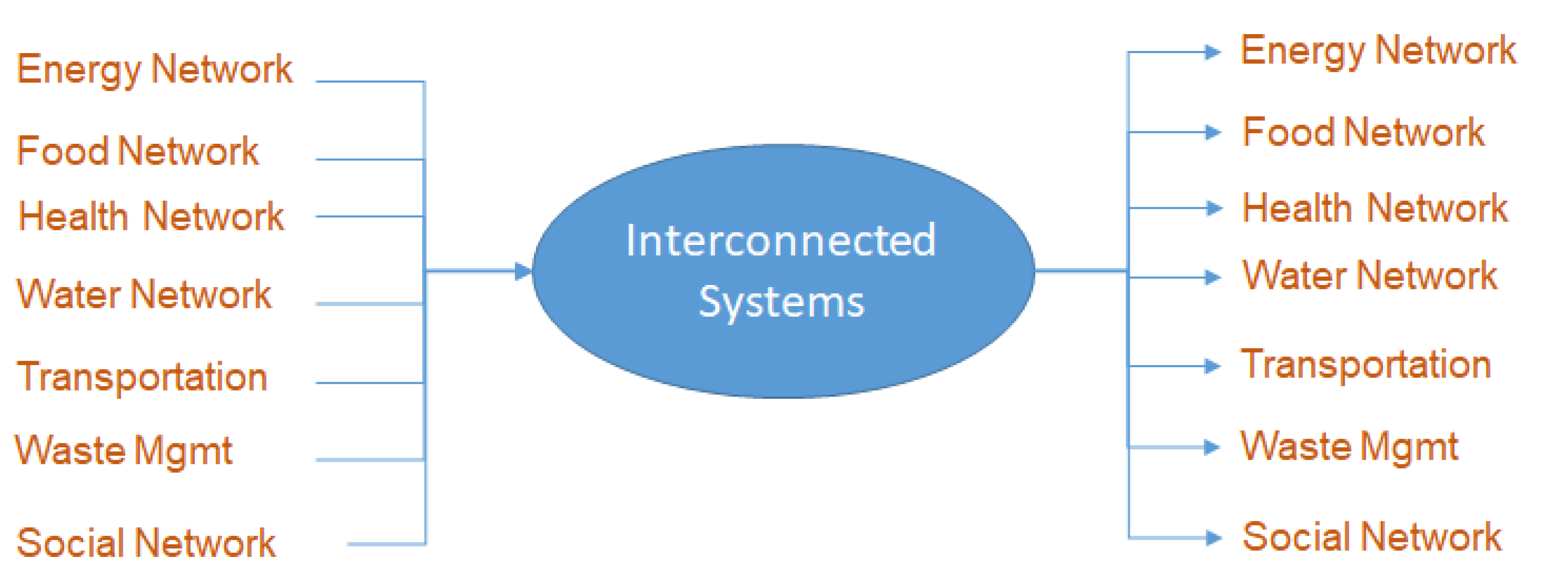
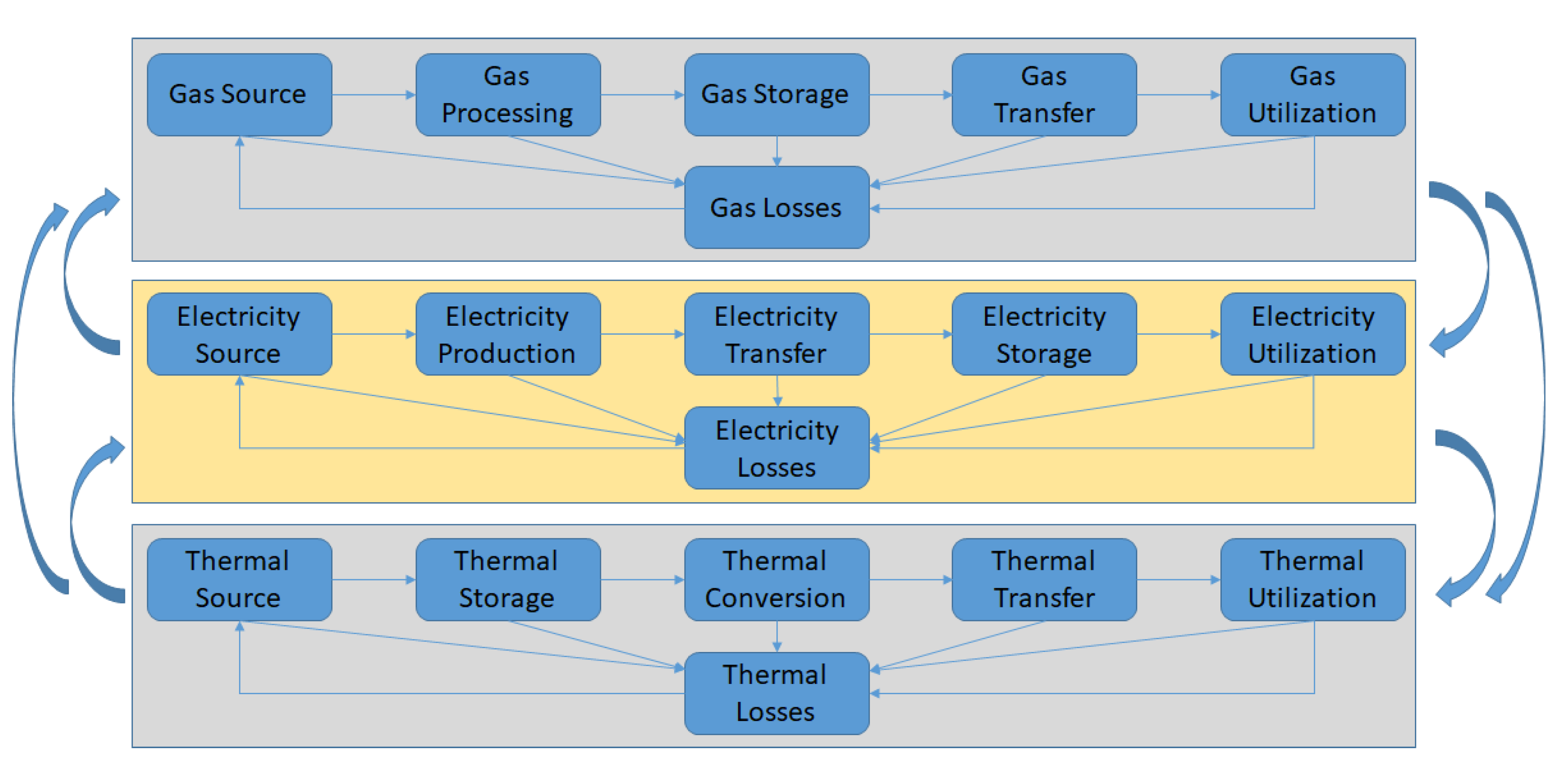
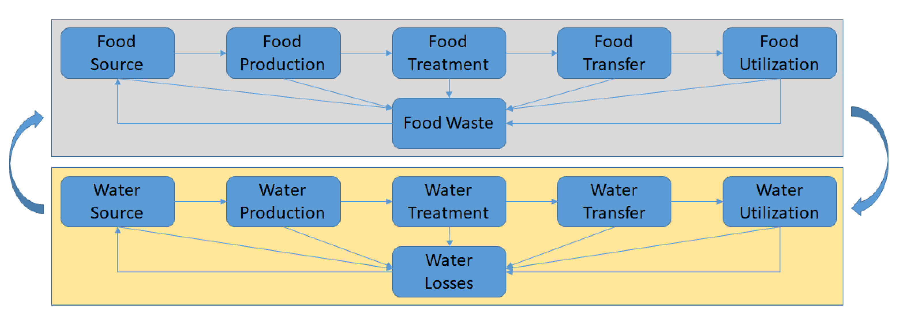
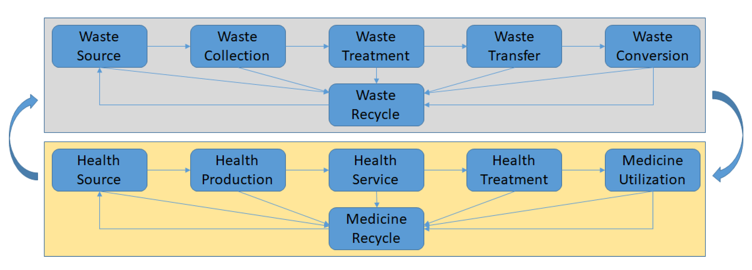
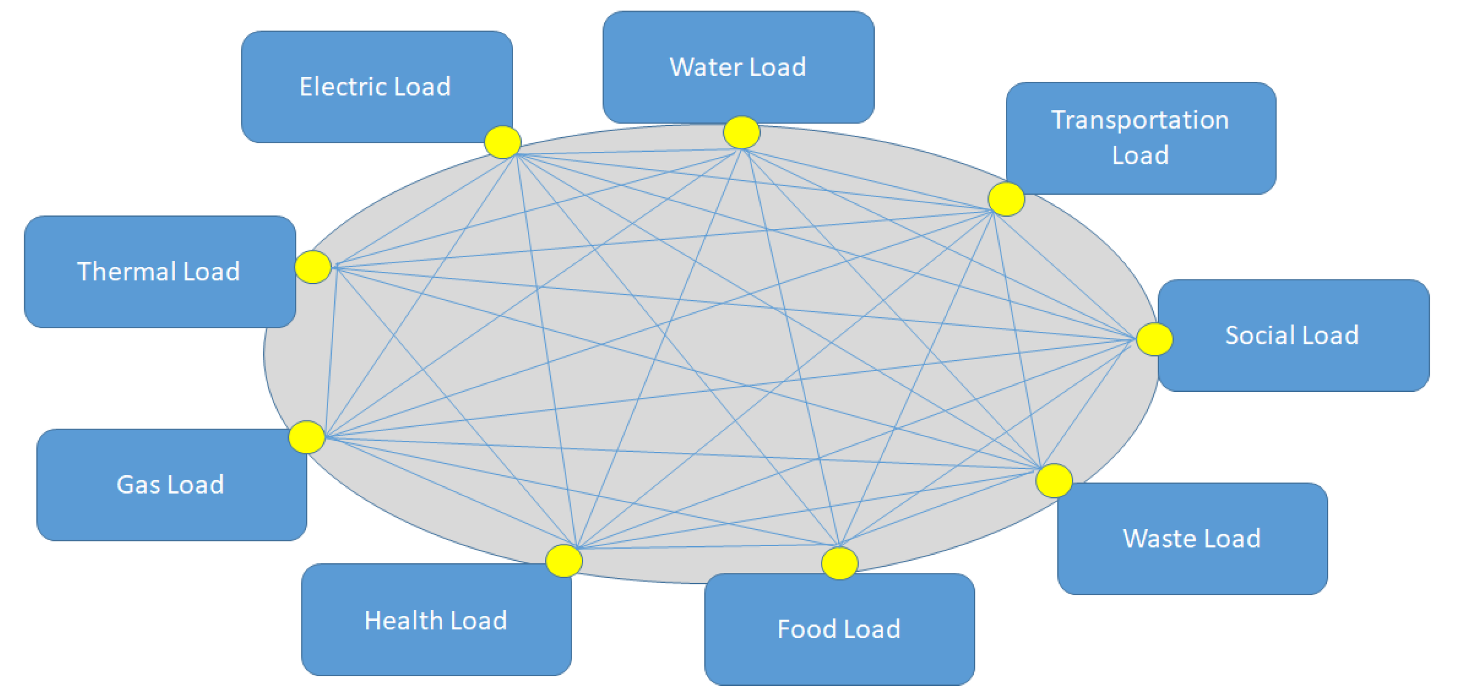
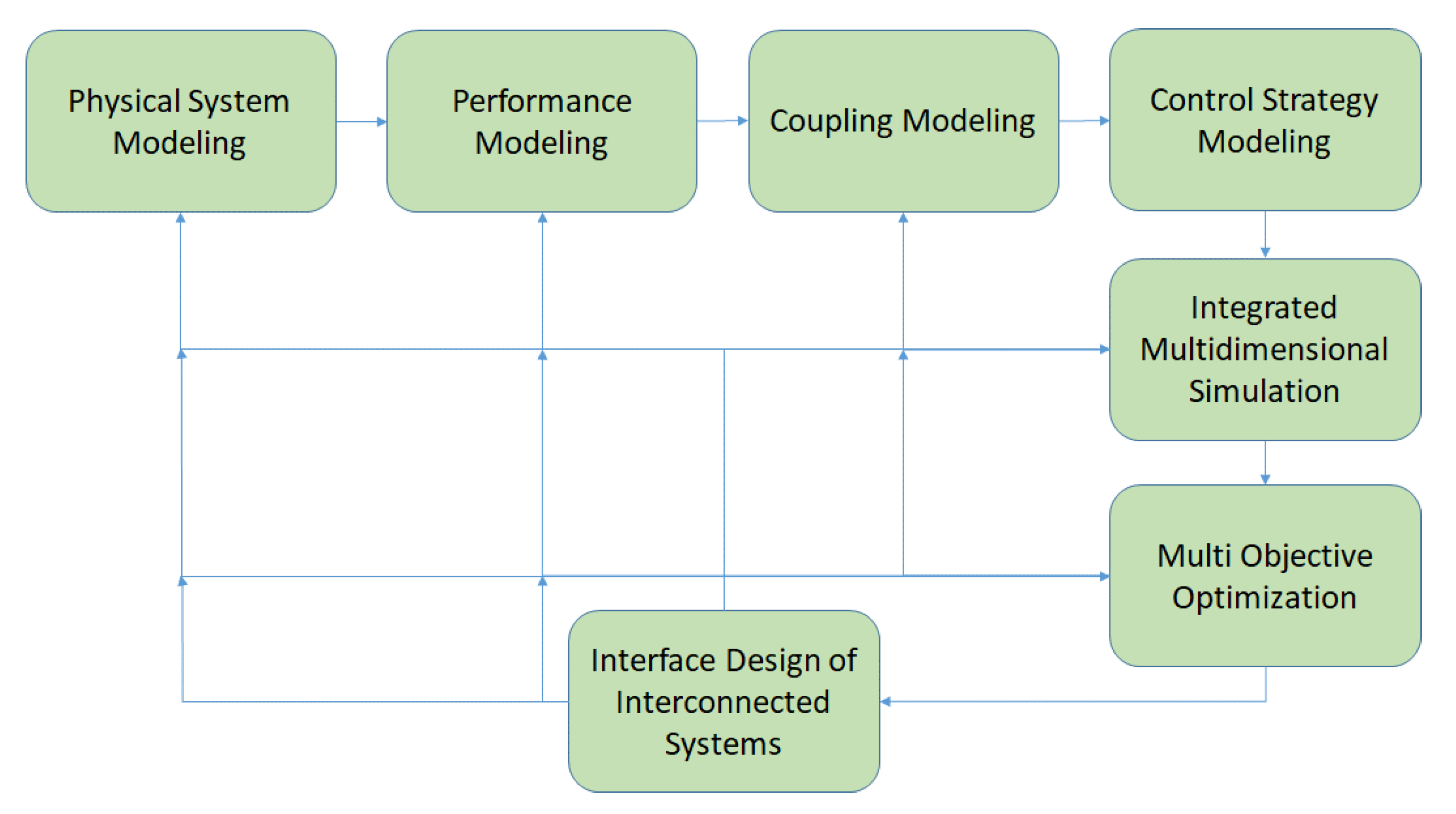
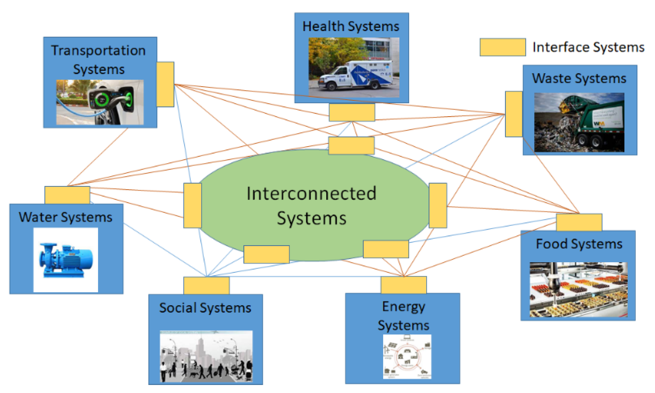
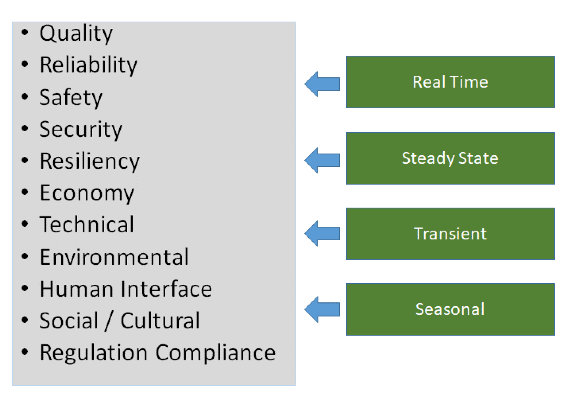
2. Interconnected System Modeling

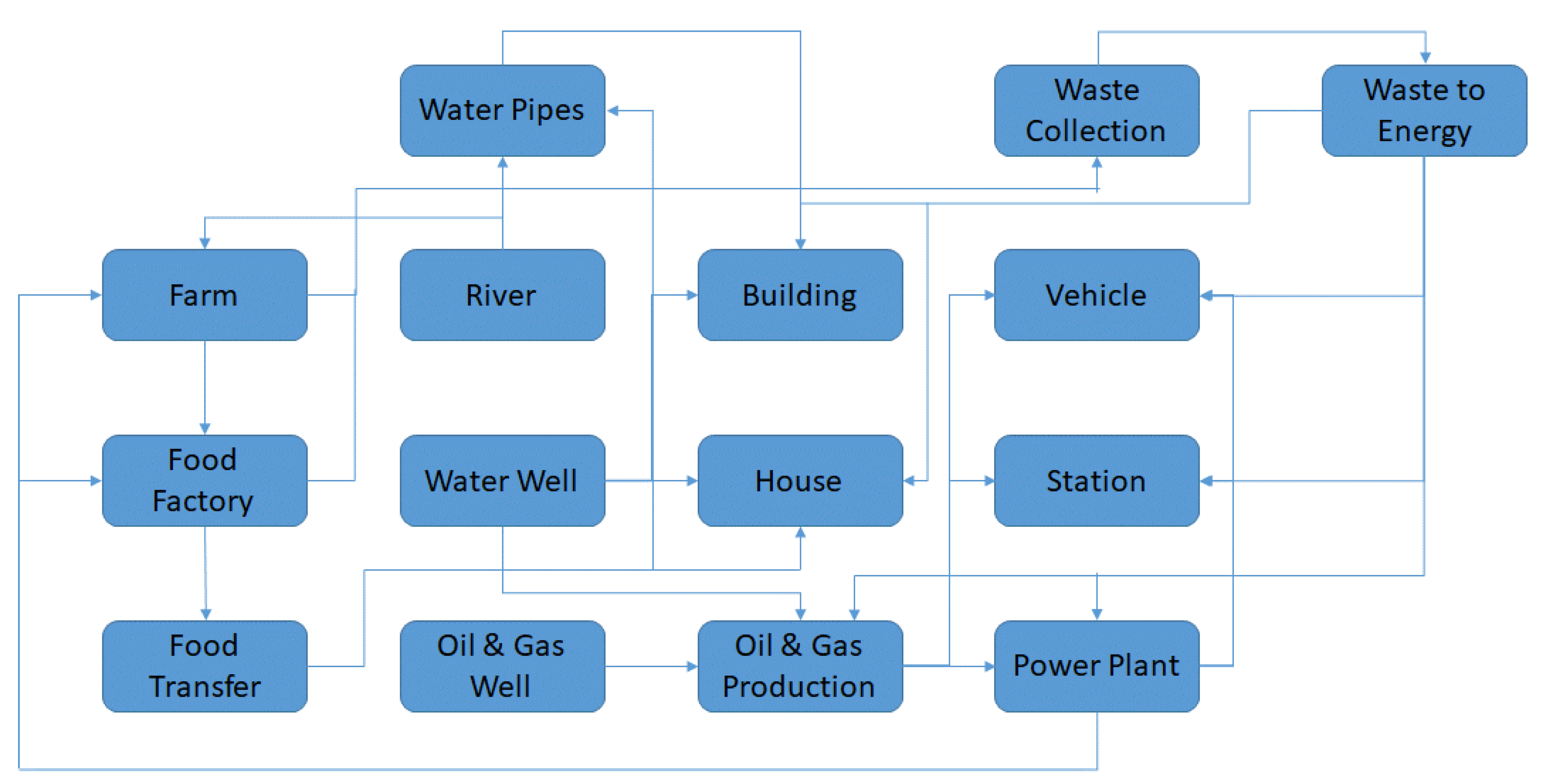
Smart cities are urban areas that utilize sensor networks with technological infrastructures to manage different activities and real-time data to achieve a flexible and high-performance quality of life. Smart cities can be viewed as interconnected systems to enable real-time interactions among different systems, processes, and infrastructures. To enable the engineering and management of these interactions, it is important to understand the possible dependencies and coupling among these systems and link them to design, control, and operation parameters. Examples of the possible couplings among these systems include hybrid energy systems (i.e., energy–transportation systems, energy–water systems, energy–food systems, energy–health systems, energy–waste systems, energy–social systems) and integration among any three or more of these systems. The proposed modeling of possible interactions among these systems can be represented by defining basic building blocks of each system. Energy systems can be expanded into gas-, electricity-, and thermal-related networks, along with the interactions among them. There are conversion strategies from gas to power, power to gas, thermal to gas, and other such combinations, linked to storage and utilization components. Figure 2 shows the interactions among electricity, thermal, and gas networks, where sources are linked to processing or production systems. These networks are linked with storage and transfer or transportation, as well as utilization. Losses are also modeled as linked to all these components within each system.

Similarly, the interconnections between food and water networks are modeled in Figure 3. The interconnection between waste and health networks are shown in Figure 4. The interactions among all these systems are clear by linking the different systems. In this figure, health sources could refer to medicine, natural herbal medicine, or healthcare technology. This is followed by the production and supply chain of these sources until they reach health services for treatment and medicine utilization, as well as possible recycling. Similarly, waste management systems start with waste sources, followed by collection, treatment and transfer/transportation, conversion, and possible recycle. There are interactions among these systems that require unified interfaces to enable the hybrid system modeling, engineering design, and control of the interconnected systems.

There are interactions among different loads, whereby an increase in one load might be related to factors that impact other loads. For example, gas load might increase due to activities that are directed toward gas supply with a slight reduction in electric load. Figure 5 shows possible interactions among all possible loads, including electric, thermal, gas, transportation, water, waste, food, health, and social loads. A better understanding of the coupling and interactions among these loads can lead to better energy conservation and management. Moreover, a better understanding of the behavior of interconnected systems can improve the overall mapping between energy supply and loads with enhanced performance of the developed hybrid energy systems.

3. Case Study

To understand a possible interconnected system, a case study is illustrated in Figure 6. It shows a food cycle involving the farm, food factory, and food transfer or transportation. This is linked to the water cycle, including rivers, water wells, and water pipes. The links to food utilization are represented by buildings and houses. This can be expanded to different residential areas. The waste cycle is also represented with waste collection systems and waste-to-energy conversion, which can be linked back to residential and industrial facilities and interfaces to the grid. Fuel sources start with oil and gas wells, followed by processing, production, and power plants to generate electricity and thermal byproducts, which are linked back to other infrastructures for energy utilization. This case study is only a snapshot of possible interactions among different components within interconnected systems, which illustrates the proposed solution. Transportation is represented with vehicles and stations so that it can be used for the transportation of food, social, water, and oil and gas.

The proposed model parameters are explained in

Table 1. Model parameters and key performance indicators of the case study interconnected systems.

System	Model Parameters	KPIs
Farm	Location: $F_L$ (latitude and longitude) Size: $F_S$ (square foot) Energy Demand: $F_E$ (kWh) Water Demand: $F_{Wtr}$ (${\mathrm{km}}^3$) Waste Generated: $F_{Wst}$ (tons)	Annual Yield: $F_Y$ (ton/year) Annual Waste: $F_{AWst}$ (ton/year) Annual Cost of Energy: $F_{ACE}$ ($/year) Annual Cost of Water: $F_{ACWtr}$ ($/year) Annual Energy Generated: $F_{EG}$ (kWh/year) Annual GHG Emissions: $F_{GE}$ (ton/year)
Food factory	Location: $D_L$ (latitude and longitude) Size: $D_S$ (square foot) Energy Demand: $D_E$ (kWh) Water Demand: $D_{Wtr}$ (${\mathrm{km}}^3$) Waste Generated: $D_{Wst}$ (tons)	Annual Yield: $D_Y$ (ton/year) Annual Waste: $D_{AWst}$ (ton/year) Annual Cost of Energy: $D_{ACE}$ ($/year) Annual Cost of Water: $D_{ACWtr}$ ($/year) Annual Energy Generated: $D_{EG}$ (kWh/year) Annual GHG Emissions: $D_{GE}$ (ton/year)
Food transfer	Region: $T_{L1L2}$ (latitude-1,2 and longitude-1,2) Distance: $T_D$ (km) Energy Demand: $T_E$ (kWh) Food Transferred: $T_{FT}$ (tons) Waste Generated: $T_{Wst}$ (tons)	Annual Yield: $T_Y$ (ton/km/year) Annual Waste: $T_{AWst}$ (ton/km/year) Annual Cost of Energy: $T_{ACE}$ ($/year) Annual Cost of Water: $T_{ACWtr}$ ($/year) Annual Energy Generated: $T_{EG}$ (kWh/year) Annual GHG Emissions: $T_{GE}$ (ton/year)
Water well	Location: $W_L$ (latitude and longitude) Size: $W_D$ (depth, m) Energy Demand: $W_E$ (kWh) Water Demand: $W_{Wtr}$ (${\mathrm{km}}^3$)	Annual Yield: $W_Y$ (${\mathrm{km}}^3$/year) Annual Cost of Energy: $W_{ACE}$ ($/year) Annual Cost of Water: $W_{ACWtr}$ ($/year) Annual Energy Generated: $W_{EG}$ (kWh/year)
River	Region: $R_{L1L2}$ (latitude 1, 2 and longitude 1, 2) Distance: $R_D$ (km) Size: $R_{WD}$ (width, depth, m) Water Flow: $R_{Wf}$ (cubic meter per second (cms)) River Ship Capacity: $R_{SC}$ (ships/h)	Annual Water Flow: $R_{WF}$ (${\mathrm{km}}^3$/year) Annual Transfer of Goods: $R_{ATG}$ (ton/year) Annual Ships: $R_S$ (ship/year) Annual Cost of Maintenance: $R_{ACM}$ ($/year) Annual GHG Emissions: $R_{GE}$ (ton/year)
Water pipe	Region: $P_{L1L2}$ (latitude-1,2 and longitude-1,2) Distance: $P_D$ (km) Size: $P_{WD}$ (diameter, depth, m) Water Flow: $R_{Wf}$ (cubic m per second (cms))	Annual Water Flow: $P_{WF}$ (${\mathrm{km}}^3$/year) Annual Cost of Maintenance: $P_{ACM}$ ($/year) Annual GHG Emissions: $R_{GE}$ (ton/year)
Building	Location: $B_L$ (latitude and longitude) Size: $B_S$ (square foot) Energy Demand: $B_E$ (kWh) Water Demand: $B_{Wtr}$ (${\mathrm{km}}^3$) Waste Generated: $B_{Wst}$ (tons)	Annual Occupancy: $B_O$ (occupant/year) Annual Waste Generate: $B_{AWst}$ (ton/year) Annual Cost of Energy: $B_{ACE}$ ($/year) Annual Cost of Water: $B_{ACWtr}$ ($/year) Annual Energy Generated: $B_{EG}$ (kWh/year) Annual GHG Emissions: $B_{GE}$ (ton/year)
House	Location: $H_L$ (latitude and longitude) Size: $H_S$ (square foot) Energy Demand: $H_E$ (kWh) Water Demand: $H_{Wtr}$ (${\mathrm{km}}^3$) Waste Generated: $H_{Wst}$ (tons)	Annual Occupancy: $H_O$ (occupant/year) Annual Waste Generate: $H_{AWst}$ (ton/year) Annual Cost of Energy: $H_{ACE}$ ($/year) Annual Cost of Water: $H_{ACWtr}$ ($/year) Annual Energy Generated: $H_{EG}$ (kWh/year) Annual GHG Emissions: $H_{GE}$ (ton/year)
Vehicle	Type: $V_E$ (engine size, L) Fuel: $V_F$ (L/100 km) Energy Demand: $V_E$ (kWh) Water Demand: $V_{Wtr}$ (${\mathrm{km}}^3$) GHG Emission: $V_{GE}$ (tons)	Annual Occupancy: $V_O$ (occupant/year) Annual Cost of Maintenance: $V_{ACM}$ ($/year) Annual Cost of Energy: $V_{ACE}$ ($/year) Annual Energy Generated: $V_{EG}$ (kWh/year) Annual GHG Emissions: $V_{GE}$ (ton/year)
Station	Location: $S_L$ (latitude and longitude) Size: $S_S$ (square meter) Vehicle Served: $S_V$ (vehicle/h) Energy Demand: $S_E$ (kWh) Water Demand: $S_{Wtr}$ (${\mathrm{km}}^3$) Waste Generated: $S_{Wst}$ (tons)	Annual Occupancy: $S_O$ (occupant/year) Annual Vehicle Served: $S_{AVS}$ (vehicle/year) Annual Waste Generated: $S_{AWst}$ (ton/year) Annual Cost of Energy: $S_{ACE}$ ($/year) Annual Cost of Water: $S_{ACWtr}$ ($/year) Annual Energy Generated: $S_{EG}$ (kWh/year) Annual GHG Emissions: $S_{GE}$ (ton/year)
Waste collection	Location: $Y_L$ (latitude and longitude) Size: $Y_S$ (cubic foot)	Annual Waste Collected: $Y_{AWst}$ (ton/year) Annual Cost of Maintenance: $Y_{ACM}$ ($/year)
Waste-to-energy	Location: $G_L$ (latitude and longitude) Size: $G_S$ (square meter) Energy Demand: $G_E$ (kWh) Water Demand: $G_{Wtr}$ (${\mathrm{km}}^3$) Energy Generated: $G_{EG}$ (kWh)	Annual Waste Generated: $G_{AWst}$ (ton/year) Annual Cost of Energy: $G_{ACE}$ ($/year) Annual Cost of Water: $G_{ACWtr}$ ($/year) Annual Energy Generated: $G_{EG}$ (kWh/year) Annual Cost of Maintenance: $G_{ACM}$ ($/year) Annual GHG Emissions: $G_{GE}$ (ton/year)
Oil and gas well	Location: $L_L$ (latitude and longitude) Size: $L_D$ (depth, m) Reservoir: $L_S$ (cubic meter)	Annual Yield: $L_Y$ (${\mathrm{km}}^3$/year) Annual Cost of Energy: $L_{ACE}$ ($/year) Annual Cost of Water: $L_{ACWtr}$ ($/year) Annual Energy Generated: $L_{EG}$ (kWh/year)
Oil and gas production	Location: $N_L$ (latitude and longitude) Size: $N_S$ (square foot) Energy Demand: $N_E$ (kWh) Water Demand: $N_{Wtr}$ (${\mathrm{km}}^3$) Oil/Gas Produced: $N_{OGP}$ (${\mathrm{km}}^3$)	Annual Production: $N_P$ (${\mathrm{km}}^3$/year) Annual Cost of Energy: $N_{ACE}$ ($/year) Annual Cost of Maintenance: $N_{ACM}$ ($/year) Annual Cost of Water: $N_{ACWtr}$ ($/year) Annual Energy Generated: $N_{EG}$ (kWh/year)
Power plant	Location: $Z_L$ (latitude and longitude) Size: $Z_S$ (square foot) Energy Demand: $Z_E$ (kWh) Water Demand: $Z_{Wtr}$ (${\mathrm{km}}^3$) Energy Generated: $Z_{EG}$ (kWh)	Annual Waste Generated: $Z_{AWst}$ (ton/year) Annual Cost of Energy: $Z_{ACE}$ ($/year) Annual Cost of Water: $Z_{ACWtr}$ ($/year) Annual Energy Generated: $Z_{EG}$ (kWh/year) Annual Cost of Maintenance: $Z_{ACM}$ ($/year) Annual GHG Emissions: $Z_{GE}$ (ton/year)

, which shows a list of key design, control, and operation parameters and performance measures used to analyze the interconnected systems.

Figure 7 shows more details regarding the interfaces among microgrid (MG), water facility, waste-to-energy facility, and EV charging station. It shows different levels of interfaces for integrated systems, connected systems, and autonomous systems. In principle, the integrated systems offer one direction of interfaces, at specific integration points, with local decision making or at a central point in the whole system. The connected systems offer two directions of interfaces with local and mutual decision making among connected systems. The autonomous systems offer two or multiple interface points with local decision making, while some decisions are assisted at the central or distributed levels.

The logic behind the universal interface design is described in Figure 8a,b, which shows the mechanism followed in the unified interface design, starting from health concerns. If any concern is identified from the health interface port, a resolution is needed on the basis of other parameters and logic followed in the control design. This is followed by environmental, social, material, water, electricity, gas, thermal, transport, data, and policy. Each model library defines the local parameters and constraints that can be linked to all available interfaces for local decision making on the basis of autonomous functions.

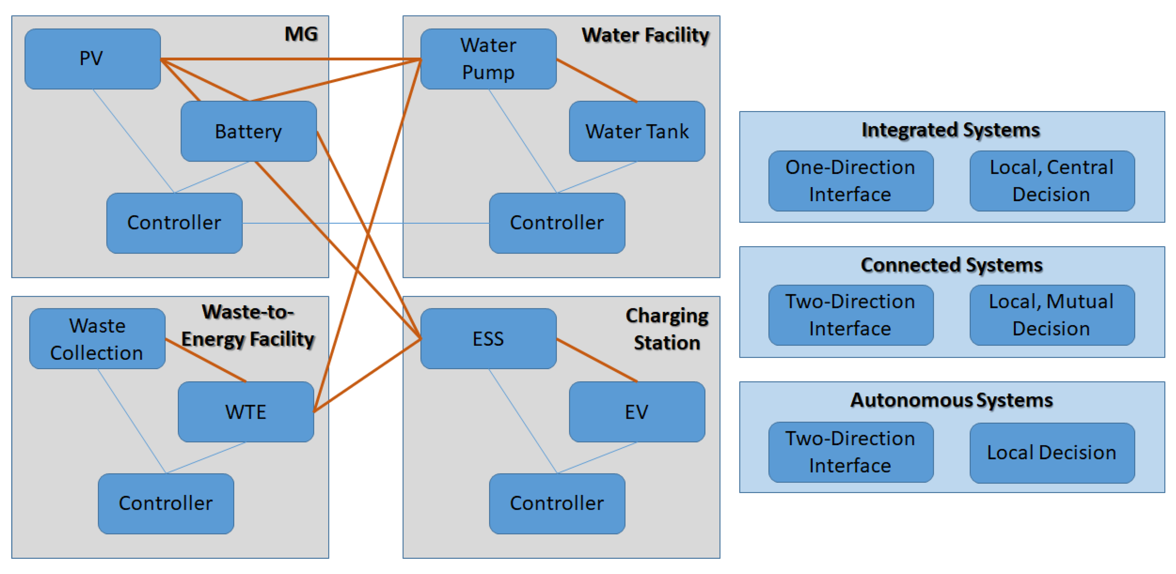
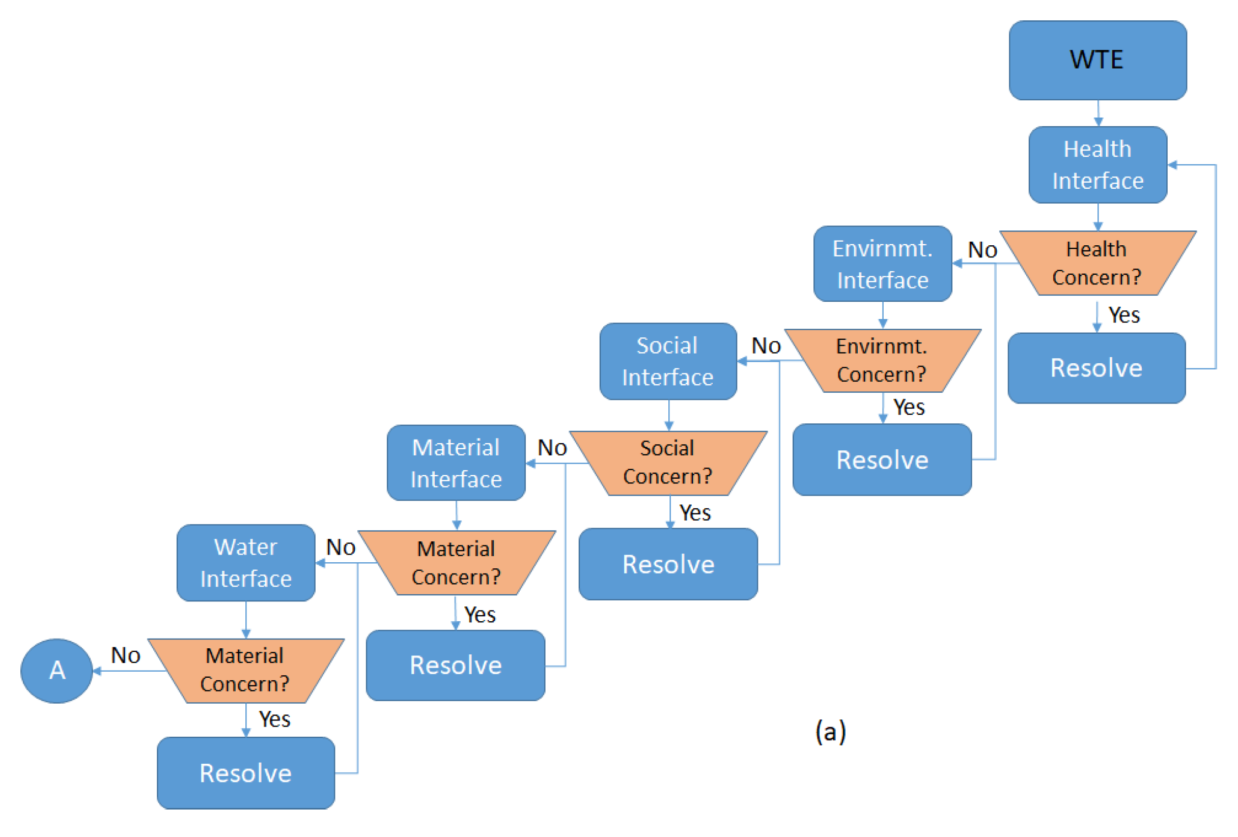
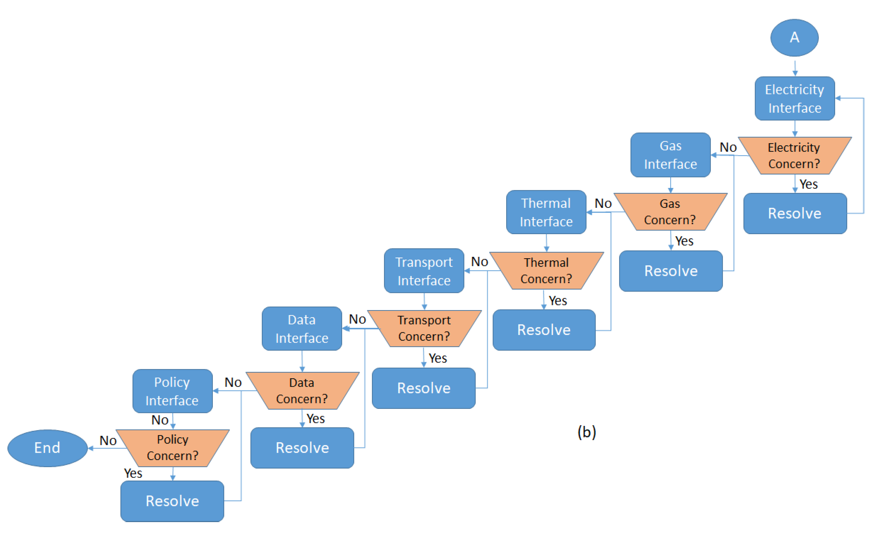
4. Unified Interface Modeling

To support the engineering design, control, and operation of such interface systems, it is essential to design a unified interface system that can enable modular interactions among interconnected systems with the systematic association among model parameters and KPIs. The proposed engineering design framework of the design of the unified interfaces of interconnected systems is shown in Figure 9. The physical system modeling can formulate the design, control, and operation parameters of each building block of each system.

This is followed by performance modeling of KPIs of each component and system. The different coupling mechanisms and parameters are defined, and equations are synthesized to identify dependencies among model parameters. According to the proper coupling among systems, control strategies can be defined for each system and evaluated with multidimensional simulations, using multiphysics capabilities to model thermal, electricity, gas, water, waste, transportation, food, health, and social. This is followed by multi-objective optimization to achieve the highest performance in each system and globally for the overall interconnected systems. The interface system design to coordinate different process variables and KPIs among model libraries can be defined for each system to enable the communication of process parameters for control and operation of the interconnected systems.

To better understand how the interface systems are designed and operated among interconnected systems, Figure 10 shows one example of interconnected systems, where the yellow box represents the unified interface system. The design of the input–output parameters and their utilizations in an engineering design example are explained in the next section.

To analyze more interface examples, it is essential to expand each network. Different components within the environmental system are listed, such as air, soil, water bodies, and lands. Similarly, components are listed within physical infrastructures such as buildings, roads, bridges, and hospitals. The interactions among these systems are established via interface systems, which can support integration and management. Similarly, components within the transportation networks are highlighted, including vehicles, stations, fueling and charging stations, and marine ships.

A detailed unified interface system design is described using standardized functions, from “F1” to “F10”, which are mapped to different dimensions, as shown in Figure 11. Two examples are illustrated using a vehicle, building, water pump, and machine. The understanding of these examples can facilitate the design of other components and systems.

The evaluation of different operation scenarios can be conducted on the basis of possible KPIs, as shown in Figure 12. The evaluation of different KPIs can be performed for design and operation scenarios as part of the simulation environment for real-time, steady-state, transient, and seasonal analysis. The list of functions is explained in

Table 2. Unified interface system design: functions and parameters.

Function	Parameters	KPIs
F1: Health Interface	F1.SV1: input medicine F1.SV2: input health services F1.SV3: output medicine F1.SV4: output health services F1.SV5: infectious diseases	F1.KPI1: health Index F1.KPI2: annual produced medicine F1.KPI3: annual consumed medicine F1.KPI4: annual healthcare served persons F1.KPI5: annual infection rate F1.KPI6: annual death rate F1.KPI7: annual recovery rate
F2: Material Interface	F2.SV1: input material mass F2.SV2: output material mass	F2.KPI1: annual GHG emissions F2.KPI2: annual material losses F3.KPI3: annual material processing costs
F3: Electricity Interface	F3.SV1: input current F3.SV2: input voltage F3.SV3: output current F3.SV4: output current F3.SV5: AC or DC	F3.KPI1: power factor F3.KPI2: power losses F3.KPI3: safety index F3.KPI4: risk index
F4: Gas Interface	F4.SV1: input gas flow F4.SV2: input gas type F4.SV3: output gas flow F4.SV4: output gas type F4.SV5: gas production capacity F4.SV6: gas energy conversion factor	F4.KPI1: annual gas production F4.KPI2: annual gas consumption F4.KPI3: gas processing exergy index F4.KPI4: annual GHG emissions F4.KPI5. annual processing costs
F5: Thermal Interface	F5.SV1: input thermal energy F5.SV2: output thermal energy F5.SV3: thermal power cycle F5.SV4: thermal efficiency F5.SV5: thermal storage capacity	F5.KPI1: annual thermal production F5.KPI2: annual thermal consumption F5.KPI3. annual thermal processing costs
F6: Environment Interface	F6.SV1: air contaminants F6.SV2: soil contaminants F6.SV3: water contaminants F6.SV4: water areas F6.SV5: occupants	F6.KPI1: air quality index F6.KPI2: lifecycle index F6.KPI3: sustainability index F6.KPI4: annual GHG emissions
F7: Water Interface	F7.SV1: water flow F7.SV2: water contents F7.SV3: water storage	F7.KPI1: annual water usage F7.KPI2: annual water loss F7.KPI3: annual water flow F7.KPI4: annual water storage
F8: Transport Interface	F8.SV1: transport capacity F8.SV2: transport speed F8.SV3: transport delays F8.SV4: transport type	F8.KPI1: annual transport capacity F8.KPI2: annual transport delays F8.KPI3: annual transport cost
F9: Data Interface	F9.SV1: data transfer rate F9.SV2: data storage F9.SV3: data access users	F9.KPI1: annual data transfer F9.KPI2: annual data storage F9.KPI3: annual data access users
F10: Social Interface	F10.SV1: local population F10.SV2: number of interactions F10.SV3: number of groups F10.SV4: number per gender	F10.KPI1: annual interactions F10.KPI2: annual interaction groups F10.KPI3: annual interactions gender ratio
F11: Policy	F11.SV1: policy function coverage % F11.SV2: number of related policies	F11.KPI1: % compliance with policy F11.KPI2: system performance as per policy

, where sample parameters for each function are illustrated for the defined 11 groups of possible interfaces with any component. The unified interface systems can systematically enable the analysis and engineering design and control of interconnected systems.

Table 3. Standards related to interfaces of interconnected systems.

P11—Standard for Rotating Electric Machinery for Rail and Road Vehicles [29]

CSA standards for Water Pumps (CAN/CSA-C22.2 No. 108-01) [30]

CSA standards for Thermal Devices (CSA C22.2 NO 130) [31]

CSA standards for Fuel Devices (CSA C22.2 NO 3) [32]

CSA Standard for Control equipment (CSA C22.2 NO 14) [33]

IEEE 1636-2009—IEEE Standard for Software Interface for Maintenance Information Collection and Analysis (SIMICA) [34]

provides a list can possible related standards that reflect interfaces in different equipment, which will be used to evaluate the compliance and interactions among interconnected systems.

5. Analysis of Unified Interface System Implementation

The proposed unified interface system was applied to interconnected systems shown in the case study used with several scenarios, as shown in

Table 4. Scenario details applied to the case study.

Scenario	Transportation of Food via Vehicle from Point A to Point B
Parameter Changes	SO1: Change vehicle type: (a) gas vs. (b) electric SO2: Change route: (a) use highway vs. (b) use the shortest path Factors: Food and material process, transport, cost, energy conversion Environmental performance, GHG emissions Transportation performance, mobility, vehicle technology, delay, cost Social interactions, gender Gas process, losses, cost, supply chain Data and knowledge sharing

.

Scenario Details: In this scenario, food was transported from point A to point B via a vehicle. The datasets involved in this scenario are represented in

Table 5. Scenario details of transportation of food via vehicle from point A to point B.

Point A	43.92258120910123, −79.3780351047355
Point B	43.900545798084586, −79.26182245727405
Distance	14.3 km
Interface parameters	F2.SV1: input material/food mass: 500 kg F2.SV2: output material mass: 480 kg F4.SV2: input gas type: gasoline F4.SV3: output gas flow: 8.0 L/100 km F4.SV4: output gas type: gasoline F4.SV5: gas production capacity: 0 F4.SV6: gas production efficiency: 80% F6.SV1: air contaminants: CO2 F6.SV2: soil contaminants: n/a F6.SV3: water contaminants: n/a F6.SV4: water areas: n/a F6.SV5: occupants: 2 persons F8.SV1: transport capacity: 2 persons F8.SV2: transport speed: 80 km/h F8.SV3: transport delays: 1 h/100 km F10.SV1: local population: 150,000 persons, based on comparative region population F10.SV2: number of interactions: 10/trip, based on average interactions during last year F10.SV3: number of groups: 4 (goods transport, food safety, food market, supermarket chain), based on a selected sample from the identified region F10.SV4: gender ratio, based on selected sample

. In this scenario, input and output material/food mass were defined for a trip and evaluated in view of the defined KPIs within selected groups. The analysis shows the importance of the defined KPIs, and how they could be used to evaluate interconnected systems.

Transportation emissions data have been analyzed in several countries, including the USA [34,35]. EV-related emission data on different road types were described in [36], while truck data were presented in [36,37]. A comparison of vehicle, fuel, and use regarding GHG was also analyzed in [38,39,40,41,42].

Greenhouse Gas (GHG) emissions = D × W × EF,

(1)

where D is the distance of shipping in miles or kilometers, W is the weight or amount of shipment in pounds, kilograms, or tons, or volume metrics such as 20 foot equivalent unit (TFEs), and EF is the emission factor.

The estimated GHG as per Equation (1) was used to estimate related performance measures, as shown in

Table 6. Scenario variations based on selected options (standardized).

KPI	KPI Value
F2.KPI1: annual GHG emissions	15 kg
F2.KPI2: annual material losses	400 kg
F3.KPI3: annual material processing costs	$400,000
F4.KPI1: annual gas production	n/a
F4.KPI2: annual gas consumption	580 L
F4.KPI3: gas processing exergy index	n/a
F4.KPI5: annual processing costs	$760
F6.KPI1: air quality index	70%
F6.KPI2: lifecycle index	60%
F6.KPI3: sustainability index	75%
F8.KPI1: annual transport capacity	450,000 kg
F8.KPI2: annual transport delays	270
F8.KPI3: annual transport cost	36,000
F10.KPI1: annual interactions	1800
F10.KPI2: annual interaction groups	72
EV (Ford Focus)
Within city roads	110 MPGe [42]
Highway roads	99 MPGe [43]
Within city roads	30 MPG
Highway roads	40 MPG
Annual GHG emission of carbon dioxide per kilowatt-hour of battery capacity (kg CO2/kWh) for electric vehicles	56 to 494 kg [37]
Gasoline GHG emissions of CO2/ton-mile	161.8 g [38]
Annual transport cost for EV in the United States	$485 [40]
Annual transport cost for gasoline car in the United States	$1117 [40]

. The evaluations of the selected KPIs were estimated for the defined scenarios, which showed an air quality index of 70%, sustainability index of 75%, and lifecycle index of 60%. This is expected to improve KPIs with variations of the related scenario parameters such as gas consumption, gas production, transportation loads, and other related parameters through the interfaces defined with the 11 groups. This is useful to enable improving the performance of the target integrated system. In addition, it can enhance the overall performance of the interconnected systems. On the social side and to achieve diversity across system functions, other factors such as sustainability, economy, environment, and energy could be studied using the interfaces with the social function and gender groups. The proposed model could be used to enhance the performance of energy, transportation, traffic, water, food, waste treatment, health, and social networks.

The analysis of these performance measures led to a better understanding of the impacts of different model parameters within the different domains, such as energy, transportation, and environment. The overall performance can be optimized on the basis of user preference weights of these KPIs using multi-objective optimization algorithms, which will be described in future work.

6. Conclusions

The world is moving toward smart cities, where systems and components are individually designed and operated as smart nodes in complex interconnected systems. There is a lack of best practices for achieving the engineering design of interconnected systems. This paper presented a holistic framework of the engineering design of interconnected systems, including energy, water, transportation, waste, environment, food, health, and social networks. The interactions among these systems require unified interface systems to analyze the multidimensional views of these interconnected systems. A generic framework was presented with the analysis of multiple scenarios applied to a selected case study. The concept of optimization was discussed in view of infrastructures and associated key performance indicators defined for each dimension and system. The presented work will be extended to provide multi-objective optimization with real-time links to the multidimensional simulation of interconnected systems. There are limitations regarding the possible ways to model interconnected systems where the interface points are not adequately understood. Existing approaches such as multidimensional modeling of integrated systems are able to map model parameters in different domains and build relationships among them. However, these approaches are not able to model the coupling information and interactions among different systems. The proposed approach is able to cover these gaps and build standardized interactions based on unified interfaces that are generalized for each system. KPIs are also mapped to these interface points to enable the evaluation of all design and operation parameters for different scenarios and control strategies, thus supporting real time performance optimization and leading to profitable implementation and deployment.

Further studies are required to investigate the detailed design of practical interfaces and multiphysics models to accurately represent interconnected systems. More case studies will be analyzed using the presented hybrid modeling approach of interconnected systems. The further development of examples will support expanding the proposed approach to several applications, which will help the transition toward smart cities.

References

1. UN World Population Prospects: The 2017 Revision; Population Division, Department of Economic and Social Affairs, United Nations: New York, NY, USA, 2017.
2. Kaundinya, D.P.; Balachandra, P.; Ravindranath, N.H. Grid-connected versus stand-alone energy systems for decentralized power—A review of literature. Renew. Sustain. Energy Rev. 2009, 13, 2041–2050. [Google Scholar] [CrossRef]
3. Erdinc, O.; Uzunoglu, M. Optimum design of hybrid renewable energy systems: Overview of different approaches. Renew. Sustain. Energy Rev. 2012, 16, 1412–1425. [Google Scholar] [CrossRef]
4. Levina, T.; Thomas, V.M. Least-cost network evaluation of centralized and decentralized contributions to global electrification. Energy Policy 2012, 41, 286–302. [Google Scholar] [CrossRef]
5. Ma, T.; Wu, J.; Hao, L.; Lee, W.; Yan, H.; Li, D. The optimal structure planning and energy management strategies of smart multi energy systems. Energy 2018, 160, 122–141. [Google Scholar] [CrossRef]
6. Shabanpour-Haghighi, A.; Seif, A.R. Effects of district heating networks on optimal energy flow of multi-carrier systems. Renew. Sustain. Energy Rev. 2016, 59, 379–387. [Google Scholar] [CrossRef]
7. Rastegar, M.; Fotuhi-Firuzabad, M. Load management in a residential energy hub with renewable distributed energy resources. Energy Build. 2015, 107, 234–242. [Google Scholar] [CrossRef]
8. Mohammadia, M.; Noorollahia, Y.; Mohammadi-ivatloo, B.; Hosseinzadehc, M.; Yousefia, H.; Khorasani, S.T. Optimal management of energy hubs and smart energy hubs—A review. Renew. Sustain. Energy Rev. 2018, 89, 33–50. [Google Scholar] [CrossRef]
9. Lund, H.; Andersen, A.N.; Østergaard, P.A.; Mathiesen, B.V.; Connolly, D. From electricity smart grids to smart energy systems e A market operation based approach and understanding. Energy 2012, 42, 96–102. [Google Scholar] [CrossRef]
10. Lund, H.; Østergaard, P.A.; Connolly, D.; Mathiesen, B.V. Smart energy and smart energy systems. Energy 2017, 137, 556–565. [Google Scholar] [CrossRef]
11. Abedi, S.; Alimardani, A.; Gharehpetian, G.B.; Riahy, G.H.; Hosseinian, S.H. A comprehensive method for optimal power management and design of hybrid RES-based autonomous energy systems. Renew. Sustain. Energy Rev. 2012, 16, 1577–1587. [Google Scholar] [CrossRef]
12. Nasiakou, A.; Vavalis, M.; Zimeris, D. Smart energy for smart irrigation. Comput. Electron. Agric. 2016, 129, 74–83. [Google Scholar] [CrossRef]
13. Pazouki, S.; Haghifam, M.R. Optimal planning and scheduling of energy hub in presence of wind, storage and demand response under uncertainty. Electr. Power Energy Syst. 2016, 80, 219–239. [Google Scholar] [CrossRef]
14. Wasilewski, J. Integrated modelling of microgrid for steady-state analysis using the modified concept of a multi-carrier energy hub. Electr. Power Energy Syst. 2015, 73, 891–898. [Google Scholar] [CrossRef]
15. Wang, Y.; Cheng, J.; Zhang, N.; Kang, C. Automatic and linearized modeling of energy hub and its flexibility analysis. Appl. Energy 2018, 211, 705–714. [Google Scholar] [CrossRef]
16. Maśloch, P.; Maśloch, G.; Kuźmiński, Ł.; Wojtaszek, H.; Miciuła, I. Autonomous Energy Regions as a Proposed Choice of Selecting Selected EU Regions—Aspects of Their Creation and Management. Energies 2020, 13, 6444. [Google Scholar] [CrossRef]
17. Belleville, M.; Fanet, H.; Fiorini, P.; Nicole, P.; Pelgrom, M.J.M.; Piguet, C.; Hahn, R.; van Hoof, C.; Vullers, R.; Tartagni, M.; et al. Energy autonomous sensor systems: Towards a ubiquitous sensor technology. Microelectron. J. 2010, 41, 740–745. [Google Scholar] [CrossRef]
18. Bieber, N.; Ker, J.H.; Wang, X.; Triantafyllidis, C.; van Dam, K.H.; Koppelaar, R.H.E.M.; Shah, N. Sustainable planning of the energy-water-food nexus using decision-making tools. Energy Policy 2018, 113, 584–607. [Google Scholar] [CrossRef]
19. Barbosa, A.; Martín, B.; Hermoso, V.; Arévalo-Torres, J.; Barbière, J.; Martínez-López, J.; Domisch, S.; Langhans, S.D.; Balbi, S.; Villa, F.; et al. Cost-effective restoration and conservation planning in Green and Blue Infrastructure designs. A case study on the Intercontinental Biosphere Reserve of the Mediterranean: Andalusia (Spain)—Morocco. Sci. Total Environ. 2019, 652, 1463–1473. [Google Scholar] [CrossRef]
20. Simpson, G.B.; Jewitt, G.P.W. The development of the water-energy-food nexus as a framework for achieving resource security: A review. Front. Environ. Sci. 2019, 7, 8. [Google Scholar] [CrossRef] [Green Version]
21. Alzard, M.H.; Maraqa, M.A.; Chowdhury, R.; Khan, Q.; Albuquerque, F.D.B.; Mauga, T.I.; Aljunadi, K.N. Estimation of Greenhouse Gas Emissions Produced by Road Projects in Abu Dhabi, United Arab Emirates. Sustainability 2019, 11, 2367. [Google Scholar] [CrossRef] [Green Version]
22. Marcilio, G.P.; Rangel, J.J.; de Souza, C.L.M.; Shimoda, E.; da Silva, F.F.; Peixoto, T.A. Analysis of greenhouse gas emissions in the road freight transportation using simulation. J. Clean. Prod. 2018, 170, 298–309. [Google Scholar] [CrossRef]
23. United States Environmental Protection Agency (US EPA). MOVES2014a: Latest Version of Motor Vehicle Emission Simulator (MOVES). Available online: https://www.epa.gov/moves/moves2014a-latest-versionmotor-vehicle-emission-simulator-moves (accessed on 3 September 2017).
24. United States Department of Energy (US DoE). Method for Calculating Carbon Sequestration by Trees in Urban and Suburban Settings; U.S. Department of Energy: Washington, DC, USA, 1998.
25. Biggs, E.M.; Bruce, E.; Boruff, B.; Duncan, J.M.A.; Horsley, J.; Pauli, N.; McNeill, K.; Neef, A.; Van Ogtrop, F.; Curnow, J.; et al. Sustainable development and the water-energy-food nexus: A perspective on livelihoods. Environ. Sci. Policy 2015, 54, 389–397. [Google Scholar] [CrossRef] [Green Version]
26. Smith, K.; Liu, S.; Liu, Y.; Guo, S. Can China reduce energy for water? A review of energy for urban water supply and wastewater treatment and suggestions for change. Renew. Sustain. Energy Rev. 2018, 91, 41–58. [Google Scholar] [CrossRef]
27. Helmdach, D.; Yaseneva, P.; Heer, P.K.; Schweidtmann, A.M.; Lapkin, A. A Multiobjective Optimization Including Results of Life Cycle Assessment in Developing Biorenewables-Based Processes. ChemSusChem 2017, 10, 3632–3643. [Google Scholar] [CrossRef] [PubMed]
28. Vadenbo, C.; Hellweg, S.; Guillén-Gosálbez, G. Multi-objective optimization of waste and resource management in industrial networks—Part I: Model description Resources, conservation and recycling. Resour. Conserv. Recycl. 2014, 89, 52–63. [Google Scholar] [CrossRef]