Abstract
Accurate electricity demand forecasting for a short horizon is very important for day-to-day control, scheduling, operation, planning, and stability of the power system. The main factors that affect the forecasting accuracy are deterministic variables and weather variables such as types of days and temperature. Due to the tropical climate of Thailand, the marginal impact of weather variables on electricity demand is worth analyzing. Therefore, this paper primarily focuses on the impact of temperature and other deterministic variables on Thai electricity demand. Accuracy improvement is also considered during model design. Based on the characteristics of demand, the overall dataset is divided into four different subgroups and models are developed for each subgroup. The regression models are estimated using Ordinary Least Square (OLS) methods for uncorrelated errors, and General Least Square (GLS) methods for correlated errors, respectively. While Feed Forward Artificial Neural Network (FF-ANN) as a simple Deep Neural Network (DNN) is estimated to compare the accuracy with regression methods, several experiments conducted for determination of training length, selection of variables, and the number of neurons show some major findings. The first finding is that regression methods can have better forecasting accuracy than FF-ANN for Thailand’s dataset. Unlike much existing literature, the temperature effect on Thai electricity demand is very interesting because of their linear relationship. The marginal impacts of temperature on electricity demand are also maximal at night hours. The maximum impact of temperature during night hours happens at 11 p.m., is 300 MW/C, about rise in demand while during day hours, the temperature impact is only 10 MW/C to 200 MW/C about to rise.
1. Introduction
1.1. Motivation and Background
Thailand has 100% access to electricity [1] for both urban and rural areas with the second-largest economy and the fourth-largest country by population in Southeast Asia. Such population and the economic growth lead to an increment of electricity demand by an annual average of 684 MW since 1987 [2]. Among Asian countries, the People’s Republic of China (PRC) accounts for most of the energy demand in Asia whereas Thailand stands in the fifth followed after India, Korea, and Indonesia [3]. The Electric Supply Industry of Thailand consists of Electricity Generating Authority of Thailand (EGAT), Metropolitan Electricity Authority (MEA), and Provincial Electricity Authority (PEA); where EGAT is responsible for generation, MEA for distribution in the metropolitan area around Bangkok, and PEA distribution in the rest of the country. The scope of our paper is centered on the metropolitan areas.
Short-term electricity demand load forecasting has become an extremely important issue for energy suppliers, system operators, and other market participants. In many electricity deregulated markets, around the world electricity demand is fixed a day before the delivery by concurrent (semi-)hourly auctions. The improved accuracy of demand load forecasting can save the operating cost and the reliability of power supply. The volatile and complex behavior of electricity demand is always a challenging task when developing robust models for the researcher. Smart technologies like the internet of things, need sufficient power to connects “anything from anywhere” [4]. Industry automation and large penetration of plug-in electric vehicles are expected for reliable, economically competitive, environmentally sustainable electric system [4,5]. The fifth assessment report of the Intergovernmental Panel on Climate Change [6] suggested that global warming already made the world 0.74 C warmer and forecasted to 1.8–4 C by the end of century [7,8,9]. This increment in temperature has already shifted the highest peak demand load occurrence from evening hours to daytime hours due to the intensive use of the air conditioning (AC) systems in Jordan [7]. The outside temperature is demonstrated as the most influencing factor among all the variables that can be used to explain potential variations in demand [10,11]. Furthermore, this influence is typically linked to the penetration of electric cooling and heating appliances, mainly used by households and firms in residential and commercial sectors [11]. Heating, ventilation, and the AC system consume more than half of energy in the buildings of residential area [12]. In addition to temperature, deterministic variables such as day types and seasons also show their impacts on demand. The behavior of demand is highly dependent on the sectors where the electricity is used. The influence of residential sector behavior on energy consumption is getting increasingly significant [13]. Since the electricity cannot be stored efficiently, end-user demand must be tightly controlled for an effective power system management [14]. Therefore, the main objective of this article is to construct an accurate forecasting model, and quantitative analysis of demand load influencing factors that help to ensure the stability of the energy system in operation, maintain the secure, adequate, and efficient electricity supply by reducing blackout risk. To avoid an ambiguous presentation, we note that the rest of this paper uses two terms, “demand forecasting” and “demand” to refer to “electricity demand forecasting” and “electricity demand”.
In fact, electricity consumption fluctuates due to the random behavior of consumers while some of the predictable patterns such as seasonal, weekly, and daily patterns are found. The variation on the demand during morning hours, day hours, and night hours causes intraday patterns. To handle these intraday periodicities, the researcher has two alternatives: the first is to allocate the individual variables for each hour/half-hour [15,16], while the second is to construct separate models for each hour/half-hour so that intraday seasonality vanishes [17,18,19]. Similarly, weekdays seasonality is due to working and non-working days. To remove such seasonality, a similar methodology of individual variables for each day using dummy variables is implemented [17,18,19,20]. Annual seasonality occurs due to the hot and cold seasons, and dummy variables are used to remove such seasonality. Monthly seasonality is also taken care of by dummy variables. To improve the forecasting accuracy, the interaction of these seasonal variables is implemented in [15] for the Thai dataset.
Demand load forecasting with a linear model is challenging due to several levels of seasonality, non-linear factors such as temperature, holiday, and special events. Auto-regressive moving average (ARMA) structures can handle such seasonal and cyclic behavior. So the lag structure-based ARMA with exogenous variables (ARMAX) models are constructed similar to [16,17,20,21] because such models have been extensively applied in the demand forecasting literature for better accuracy [16]. The main limitation of ARMAX is over-forecasting for Saturdays and under-forecasting for Mondays [21]. The reason behind the over-forecasting on Saturday is due to higher demand on Fridays compared to Saturdays. Since one-day lag demand is used to forecast for Saturday, this causes the over-forecasting on Saturdays. Similarly, the possibility of under-forecasting on Mondays is due to the Saturday or Sunday demand based on one-day or two-day lagged demand. A simple way to deal with such an issue is the interaction variables between lagged demand with day-of-the-week dummy variables which is implied in our modeling.
1.2. Review of Related Works
Some existing literature on short-term demand forecasting (STDF) utilized the same 2009–2013 dataset [20,22,23,24,25]. This work still gives the norm for improvement in forecasting accuracy for Thailand. The behavior of Thai demand profiles such as many public holidays, religious long holidays, and special events which are described in Appendix A still require a careful study to improve the performance. The unexpected flooding period in Bangkok was approximately three months, also challenged on forecasting accuracy. For simplicity, related works are divided into the following subsections.
1.2.1. Temperature Effect
Overall peak demand in Thailand was observed on Tuesday, 24 April 2018 at h which was less than the previous year. However, the energy demand was increased to 1.29% [26]. EGAT has implemented demand-side management to reduce an unnecessary use of electricity, fuel import, and carbon dioxide emissions to maintain the overall stability during the peak period. The micro-study of temperature for short term load forecasting and impact analysis of climate change was conducted by Parkpoom et al. [8] using a simple regression model for Thai data. They discussed climate and socio-economic scenarios and predicted that peak electric demand could rise by 1.74–3.43% by 2020 with a mean annual temperature of 1.74 C rise. Another paper [27] based on Bangkok metropolitan data studied the impacts of climate and economic factors only on residential electricity consumption. The paper found that residential demand increased by for 1 C rise in temperature. Cian et al. [28] focus such increment in demand depends on the penetration of air-conditioning equipment, indoor comfort and thermal quality of buildings. The larger air-condition load increased consumption by 0.12%. The high degree of correlation between temperature and demand is discussed by Mirasgedies et al. [29] for Greece. Their study found that future climate change is expected to influence the annual demand by 3.6–5.5%. For the Bangladesh dataset, [30,31] explores the temperature sensitivity forecasting using linear regression. The findings of both articles reveal a similar conclusion that demand is highly dependent on temperature during the summer season rather than winter. In summer, the increment rate of demand was maximum to 53.14 MW/C while only 2.14 MW/C increment in winter. The effect of temperature in the rural area of China was studied by Zhang et al. [32,33]. They analyzed the impact of temperature using a simple linear model. Similar to [30,31] for Bangladesh, the effect of temperature in summer was higher than in winter by in the rural areas of China. The reason behind a higher rate of demand during summer is ‘temperature accumulation effect’ which is discussed in article [34].
The effect of temperature on demand is highly dependent on the sectors where the electricity is used. Research works conducted for European data [35], and Chinese data [36] suggested that demand for industrial, and commercial sectors are not significantly affected by temperature. The study on Korean demand by [37] found conclusive evidence that non-climatic, such as deterministic variables, influenced the demand response in the commercial sector rather than the residential sector. However, the influence of residential sector behavior on energy consumption is getting increasingly significant [13]. Ang et al. [38] studied two tropical and subtropical cities, Singapore and Hong Kong. With the comparable population and economy sizes: results show that a 1 C rise in temperature on sectoral demand corresponds to 4–5% rise in Hong Kong, while 3–4% rise in Singapore. In Hong Kong, the impact of urban temperature on energy consumption was found to differ according to the sectors. Fung et al. [39] examined the temperature and demand relationships conducted in domestic, commercial and industrial sectors which show an increment of 9.2%, 3%, and 2.4%, respectively. This indicates the highest impact of temperature is in residential sectors rather than other sectors. The higher demand from the residential sector comes due to cooling purposes rather than heating purposes in Jiangsu, China. The peak demand and the impacts of global warming in the industrial and residential areas of Pune, India based on an extreme value approach [40]. The findings showed that industrial activities are not much influenced by the temperature whereas residential activities show a 1.5–2% change in average demand for 1 C rise in temperature. Such extreme temperature results in more cooling demand in residential areas during summer [41].
Weather conditions are widely included in most of the models because of its crucial role in STDF [42]. The seasonality of commercial demand is higher in winter rather than in summer. The impact of atmospheric variables including humidity, solar radiation, wind chill, cloud cover, and the temperature was conducted for Hokkaido [19] which shows that the rise in temperature from 25 to 26 C causes 7% increase in demand during day hours while only 2% increase in night hour at 1 a.m. The AC system saturation data for 39 cities in the United States was studied in [43] to show the strong correlation between AC saturation and Cooling Degree Day (CDD). A increase in CDD can rise up the residential electricity consumption by to . Such increment in temperature causes a rise in demand by during the summer season, and in peak hours. The econometric model to analyze the effect of climate change for residential electricity consumption was discussed [41] in Yangtze river delta, China. The result showed that annual electricity consumption was increased by 9.2%/C while 36.1%/C during peak demand. The influence of temperature in the urban area of Shanghai showed two peaks due to heating on winter and cooling effect in summer. The paper [41] explored the temperature and demand relationships for cold, warm and mild countries and found the increment in demand by , , and , respectively.
1.2.2. Weekend, Holiday/Special Day Effects
It is obvious that electricity demand variation from Monday to Friday (working days) is quite stable, while the demand on weekends and holidays is volatile in nature [16,19]. Just one holiday within a week may result in lower accuracy for the whole week. The weekend and special day characteristics show a lower level of demand sensitive than working days to the weather condition that influences the forecasting accuracy. Therefore, [15,34] implemented the interaction of variable concepts to improve forecasting accuracy. The article [34] proposed the semi-parametric regression with the interaction of demand and weather variables after the separation of weekend data from working day demand. Such separation of weekend demand and working days, as well as interactive coupling with external temperature, reduced the prediction error down to less than 2% which was better than different Artificial Neural Network (ANN) models. However, ANN is the most implemented method in the literature of machine learning models that are listed in the SCOPUS database [44]. Therefore, the special days’ issue is needed much attention because of poor performance on accuracy. Each special day suffers from higher prediction losses compared to other days of a week. These higher prediction losses occur at peak hours. Therefore, such cases are special and important for utilities because of large peak errors. This research focuses on how to provide the proper information about this non-linearity of special days so that the forecasting model able to forecast accurately. Non-linearity of special days load profiles are overcome by using separate models for each hour and categorical variables for each type of day.
1.2.3. Grouping of Dataset
The grouping of a dataset based on working and non-working days helps to train and test two different groups of a dataset, separately. Initially, Darbellay and Slam [45] suggested splitting a dataset into working days and holidays which is followed by several studies [15,16,17,18,19,46,47]. The deep classification of day types and special days is essential for good accuracy. In most of the research work, all the days are classified into two or three large groups such as working days, weekends and holidays [17,19,21,44,48]. However, the weekends and holidays create some level of challenge while grouping the dataset due to the limited number of observational data. The issue of public holidays referenced from bank holidays similar to [49] is applied in this study and which are just about 10–15 days of a dataset for a Year is very low for training and testing. Such a small number of holidays data or special days issues are important and need much attention because of poor performance on accuracy and large errors on peaks.
Since the Sunday and holiday pattern behaves some similarities, paper [23,24,48] classified the dataset into three categories: Monday to Friday (working days) group, Saturday group, Sunday and holiday group. While forecasting for day-ahead leading hours, [48] shows a very attractive MAPE of value 0.62%, 0.83%, and 1.17% for working days group, weekends, and Sunday with public holiday groups, respectively. Hippert et al. [46] simply replaced the holiday by Sunday or weighted average of some past values followed in the Thai dataset by [23,50]. The non-linearity of special days load profile are overcome by using separate models for each hour and categorical variables for each type of days. Taylor et al. [16] tried to smooth out the special days by averaging the corresponding periods from two adjacent weeks before fitting and evaluation. Special-day effects have been explicitly included in forecasting models using dummy variables deterministic components, such as the trend, seasonality, and special-day effects. For example, [17] suggested employing dummy variables to reflect the effect of the day after a holiday. Later, Cottet et al. [51] added five day-type dummy variables, [52] implemented 15 different dummy codes for the days of the week, common holidays, special holidays, working days before and after a holiday. The study of the cold region conducted by Chapagain and Kittipiyakul [19] constructed Multiple Linear Regression (MLR) with the ARMAX model that contains 22 dummy variables including long holidays, and months types to get the impressive 2.51% MAPE for holidays where more than 51% prediction were less than 2%. Therefore, we have separated the aggregated dataset into four different groups.
1.3. Model Selection
Several modeling concepts for robust parameter estimation used prior to 1990 were discussed in [53], and concluded that MLR was superior [19,21,54]. Literature showed that the multiple equations approach has the potential to achieve a very competitive forecast accuracy. The main advantage of this approach is the interpretative capability of explanatory factors. Since the primary goal of this paper is to analyze the marginal impact of temperature on electricity demand, the construction of regression models is a good option [21]. However, the characteristics of electricity demand are highly non-linear. Due to the handling capability of artificial intelligence especially: ANN, fuzzy and Support Vector Machine (SVM) are popular among the researchers. For example, ANN-based methods [46,55,56], Fuzzy interaction regression methods [57], ANN with Particle Swarm Optimization (PSO) and GA [24] to optimized the weights to fall into local minima, SVM methods [23], Baysian methods [19], DNN methods [58] are implemented.
ANN-based STDF models are systematically summarized including the important critics on ANN by Hippert et al. [56]. They exposed that the existing ANN papers were claimed better performance without any solid support. An FNN: a simple deep neural network consists of more than the typical three layers of multiple layer perceptron. The deep structure increases the feature abstraction capability of neural networks. The number of layers and neurons are the key to modeling neural network structures. The network, having a single hidden layer can vary the number of neurons in a single hidden layer while the depth of the network can be varied in DNN. The number of hidden layers is selected based on forecasting accuracy. Darshana and Chawalit [50] designed a combined PSO algorithm and forecasted using the ANN technique. The overall MAPE for 2013 was found higher than . The same authors [24] implemented hybrid PSO with the Genetic Algorithm (GA) to improve the yearly MAPE for 2013 forecasting accuracy to which is quite impressive for Thai data. The minimum and the maximum monthly average MAPE were found 2.164% (April) and 6.761% (December), respectively. The procedure of cleaning the dataset of this paper consists the main limitation; where the dataset of holidays, bridging days (working days between holidays), and the abnormal dataset is replaced with a weighted moving average of by randomly selected numbers and forecasting is performed on cleaning dataset, not the actual demand. Phyo et al. [22] also suggested the data be cleaned and grouped into similar days. The authors implemented a DNN methodology to forecast the year 2013. To improve the prediction accuracy, paper [22] is also tested with cleaned data similar to [24,50]. Su et al. [23] presented a similar methodology but a different algorithm. In both papers [22,23] length of training dataset and the temperature variables were equal and focused on cleansing to obtain better forecasting accuracy. However, their accuracy performance was still at a lower level compared to [24]. In this study, we used the same dataset provided by EGAT which was already implemented by papers [20,22,23,24,50] is implemented.
Due to limited literature for Thai data, similar studies of different regions and similar weather condition as Thailand are worthy of discussion. For example, Malaysia has approximately similar weather conditions to Thailand. Ismail et al. [54] implemented an MLR model to investigate the impact of temperature, holiday types with MAPE for a day-ahead forecast. Apart from artificial intelligence, other traditional and adaptive techniques such as Seasonal ARIMA (SARIMA) and Regregression ARIMA (RegARIMA) were compared to linear regression for cognate energy prediction with weather variable selection. The result showed that linear regression was highly effective and better than other sophisticated techniques for the majority of simulations in [59] in China. A RegSARIMA model for predicting short-term daily peak demand with a comparative analysis between SARIMA and Holt–Winters Triple (HWT) exponential smoothing models were discussed by Chikobvu and Sigauke [60] for South Africa. The empirical results showed that the RegSARIMA model is capable of capturing important driving factors of demand. In another study of authors [60,61], an additive regression model used to forecast the daily peak demand. They concluded that the demand in South Africa was highly sensitive to cold temperatures compared to hot temperatures because of sub-tropical mild climate. The small number of customers is another reason for the high sensitivity of temperature to the electricity demand discussed by Haben et al. [62] where they have studied for a low voltage grid up to 150 customers in the United Kingdom.
As usual, the result shows the correlation between demand and seasonality (temperature) where the best performing method was AR and HWT exponential smoothing. More robust modeling techniques comprise our concern to handle the stochastic behavior of variables. The use of categorical variables is needed to formulate such classification in a linear regression model is very common [17,21,30,44]. These categorical variables define the types of days translated into dummy variables that allow the regression model to eliminate each type of individual day. In the short lead time up to six hours ahead, univariate models are sufficient [16] for good accuracy. Taylor et al. [16] conducted a comparative study of univariate models against two benchmark models to obtained the MAPE less than . The hidden reasons behind the selection of univariate models are just a few leading hours for prediction and the difficulties in accessing the costlier weather data [19,63]. Unlike [16], EGAT makes forecast at 2 p.m. for the next day which is 10 to 34 leading hours. On Friday, Thailand practice for the forecast is up to 106 h ahead, if Monday is a holiday and even longer during long holidays such as Songkran and New Year. Such long leading hour prediction is made by EGAT because the EGAT office is closed on weekends and holidays. However, this study is limited to the prediction up to 10 to 34 leading hours considering the data up to 2 p.m. is available to forecast for the next day only.
The MLR model with a dynamic error structure and adaptive adjustment of forecasted error proposed by Ramanathan et al. [17] was the winner of a demand forecasting competition. The reason behind the dynamic error structure is to overcome the limitation of simple OLS. The alternative model of [17] is the quantile regression model which is discussed and implemented by Sigauke et al. [64], and Botoc and Anton [65], for hourly electricity demand model, and to explain the profitability of firms, respectively. The Hong et al. [57] reviewed the modeling techniques of winning teams in the Global Energy Forecasting Competition 2012, where all four winning teams applied regression analysis, while only two teams implemented ANN. Therefore, we select the AR-based MLR model with uncorrelated error and adaptive adjustment for correlated error. For a comprehensive study, FF-ANN and hereafter named FF-ANN model are constructed using the TensorFlow deep learning platform.
1.4. Contributions
This paper follows the similar forecasting procedure of EGAT where the data until 2 p.m. is collected and predicted for the next day. The selection and implementation of the GLSAR model by taking care of error lags, a comprehensive study on OLS, GLSAR and FF-ANN, provides the novelty and pioneer contribution for an upcoming researcher. The major findings based on Thai electricity data for STDF as explained as,
- The marginal impact of temperature that leads to raising the demand for day hours and night hours is explored for Thailand which is quite useful for tropical countries.
- The quantitative analysis among the variables such as the impact of holidays, working days, working days after a holiday/long holiday, AR effect, special days/events such as Bangkok flood for the demand is discussed in detail.
- The unexpected Bangkok flood and lockdown situation were quite similar to the current Covid-19 in terms of electricity demand. Therefore, the researcher can extend this methodology to analyze the impact on electricity due to Covid-19.
- Construction of four different scenarios based on similar characteristics of demand which leads to achieving the best prediction capability among the existing literature of the Thai dataset.
- The strategy for the selection of variables, determination of the training length of a dataset, hidden layers and nodes are also major contributions for the improvement of the accuracy are also major contributions of this study.
The remainder of this paper is organized as follows. Section 2 describes the overall methods including data pre-processing, modeling strategy, and estimation process of models. Section 3 demonstrates an extensive empirical analysis of forecasting accuracy, the marginal impact of temperature and the quality of the model fit. Section 4 summaries the comprehensive discussion and concludes this paper.
2. Methods
In this section, proposed methods as depicted in Figure 1 are described. The proposed methods can be seen as four frameworks, namely: data pre-processing, model design, MLR/ANN estimation, and comparative discussions. The details of data pre-processing are presented in Appendix A to avoid an ambiguous presentation.
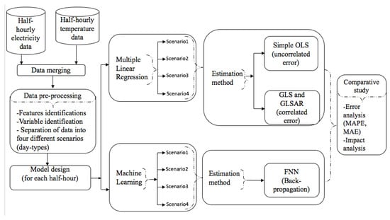
Figure 1.
Proposed forecasting methods.
After the detailed discussion of data characteristics and variable identification in Appendix A, and grouping methods of dataset in Section 1.2.3, the Thai dataset is carefully divided into four different subsets or hereafter named scenarios. Each model is trained and tested for each scenario and divided as,
- Scenario 1: only demand for working days.
- Scenario 2: only demand for weekends.
- Scenario 3: only holiday demand and highly fluctuated demand from December 24 to New Years eve.
- Scenario 4: all the demand dataset.
For each scenario, the parametric MLR model and non-parametric FF-ANN model were included in a comprehensive study.
2.1. Model Design
The variables are identified and presented in Appendix A.4 to construct the MLR and ANN models. The experiments show that an MLR forecasting model shows strong capability to build the relationship between model output and affecting variables. Similarly, ANN models have the strong capability of mapping the complex input/output relationship where we can construct a robust model for better results. These models are described as,
2.1.1. MLR Model Description
The electricity demand data is observed every half-hour, therefore there are observations in a day. Since we have total 84,618 observations, these datasets are made the half-hourly sectional grouping into 48 subsets. Each group contains the demand load for a specific hour of the day. Now, the individual subset is treated as a single series of data and all 48 series are modeled and estimated independently. Therefore, we have 48 individual forecasting models to forecast for one-day. The main advantage of implementing such a sectional form of data is that intra-day patterns are automatically avoided [17]. The demand at day d and half-hour for modeled as,
where , , and are groups of deterministic, temperature, historical electrical demand, and interaction terms, respectively. The residual modeling is very sensitive and important in MLR because of the incorporation of an auto-regressive structure in the error term. Such correlated errors assumed to follow an autoregressive with previous days. Therefore, Equation (2) describes that the current value of the error term at hour h of the day d is denoted by , which is the autoregressive sum of q previous days. We have run several models for different values of q. Mathematically,
The terms is the serially-correlated error term and . The Durbin–Watson (DW) test is used to test the hypothesis that the residuals are serially correlated or not. The hypothesis being tested as, for no serial correlation and for serially correlated error. The demand model can be written conveniently as a linear regression model,
Equation (3) consists of p predictor variables and the classification of these p variables are as in Equation (1), where . Depending on the properties of ∑, model is classified as,
- OLS: where errors
- GLS: for orbitrary covariance ∑
- GLSAR: where AR(p)
In our analysis, error terms are assumed to follow an AR(p) in days upto , therefore GLS turned as GLSAR methods, and implemented as,
Combining all 48 equations together in Equation (3), the half-hourly demand model can be written as,
Unlike simple regression context, , which is Seemingly Unrelated Regression (SUR) system describes that each row of corresponds to one day of half-hourly residuals is contemporaneously correlated but not correlated over a half-hour. This methodology is thoroughly explained in [17]. The auto-correlation AR(p), p=7 to the previous days was taken into account by taking lags, but not among the hours. The order of AR is determined by the significance test of ACF and PACF.
2.1.2. OLS and GLSAR Estimation
The MLR model designed in Equation (5) can be setup as, , for is the regression model for each half-hour h. Here, , , and . These regressors in the regression model are for half-hour h, and is the corresponding size matrix. This matrix contains the regressors from Equations (5). For instant, if , there exists 48 regressions, then where , , and is a . The serially correlated error (Equation (4)) term should be transformed to the serially uncorrelated error where , and i represents the number or order of the lag. Similarly, , and removes the serial correlation [19].
2.1.3. Performance Measurements
The most common criterion that is used for evaluation of forecasting performance is . It measures the deviation of forecasted value from a real value in terms of percentage.
where D represents the set of test days in the test dataset, and represents the real demand and predicted demand, respectively at day d and half-hour h.
2.2. Artificial Neural Network Approach
A neural network is a popular multi-stage powerful modeling tool that can capture the non-linear behavior and complex input to the output relationship compared to conventional techniques. The motivation for ANN construction is because of intelligent characteristics of neurons similar to the human brain because: a neural network acquired knowledge through learning, and this knowledge is stored as the weights within the inter-neuron connections. The mathematical expression for learning is,
The output function will be , where are the weights of each neurons; is a non-linear activation function.
2.2.1. Structure of ANNs
The structure of ANNs is composed of the numbers of layers and the neurons. The number of neurons is automatically fixed by the training data and the forecasting period. Moreover, the highlighted limitations associated with the ANN structure are that the training process oscillates and possible to converse at local minima. Some authors such as [24] discussed meta-heuristic methods to find the global minimum and selection of hidden neurons. Normally, the researcher gradually increases the number of neurons and compared them to the errors. Unlike shallow learning procedures, DNN refers to the combination of a large number of layers and neurons. Therefore, optimizing the depth and width of hidden layers is quite time consuming and not feasible to test all possible combinations. Therefore, we have determined the structure of DNN by the trial and error procedure and finally selected two hidden layers as discussed in Section 3.3 Table 5.
2.2.2. Activation Function
The activation function maps the resulting values by capturing the trends or feature patterns from the trained dataset. In ANN, the Rectified Linear Unit (ReLU) is considered as the excellent activation function to regularize the hidden layers. Since ReLU picks the , it avoids the vanishing gradient problem. Moreover, the advantage of ReLU is very quick to use and train the model so that computational cost is reduced compared to other activation functions. However, the learning process gets slow because of bias.
2.2.3. Resolving Overfitting
Over-fitting can be observed from the learning curve which describes the error rate according to the epochs. An epoch is just one cycle of iteration where the entire dataset is passed forward and backward in the network. Initially, a testing error is reduced by increasing the number of epochs in a trained model, but there exists a threshold point from where the testing error starts to increase even the training error seems improving. Therefore, over-fitting is a serious problem in ANN techniques which can be minimized by adding more observational data or using the concept of dropout. Dropout function randomly ignores or drops out some subset of nodes from a given layer during the training procedure so that it can prevent an over-fitting problem.
3. Results and Discussion
3.1. Selection of Training Length
To determine the best length of the training period, Scenario 1 was chosen due to less variation in the dataset. This dataset is implemented for OLS estimation considering the absence of serially correlated-error coefficients. The number of coefficients and size of the training dataset should not be over-parameterized. Scenario 1 consists of 54 coefficients and 236 to 911 set of observations obviously avoids the over-fitting problem [17]. Insufficient feature abstraction could happen in a short length of the training dataset. A longer length of training dataset provides more information to the forecasting model and obviously results in good accuracy. However, considering a longer training dataset, the forecasting accuracy can be affected if the historical pattern of data significantly differs from the most recent data [66]. Lusis et al. [66] suggested that just one-year length is sufficient for training to develop the residential electricity model. However, Clements et al. [21] implemented a three-year length of aggregate data for the Queensland region, Australia, where the model obtained quite impressive results with MAPE 1.36%. Since the length of the training dataset shows localized characteristics, four different sizes of training datasets, 911 days, 717 days, 475 days, and 236 days are tested. These four different sizes or cases are designed as,
- Case I: Training period: 911 days, test period: 239 days in the year 2013.
- Case II: Training period: 717 days, test period: 239 days in the year 2013.
- Case III: Training period: 475 days, test period: 239 days in the year 2013.
- Case IV: Training period: 236 days, test period: 239 days in the year 2013.
Forecasting accuracy and execution time were calculated for all four cases and tabulated in Table 1. When the training length is more than three years, both the methods: simple OLS, and FF-ANN forecast with the lowest MAPE. The Table 1 depicted the execution time (both training and testing) for MLR approach: simple OLS method is about 110 Sec for 239 days which is fairly good and acceptable. Therefore, more than three years of training length is picked up for further experiments in this paper.

Table 1.
Mean Absolute Percentage Error (MAPE) measures for different training lengths using the Scenario 1 dataset.
3.2. MLR Approach: Simple OLS Method
3.2.1. Model Selection
Normally, a perfect fit model can always be obtained by using a model with enough parameters and results in good training accuracy. However, better training accuracy does not guarantee better accuracy while forecasting with a testing dataset. Moreover, complexity is increased to analyze the interpretation of the model due to a large number of variables. Therefore, Table 2 presents the importance of some variables based on forecasting accuracy. The result reveals that the forecasting accuracy is improved by incorporating more independent variables. In this experiment, Senario 2 performs the best with MAPE of . This means the weekend demand forecasting model by the grouping of weekend data separately can forecast with the best accuracy for Saturday and Sunday. The Scenario 1 stands with competitive MAPE which is less than 2% because of holiday free working days, while Scenario 3, which consists of holidays forecast with the worst MAPE of . The model selection procedure for holiday is always challenging due to the significant variation of demand. The performance of Scenario 3 is the worst among others because of the most fluctuated dataset. Since Scenario 4 using all the dataset including holidays, can forecast with MAPE , we choose this Scenario 4 for holiday forecasting purpose.
Table 2.
Effect of variables on MAPE: simple Ordinary Least Square (OLS).
The continuous forecasting curves for Scenario 1 is presented Figure A8. The comparison of actual demand and prediction demand curves shows that most of the predictions are very closed to real demand. Since the forecasting is only for working days and non-holidays, only 239 days are predicted. Some predictions on the second week of December, the first weeks of January and April were found to have under-forecasted values because of the so-called holiday_effect affecting the bridge days of the holidays. Such occurrence of holidays adjacent to the working days forces to reduce the accuracy.
The columns of the Table 3 report R-squared, Adjusted R-squared, and DW values, respectively, for individual half-hours. R-squared and Adjusted R-squared are the goodness of fit measures.
Table 3.
Model description paramters: GLSAR-7 (Scenario 1).
Since these data are the results from the testing dataset, to of the variability in the testing dataset was accounted for by the predictor variable included in the model. Adjusted R-squared values are found normally lower than R-square indicating predictor variables improve the model. Adjusted R-squared increases only if the new term improves the model more than would be expected by chance. Similarly, the DW test is a statistical technique to determine whether the series follow auto-correlation or not. The residual for the individual half-hour was analyzed separately. DW statistic value is always between 0 and 4. Values less than 2 indicate positive auto-correlation and a value greater than 2 indicates negative autocorrelation. DW value equals 2 means there is no auto-correlation. Since most of the DW statistics for all 48 half-hours are found between to for simple OLS, there is some evidence to reject the null hypothesis. These statistics for simple OLS and GLSAR-7 are tabulated in Table 3 and compared DW values. The positively-correlated DW statistics (1.17–2.48) after 5 p.m. (HH) which was the evidence of serially correlated error, is now significantly improved nearly . This indicates that forecasting errors are now uncorrelated. The selection of a better statistical model from a set of candidate models is a crucial factor. Since the OLS results for Scenario 1 show MAPE which could still possibly to reduced by implementing AR lags on the model. To determine the number of AR lags, we have selected peak hour (2 p.m.) and tested for different lags such as 1 to 7 where p-values are found very small (less than 0.09), so we have strong evidence that the errors follow at least AR(7). Table 4 presents the MAPE for GLSAR(1) to GLSAR(7) indicating that GLSAR(7) got the lowest MAPE value.
Table 4.
MAPE measures for different model structures for Scenario 1.
3.2.2. Temperature Effect
The temperature-related variable and their effects on demand are expressed in Figure 2. This figure describes the rate of demand variation per degree temperature change from Monday to Saturday for individual months of a year 2013. While interpreting the demand variation for a particular day, Sunday is considered as the reference day. Similarly, Figure 2 presents such a variation for February to December where January is the reference month.
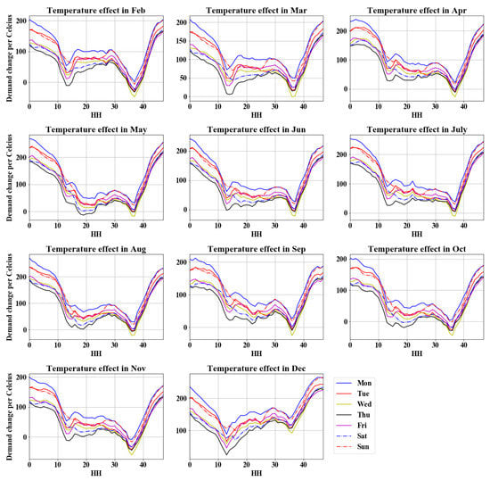
Figure 2.
Demand variation per degree change in temperature.
The rate of demand variation per degree temperature is minimum 50 MW/C approximately at morning hours 6 a.m.–7 a.m. and evening hours (5–6 p.m.) because most of the people during these hours are on the way to work or traveling back from work. The increment of 50 MW per 1 C is about of the average demand. Flat and consistent demand variation from 100 MW/C–200 MW/C which is 1.4–2.6% rise in demand throughout the day hours except on Saturday and Sunday. The graph line for Saturday and Sunday is significantly lower and different than other working days in the morning and office hours which is as our expectation. Since electricity demand reaches a peak during the day hours of summer in Thailand, our results surprisingly explain quite different scenarios. The highest demand variation per degree rise in temperature exists up to 300 MW/C which is rise per 1 C at 11 p.m. because most of the people are at home during this time. Such increment is lower than Greece [29], similar to the impact on aggregate demand of Singapore [38]. Since the temperature impact on residential demand is quite high [28,38], our result matches only to the impact of aggregate demand. The most interestingly, climate impact studied by Parkpoom et al. [8] also mentioned the similar result to our findings for the peak electricity demand of Thai data, however, the information about hours and days are lacking.
3.2.3. Special Day and AR Effect
The STDF models for special days such as Songkran, New Year and other special days are always challenging. The MAPE performance of these days is also poor in our study. However, the interpretation of coefficients is found realistic and expressed in Figure 3. The results present the different and distinct pattern groups. The demand variation after the holiday and after the long holiday significantly increased; while the demand reduced sharply for the special days. However, the working day after the special days increased as our expectations. If there is a regular holiday, demand on the next working day is increased because the people do not have time to travel far and come back to work quickly. However, on the next working day of other special events such as Songkran, and New Year, electricity demand significantly decreases because of the festive vibes on people. Many people during such festive holidays travel out of Bangkok to their hometown or travel plans and return to work a bit slow. Except for the day after the holiday and the flooding period, the electricity demand had a similar effect in the morning hours up to 5 a.m. and night hours after 8 p.m., while the demand was consistently at a high level on the day after a holiday. Similarly, demand was consistently at a lower level during the flooding period. The sudden and unexpected flooding period happened in Bangkok because of the shutdown of industries, commercial sectors, and universities. This situation is similar to the current Covid-19 and lockdown condition of Thailand.
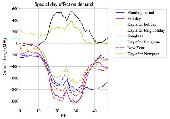
Figure 3.
Demand variation at individual half-hour for special days.
The contribution of AR error terms is plotted in Figure 4. AR1 represents the error terms of the same hour but one previous day, and AR2 represents the error terms of the same hour but two previous days. In this sequence, AR7 represents the error terms of the same hour but seven previous days which is ultimately the same weekday before a week. In our result, AR2–AR4 and AR6–AR7 show the normal correlation impact up to in the morning hours till 8 a.m. (HH). The maximum demand contribution is obtained from the one previous day which is up to while AR5 contributes to the lowest impact. The contribution pattern of AR1 is minimum early in the morning hours, while it increases gradually and reached a peak at 8 p.m. Since the demand profile of electricity is quite similar in the same hour of two consecutive days, it is obvious to have the maximum correlated error. As our expectation, AR7 contributes to the competitive impact on demand because of the same day and same hour of previous week i.e., similar day effect. A similar study for the lagged load correlations discussed in [17,21] also mentioned that the impact of AR1 has the highest contribution to the demand up to
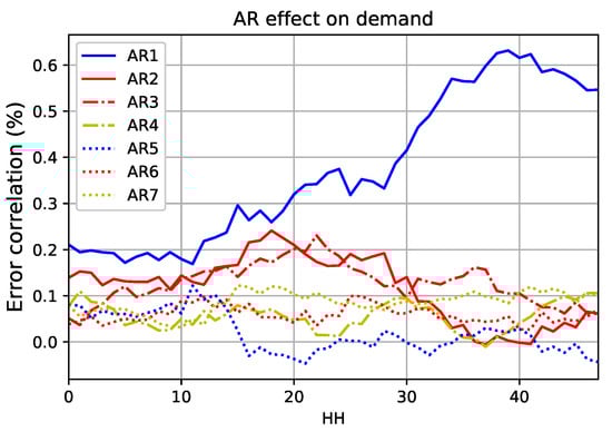
Figure 4.
Measure of correlated error for individual half-hour.
3.3. ANN Approach: FF-ANN: A Simple DNN
A simple FF-ANN is implemented to predict all the scenarios as defined before: Scenarios 1–4. Input variables were designed from patsy, a Python package already used for MLR methods. Since the non-linear relations between the variables are automatically captured by the DNN structure, initially we ignored the non-linear variables such as squared-temperature, and interactions of variables. However, later these terms were included in models due to improvement in accuracy.
Therefore, historical demand data with lag load1d_cut2pm, load7d, and Load2pmYesterday and their dependency terms on the temperature such as MaxTemp, MaxTempYesterday, MA2pmTemp are included in model. To avoid the over-fitting problem in DNN, selection of the best number of epochs, a number of hidden layers and nodes are very sensitive. An experiment was performed for various structures: 1, 2, 3, and 4 hidden layers with different nodes and few are tabulated in Table 5, explains that two hidden layer structures with nodes shows the best MAPE approx. 2.72% for testing data.
Table 5.
Selection of hidden layers, nodes and epochs for Scenario 1.
Unlike ARMAX methods, a trained FF-ANN model was used to forecast all the days of 2013. While in simple OLS, rolling windows of the training dataset are used to train for one step forward prediction. The reason behind this unfair methodology implied that FF-ANN took much longer to train a model compared to simple OLS or GLSAR. Therefore, the test period 2013 is divided into a small number of prediction intervals, named as pred_intervals. For example, if pred_intervals = 2, both training and testing dataset is divided into two halves. For the first half, we use the dataset from 8 March 2009 to 2012 as training to make predictions for January–June, 2013. For the second half, we used 08 March 2009 to June 2013 as training to make predictions from July–December, 2013 and so on. Moreover, the prediction was still one-day ahead where today’s demand data was used to predict tomorrow’s demand. The prediction error and computational time in Table 6 compared the performance of simple OLS and FF-ANN in terms of MAPE and execution time. The result shows that the forecasting accuracy of simple OLS is better for the same pred_intervals. When pred_intervals were increased, forecasting accuracy was improved for FF-ANN, but both execution time and MAPE performance are higher than simple OLS. This tradeoff concludes that simple OLS shows better performance than FF-ANN for our dataset. Since the FF-ANN method unable to compete with simple OLS and GLSAR, FF-ANN was therefore excluded for further comparison in Table 7. However, the MAPE of 2.56–2.89% obtained from FF-ANN was quite lower than some Thai-based published papers such as [22,23,50], where they implemented ANN-based methods for a half-hourly dataset.
Table 6.
Prediction error and computational time.
Table 7.
Forecasting accuracy (MAPE%) comparison: all scenarios.
A detailed comparison on performance in terms of forecasting accuracy shows that Scenario 1 from simple OLS predicted with lower MAPE compared to GLSAR for most of the working days except on Friday. The simple OLS can predict for Scenario 1 by MAPE value 1.81% which is quite impressive. However, forecasting accuracy for Friday, and working days after holidays are found better in GLSAR compared to simple OLS. The Scenario 3 did not perform well for holidays in either method, which concludes that grouping of holidays dataset can not forecast well. To predict holidays, Scenario 4 was better than Scenario 3 indicating that aggregate data grouping all datasets together provides a good result for holidays. However, the grouping of weekend datasets separately as Scenario 2 outperformed than simple OLS methods with MAPE value 1.74%. Darshana and Chawalit [24] implemented the hybrid PSO with GA for the same dataset again and improved the MAPE to which is still higher MAPE compared to this study.
3.4. Computation Time
A computational time in the forecast system was the length of execution time for a model. The main parameters of execution time are the length of training data, number of variables, processor speed of a computer, and forecasting methods. When the online forecast system is implemented for utility, real-time electricity demand observation data of each day automatically updated in the training dataset so that the execution time can increase. In our experimental setup three different forecasting methods were chosen by keeping other parameters constant. Although the computational time is not in the objective, the computation time of a model could be the crucial factor while choosing the best forecasting methods on similar performance. In this study, computational time to forecast for 24 h was approximately min for an OLS technique, whereas there was four times more computational time for GLSAR. If we follow a similar methodology, FF-ANN needs to forecast with Pre_intervals = 365 (Table 6) which may take several days, and we skipped it. These experiments were conducted on the system having the configuration, Intel Core i5 2.5 GHz processor with 8 GB of RAM.
3.5. Pro and Cons of the Methods
Under the consideration of linearity, homoscedasticity, and independent identically distributed data, the maximum likelihood solution to OLS is considered the best linear unbiased estimator. The implementation of OLS and its extension to GLSAR were the most efficient methods even for heteroscedasticity or auto-correlation to the interpretation of variables. The presence of non-linearity in the samples of a dataset can not be denied, therefore ANN is also implemented. However, these methods (OLS, GLSAR, and ANN) are sensitive to the outliers present in the dataset. Increasing the number of variables possibly causes over-fitting and increases the complexity of the interpretation of variables. For an unbiased estimate, we need the mean of the infinite beta parameter for an instance. In a real scenario, we have only one set of data for one instance. So, the possibility of ‘biased estimates’ cannot be denied. If we consider the quartile regression or Bayesian estimation, the possibility of unbiased estimation could be minimized.
4. Conclusions
This paper presents a novel approach for STDF by constructing four different scenarios so that the model can be trained with an appropriate training dataset. Selection of the proper variables for a model, length of the training dataset is conducted based on experiments. The performance on forecasting accuracy measured in terms of MAPE for Scenario 1 was obtained as 2.72%, , and for FF-ANN, GLSAR(7), and OLS, respectively. This means the proposed simple OLS and its extension to GLSAR methods outperformed the deep learning methodology on forecasting accuracy among four scenarios. Nevertheless, GLSAR had longer execution time than OLS, but significantly shorter than FF-ANN. Therefore, a further comparison of forecasting accuracy is conducted between simple OLS and its extension GLSAR methods. Normally, the atmosphere of Thailand is very hot during day hours and the general belief is that this hot temperature results in high demand for electricity during day hours. The minimum increment rate of demand approximately 50 MW per 1 C rise occurs at the morning hours (6 a.m.–7 a.m.) and evening hours (4 p.m.–6 p.m.). The low impact in the morning and evening is because of people at the no work condition as well as the industrial shift changing time. Throughout the day, the impact of temperature responsible for increases by 100 MW–200 MW per 1 C rise in temperature. However, the result reveals that the maximum impact of temperature is during night hours rather than day hours at 11 p.m. In this time most people are at home and there is excessive use of electric appliances such as television and other cooling appliances. The comparative study concluded that the forecasting error after the grouping of training dataset according to working days (), and weekends () provided better accuracy compared to the single group of training dataset Scenario 4 (), i.e., Scenario 1 gave a better forecasting accuracy for working days from simple OLS methods; Saturday and Sunday from Scenario 2. However, Scenario 3 showed the worst accuracy from both the models for holidays. Therefore, it is better to choose Scenario 4 (all the data together) rather than Scenario 3 (holidays data) to forecast the holidays.
Author Contributions
S.K. conceived and designed the models, wrote programs to clean up and visualize the data and conduct experiments, analyzed results, and drafted and revised the manuscript. K.C. conceived and designed the models, conducted the experiments, analyzed results, and drafted and revised the manuscript. P.K. conceived and designed the models and revised the manuscript. All authors have read and agreed to the published version of the manuscript.
Funding
The authors gratefully acknowledge the financial support provided by Thammasat University under the TU Research Scholar, Contract No. 2/22/2560.
Acknowledgments
We would like to express our sincere appreciation to EGAT and Assoc. Chawalit Jeenanunta, at SIIT for providing the necessary dataset used in this research. The authors are thankful to the editor and four anonymous reviewers for their constructive feedback, which improved the presentation and quality of the paper compared to the first submission.
Conflicts of Interest
The authors declare no conflicts of interest.
Abbreviations
The following abbreviations are frequently used in this manuscript:
| AC | Air Condition |
| AR | Auto-regression |
| ARMAX | Auto-regressive Moving Average with Exogenous Variable |
| CDD | Cooling Degree Day |
| Covid-19 | Corona Virus Disease 2019 |
| DW | Durbin–Watson |
| EGAT | Electricity Generating Authority of Thailand |
| FF-ANN | Feed Forward Artificial Neural Network |
| GA | Genetic Algorithm |
| GLSAR | Generalized Least Square Auto Regression |
| HWT | Holt Winters Triple |
| MAPE | Mean Absolute Percentage Error |
| MEA | Metropolitan Electricity Authority |
| MLR | Multiple linear regression |
| MW | Megawatt |
| OLS | Ordinary Least Square |
| PSO | Particle Swarm Optimization |
| STDF | Short-term Demand Forecasting |
| RegSARIMA | Regression Seasonal ARIMA |
| ReLU | Rectified Linear Unit |
| SVM | Support Vector Machine |
Appendix A. Data Pre-Processing
Figure Section
In this paper, half-hour aggregate demand data provided by EGAT from 1 March 2009 to 31 December 2013 are used. Out of 84,618 samples of observation, only eight half-hour samples on 10 March 2012 were missing. They filled a simple interpolation from nearby data [67]. The pattern of overall data over the year 2012 is presented in Figure A1. This figure depicts the demand for working days, weekends, and holidays (holiday in gray color). The demand for holidays are much lower than on other days and fluctuated in nature. Most of the case, such fluctuations of demand appears on January, April, May, and December.

Figure A1.
Complete demand profile for a year: 2012.
Our study area covers the metropolitan region (Bangkok and surrounding provinces: Bangkok, Pathum Thani, Nonthaburi, Nakhon Pathom, Samut Sakhon, and Samut Prakan) of Thailand. The electricity consumption of the metropolitan region alone is about of the total consumption in Thailand [8]. There are many factories, industrial parks, business offices and universities within these provinces. These sectors consume approximately 71% of the total consumption in the Bangkok metropolitan region where only 24% of demand arises from the residential sector [26]. Therefore, the demand for this region is dominated by industrial/commercial sectors. The pattern of MEA demand data exhibits a trend, seasonal patterns, weekly, daily, and holiday effects which are the nature of demand and are similar characteristics to many tropical countries [21,63].
Appendix A.1. Monthly and Seasonal Pattern
The hourly aggregate demand profile for 2012 is plotted in Figure A2a. To observe the stable variation of demand over time, a rolling window of 336 samples (samples of a week) is taken for the moving average. This plot indicates that the overall demand follows a linear trend and seasonality over time.

Figure A2.
(a) Hourly demand profile with seasonality and trend. (b) Monthly variation of demand. (c) Monthly variation of demand: 2010–2013.
Every year, the electricity demand increased from January to the maximum level in May, however the mean demand in April was lower due to the Songkran festival. The box plot in Figure A2b shows a level of demand for individual months, where each box represents the first quartile () and third quartile () with the median shown by the line in the box. The green spot near the median line represents the mean value. Among the months, December shows relatively lower demand than the rest. Every year, these monthly patterns of demand follow a similar level of demand except in 2011 (Figure A2c). Three month-long flooding during the last quarter of 2011 significantly reduces the demand.
Appendix A.2. Weekly, Daily and Holiday Patterns
A residential demand is volatile and challenging task to predict [13,37]. In our dataset, the residential demand is dominated by the demand of commercial sector produced by factories, offices, and industries so that the volatility of demand is reduced. Therefore, during Monday to Friday, the day hours demand at 2 p.m. reached to the peak (Figure A3a). During weekends and holidays, all the governmental and the private offices/factories are closed. This results the evening hours demand at 8 p.m. reached to peak due to dominant nature of residential sector. The working day, which falls on the next day of the holiday, demand of electricity is found at a lower level than normal working day as presented in Figure A3b. Therefore, this paper considers one important variable for DayAfterHoliday and included in models.

Figure A3.
(a) Intra-day variation of demand for working and special days. (b) Intra-day variation of demand on the working day (next day of holiday).
In Figure A4a–c, a long holiday, New Year, and an Songkran festival, respectively, significantly pulls down the demand. These events normally falls in the first week of January (long holiday and New Year holiday, Figure A4a,b), the second week of April (Songkarn holiday, Figure A4c), respectively. During these periods, factories, universities, and other offices are closed for a week. During long holidays/religious holidays (Songkran festival), most of the people travel outside the metropolitan region. Therefore, there is low demand during a holiday or such a special event. Other holidays such as Mother’s Day (August 12) and Father’s Day (December 5) also affect demand, which is not as significant compared to Songkran and New Year. These effects on electricity demand are so-called holiday effect and plays an important role while modeling. Even in working days near to these holidays, demand is highly volatile e.g., the first week and last week of December; which is the main challenge to the researcher. These mentioned events falls on a fixed calender. There are some other festivals which fall on varied date such as Makha Bucha, Visakha Bucha and also locally celebrated other holidays exist in Thailand. Therefore, forecasting the demand for holidays, special events, and analyzing the impact during these days is quite challenging because the researcher need to add the complexity on the model with many variables.
The massive flooding in Thailand, popular known as Bangkok flood caused a significant demand drop from the October 2011 until the January 2012. Many factories, universities, offices in Bangkok and surrounding provinces were locked down for entire periods. Figure A4d compares the level of demand drop on flooding duration with respect to the same date of previous year. During that the peak demand was reduced approximately by 2000 MW. In this paper, we have discussed the impact of such a unexpected flooding to the electricity demand.

Figure A4.
(a) Impact of long holiday on electricity demand. (b) Impact of New Year on electricity demand. (c) Impact of Sonkran festival on electricity demand (d) Impact of massive Bangkok flood on electricity demand.
Appendix A.3. Temperature
The effect of climate variables, especially the temperature is widely studied and included in STDF models [19,20,22,23,24,25,50,68]. The geographical variability shows strong impacts on heating effect in cold countries, whereas a strong cooling effect in warm countries [19]. Thailand is a tropical country having an approximate mean temperature which ranges from 25 C in December to 30 C in May. People face a warm atmosphere and feel very hot during summer. Therefore, the use of cooling devices occurs on a large scale in Thailand. Moreover, the economic status of the country is also rising, which supports the use of cooling devices such as air-conditioners. Regardless, geographic variability and economic activities are excluded from this study. Figure A5a explains the variation of demand due to temperature for holiday and non-holiday at peak hours (2 p.m.). Unlike the many articles [19,41], electricity demand is sharp and linear during working days. There is no significant variation in peak demand due to temperature. This fact supports the article [11,13] that commercial demand does not much vary with temperature. When temperature level drops down from 30 C or increase from 35 C high variation of demand on a holiday takes place. Since we are dealing with a separate model for individual hours, characteristics of demand at two different hours are presented in Figure A5b. This figure compares the relationship between temperature and peak demand at 2 p.m. and 11 p.m. Figure A5b indicates that on working days, the night hour at 11 p.m. shows a more linear relationship to the demand compared to the demand at 2 p.m., indicating that the impact of temperature should be more during night 11 p.m.

Figure A5.
(a) Effect of temperature during peak hour. (b) Effect of temperature at two different hours.
In general, most of the papers [19,38,41,68] describe a non-linear relationship between electricity demand and temperature. Figure A6 presents the relationship between temperature and electricity demand at for all the days of a week. The representation of the days is considered as Weekday = 0 means Monday, Weekday = 1 means Tuesday and so on. For each day, this Figure A6 shows the linear relationship thoroughly over a weekday as the proof for the positive linear impact of temperature for Thai demand. Such a linear relationship of electricity demand with respect to temperature is due to the dominant nature of industrial demand of the Bangkok region. This implies that we can exclude the non-linear terms of temperature. Nevertheless, our experiment shows that forecasting accuracy is improved by including non-linear terms of temperature. That means some non-linear relationship cannot be excluded during other hours of the day. Therefore, we have included a non-linear variable in our models to increase forecasting accuracy.

Figure A6.
Effect of temperature for electricity demand on working day at peak hour: 2 p.m.
Appendix A.4. Variable Identification
Many authors such as [69,70] proposed and implemented a cross-validation strategy for the variable selection strategy in their forecasting model. In our study, various aspects of data analysis are observed in an Appendix A such as seasonal patterns, holiday, weekly, and daily patterns. External variables such as weather variables (in our case: temperature) and their interactions with days and months have been explicitly included in our forecasting models.

Figure A7.
Demand prediction horizon: practice in Thailand.
Ramanathan et al. [17] suggested to implement the dummy variables and their interactions. They have considered the Sunday as a public holiday because the demand level of Sunday is quite similar to the demand for a holiday. Cottet et al. [51] applied five different day-type dummy variables to the days of a week. Considering these facts, this paper grouped the variables into four different categories as, deterministic, temperature, lagged, interactions and tabulated in Table A1. For simplicity lagged terms and prediction horizon for Thailand practice are presented in Figure A7. This study follows a similar strategy. To forecast for the demand on day ‘d’, one day ahead demand (previous day) dataset means the demand data of to of day and to of day represented by same variable load1d_cut2pm. Similarly, two days ahead lagged demand also implemented in our model represented by variable load2d_cut2pm. The terms load3d_cut2pmR and load4d_cut2pmR are also implemented by EGAT to make a forecast for Sunday and Monday from Friday 2 p.m. which is excluded form this paper.
Table A1.
List of selected input variables.
Table A1.
List of selected input variables.
| Types | Variables | Description |
|---|---|---|
| Deterministic | WD | Week dummy [Mon <Tue ...<Sat<Sun] |
| MD | Month dummy [Feb <Mar <...<Nov <Dec] | |
| DayAfterHoliday | Binary 0 or 1 | |
| DayAfterLongHoliday | Binary 0 or 1 | |
| DayAfterSongkran | Binary 0 or 1 | |
| DayAfterNewyear | Binary 0 or 1 | |
| Temperature | Temp | Forecasted temperature |
| MaxTemp | Maximum forecasted temperature | |
| Square temperature | Square of the forecasted temperature | |
| MA2pmTemp | Moving avearage of temperature at 2pm | |
| Lagged | load1d_cut2pm | 1 day ahead untill 2pm and 2 day ahead after 2pm load |
| load2d_cut2pm | 2 days ahead untill 2pm and 3 day ahead after 2pm load | |
| load3d_cut2pmR | 3 days ahead untill 2pm and 4 days ahead after 2pm load | |
| load4d_cut2pmR | 4 days ahead untill 2pm and 5 days ahead after 2pm load | |
| Interaction | WD:Temp | Interaction of week day dummy to temperature |
| MD:Temp | Interaction of month dummy to temperature | |
| WD:load1d_cut2pm | Interaction of week day dummy to load1d_cut2pm | |
| WD:load2d_cut2pm | Interaction of week day dummy to load2d_cut2pm |
Appendix B. Figures and Tables
Figure Section

Figure A8.
Forecasting performance of OLS (Scenario 1).

Figure A9.
Forecasting performance of OLS (Scenario 4).

Figure A10.
Forecasting performance of OLS for September 2013 (Scenario 4).

Figure A11.
(a) Forecasting during Sonkran festival (Scenario 4). (b) Forecasting during last week of December (Scenario 4).
References
- Murakoshi, C.; Namagami, H.; Xuan, J.; Takayama, A.; Takayama, H. State of residential energy consumption in Southest Asia: Need to promote smart appliances because urban household consumption is higher than some develped countries. ECEEE Summer Study Proc. 2017, 1489–1499. Available online: https://www.eceee.org/library/conference_proceedings/eceee_Summer_Studies/2017/7-appliances-products-lighting-and-ict/state-of-residential-energy-consumption-in-southeast-asia-need-to-promote-smart-appliances-because-urban-household-consumption-is-higher-than-some-developed-countries/ (accessed on 4 May 2020).
- Panklib, K.; Prakasvudhisarn, C.; Khummongkol, D. Electricity Consumption Forecasting in Thailand Using an Artificial Neural Network and Multiple Linear Regression. Energy Sources Part B Econ. Plan. Policy 2015, 10, 427–434. [Google Scholar] [CrossRef]
- ADB. Key Indicators for Asia and the Pacific 2017. Online 2017. Available online: https://www.adb.org/sites/default/files/publication/357006/06-rt-energy-electricity.pdf (accessed on 1 May 2020).
- Kaur, N.; Sood, S.K. An Energy-Efficient Architecture for the Internet of Things (IoT). IEEE Syst. J. 2017, 11, 796–805. [Google Scholar] [CrossRef]
- Samson, O. Electricity and the Fourth Industrial Revolution. 2018. Available online: https://www.researchgate.net/publication/324876698_ELECTRICITY_AND_THE_FOURTH_INDUSTRIAL_REVOLUTION (accessed on 4 May 2020).
- Clarke, L.; Jiang, K.; Akimoto, K.; Babiker, M.; Blanford, G.; Fisher-Vanden, K.; Hourcade, J.C.; Krey, V.; Kriegler, E.; Löschel, A.; et al. Chapter 6—Assessing transformation pathways. In Climate Change 2014: Mitigation of Climate Change. IPCC Working Group III Contribution to AR5; Cambridge University Press: Cambridge, UK, 2014. [Google Scholar]
- Momami, M. Factors Affecting Electricity Demand in Jordan. Energy Power Eng. 2013, 5, 50–58. [Google Scholar] [CrossRef]
- Parkpoom, S.; Harrison, G.P. Analyzing the Impact of Climate Change on Future Electricity Demand in Thailand. IEEE Trans. Power Syst. 2008, 23, 1441–1448. [Google Scholar] [CrossRef]
- Mideksa, T.; Kallbekken, S. The impact of climate change on the electricity market: A review. Energy Policy 2010, 38, 3579–3585. [Google Scholar] [CrossRef]
- McCulloch, J.; Ignatieva, K. Forecasting High Frequency Intra-Day Electricity Demand Using Temperature. SSRN Electr. J. 2017. [Google Scholar] [CrossRef]
- Julian, M.C.; Julian, P. Temperature effects on firms’ electricity demand: An analysis of sectorial differences in Spain. Appl. Energy 2015. [Google Scholar] [CrossRef]
- Hossein Motlagh, N.; Mohammadrezaei, M.; Hunt, J.; Zakeri, B. Internet of Things (IoT) and the Energy Sector. Energies 2020, 13. [Google Scholar] [CrossRef]
- Csoknyai, T.; Legardeur, J.; Akle, A.A.; Horvath, M. Analysis of energy consumption profiles in residential buildings and impact assessment of a serious game on occupants behavior. Energy Build. 2019, 196, 1–20. [Google Scholar] [CrossRef]
- Serralles, R.J. Electric energy restructuring in the European Union: Integration, subsidiarity and the challenge of harmonization. Energy Policy 2006, 34, 2542–2551. [Google Scholar] [CrossRef]
- Chapagain, K.; Kittipiyakul, S. Short-Term Electricity Demand Forecasting with Seasonal and Interactions of Variables for Thailand. In Proceedings of the 2018 Int Electrl Eng Congress (iEECON), Krabi, Thailand, 7–9 March 2018; pp. 1–4. [Google Scholar] [CrossRef]
- Taylor, J.W.; de Menezes, L.M.; McSharry, P.E. A comparison of univariate methods for forecasting electricity demand up to a day ahead. Int. J. Forecast. 2006, 22, 1–16. [Google Scholar] [CrossRef]
- Ramanathan, R.; Engle, R.; Granger, C.W.; Vahid-Araghi, F.; Brace, C. Short-run forecasts of electricity loads and peaks. Int. J. Forecast. 1997, 13, 161–174. [Google Scholar] [CrossRef]
- Dordonnat, V.; Koopman, S.J.; Ooms, M. Dynamic factors in periodic time-varying regressions with an application to hourly electricity load modelling. Comput. Stat. Data Anal. 2012, 56, 3134–3152. [Google Scholar] [CrossRef]
- Chapagain, K.; Kittipiyakul, S. Performance Analysis of Short-Term Electricity Demand with Atmospheric Variables. Energies 2018, 11, 818. [Google Scholar] [CrossRef]
- Chapagain, K.; Kittipiyakul, S. Short-term Electricity Load Forecasting Model and Bayesian Estimation for Thailand Data. In Proceedings of the 2016 Asia Conf on Power and Electl Engg (ACPEE 2016), Bankok, Thailand, 20–22 March 2016; Volume 55, p. 06003. [Google Scholar]
- Clements, A.E.; Hurn, A.S.; Li, Z. Forecasting day-ahead electricity load using a multiple equation time series approach. Eur. J. Oper. Res. 2016, 251, 522–530. [Google Scholar] [CrossRef]
- Phyo, P.; Jeenanunta, C. Electricity Load Forecasting using a Deep Neural Network. Eng. Appl. Sci. Res. 2019, 46, 10–17. [Google Scholar]
- Su, W.H.; Jeenanunta, C. Short-term Electricity Load Forecasting in Thailand: An Analysis on Different Input Variables. In IOP Conference Series: Earth and Environmental Science; IOP Publishing: Bristol, UK, 2018. [Google Scholar] [CrossRef]
- Darshana, A.K.; Chawalit, J. Hybrid Particle Swarm Optimization with Genetic Algorithm to Train Artificial Neural Networks for Short-term Load Forecasting. Int. J. Swarm Intell. Res. 2019, 10, 1–14. [Google Scholar]
- Chapagain, K.; Sato, T.; Kittipiyakul, S. Performance analysis of short-term electricity demand with meteorological parameters. In Proceedings of the 2017 14th Int Conf on Electl Eng/Elx, Computer, Telecom and IT (ECTI-CON), Phuket, Thailand, 27–30 June 2017; pp. 330–333. [Google Scholar]
- Ministry, E. Energy data visualaization for Thailand. Energy Policy Plan. Off. 2020. Available online: http://www.eppo.go.th/index.php/en/ (accessed on 2 May 2020).
- Wangpattarapong, K.; Maneewan, S.; Ketjoy, N.; Rakwichian, W. The impacts of climatic and economic factors on residential electricity consumption of Bangkok Metropolis. Energy Build. 2008, 40, 1419–1425. [Google Scholar] [CrossRef]
- Cian, D.E.; Lanzi, E.; Roberto, R. The Impacts of Temperature Change on Energy Demand: A Dynamic Panel Analysis. SSRN Electr. J. 2007. [Google Scholar] [CrossRef]
- Mirasgedis, S.; Sarafidis, Y.; Georgopoulou, E.; Kotroni, V.; Lagouvardos, K.; Lalas, D. Modeling framework for estimating impacts of climate change on electricity demand at regional level: Case of Greece. Energy Convers. Manag. 2007, 48, 1737–1750. [Google Scholar] [CrossRef]
- Masood, N.A.; Sadi, M.Z.; Deeba, S.R.; Siddique, R.H. Temperature Sensitivity Forecasting of Electrical Load. In Proceedings of the 2010 4th International Power Engineering and Optimization Conference (PEOCO), Shah Alam, Malaysia, 23–24 June 2010. [Google Scholar]
- Istiaque, A.; Khan, S.I. Impact of Ambient Temperature on Electricity Demand of Dhaka City of Bangladesh. Sci. Res. Publ. 2018, 10, 319–331. [Google Scholar] [CrossRef]
- Zhang, C.; Liao, H.; Mi, Z. Climate impacts: Temperature and electricity consumption. Nat. Hazards 2019, 99, 1259–1275. [Google Scholar] [CrossRef]
- Zhang, M.; Zhang, K.; Hu, W.; Zhu, B.; Wang, P.; Wei, Y.M. Exploring the climatic impacts on residential electricity consumption in Jiangsu, China. Energy Policy 2020, 140, 111398. [Google Scholar] [CrossRef]
- Li, B.; Lu, M.; Zhang, Y.; Huang, J. A Weekend Load Forecasting Model Based on Semi-Parametric Regression Analysis Considering Weather and Load Interaction. Energies 2019, 12, 3820. [Google Scholar] [CrossRef]
- Bessec, M.; Fouquau, J. The non-linear link between electricity consumption and temperature in Europe: A threshold panel approach. Energy Econ. 2008, 30, 2705–2721. [Google Scholar] [CrossRef]
- Asadoorian, M.O.; Eckaus, R.S.; Schlosser, C.A. Modeling climate feedbacks to electricity demand: The case of China. Energy Econ. 2008, 30, 1577–1602. [Google Scholar] [CrossRef]
- Chang, Y.; Kim, C.S.; Miller, J.I.; Park, J.Y.; Park, S. A new approach to modeling the effects of temperature fluctuations on monthly electricity demand. Energy Econ. 2016, 60, 206–216. [Google Scholar] [CrossRef]
- Ang, B.; Wang, H.; Ma, X. Climatic influence on electricity consumption: The case of Singapore and Hong Kong. Energy 2017, 127, 534–543. [Google Scholar] [CrossRef]
- Fung, W.; Lam, K.; Hung, W.; Pang, S.; Lee, Y. Impact of urban temperature on energy consumption of Hong Kong. Energy 2006, 31, 2623–2637. [Google Scholar] [CrossRef]
- Maheshwari, A.; Murari, K.K.; Jayaraman, T. Peak Electricity Demand and Global Warming in the Industrial and Residential areas of Pune: An Extreme Value Approach. arXiv 2019, arXiv:1908.08570. [Google Scholar]
- Li, Y.; Pizer, W.A.; Wu, L. Climate change and residential electricity consumption in the Yangtze River Delta, China. Proc. Natl. Acad. Sci. USA 2019, 116, 472–477. [Google Scholar] [CrossRef] [PubMed]
- Apadula, F.; Bassini, A.; Elli, A.; Scapin, S. Relationships between meteorological variables and monthly electricity demand. Appl. Energy 2012, 98, 346–356. [Google Scholar] [CrossRef]
- Sailor, D.; Pavlova, A. Air conditioning market saturation and long-term response of residential cooling energy demand to climate change. Energy 2003, 28, 941–951. [Google Scholar] [CrossRef]
- Lopez, M.; Sans, C.; Valero, S.; Senabre, C. Classification of Special Days in Short-Term Load Forecasting: The Spanish Case Study. Energies 2019, 12, 1253. [Google Scholar] [CrossRef]
- Darbellay, G.A.; Slama, M. Forecasting the short-term demand for electricity: Do neural networks stand a better chance? Int. J. Forecast. 2000, 16, 71–83. [Google Scholar] [CrossRef]
- Hippert, H.; Bunn, D.; Souza, R. Large neural networks for electricity load forecasting: Are they overfitted? Int. J. Forecast. 2005, 21, 425–434. [Google Scholar] [CrossRef]
- Chapagain, K.; Kittipiyakul, S. Short-term Electricity Load Forecasting for Thailand. In Proceedings of the 2018 15th International Conference on Electrical Engineering/Electronics, Computer, Telecommunications and Information Technology (ECTI-CON), Chiang Rai, Thailand, 18–21 July 2018; pp. 521–524. [Google Scholar] [CrossRef]
- Srinivasan, D.; Chang, C.S.; Liew, A.C. Demand forecasting using fuzzy neural computation, with special emphasis on weekend and public holiday forecasting. IEEE Trans. Power Syst. 1995, 10, 1897–1903. [Google Scholar] [CrossRef]
- Ziel, F. Modeling Public Holidays in Load Forecasting: A German Case Study. J. Mod. Power Syst. Clean Energy 2018, 6, 191–207. [Google Scholar] [CrossRef]
- Darshana, A.K.; Chawalit, J. Combine Particle Swarm Optimization with Artificial Neural Networks for Short-Term Load Forecasting. Int. Sci. J. Eng. Technol 2017, 1, 25–30. [Google Scholar]
- Cottet, R.; Smith, M. Bayesian Modeling and Forecasting of Intraday Electricity Load. J. Am. Stat. Assoc. 2003, 98, 839–849. [Google Scholar] [CrossRef]
- Soares, L.J.; Medeiros, M.C. Modeling and forecasting short-term electricity load: A comparison of methods with an application to Brazilian data. Int. J. Forecast. 2008, 24, 630–644. [Google Scholar] [CrossRef]
- Papalexopoulos, A.D.; Hesterberg, T.C. A regression-based approach to short-term system load forecasting. IEEE Trans. Power Syst. 1990, 5, 1535–1547. [Google Scholar] [CrossRef]
- Ismail, Z.; Jamaluddin, F.; Jamaludin, F. Time Series Regression Model for Forecasting Malaysian Electricity Load Demand. Asian J. Math. Stat. 2008, 1, 139–149. [Google Scholar] [CrossRef]
- Dilhani, M.H.M.R.S.; Jeenanunta, C. Daily electric load forecasting: Case of Thailand. In Proceedings of the 2016 7th Int Conf of Inf and Comm Tech for Embedded Sys (IC-ICTES), Bangkok, Thailand, 20–22 March 2016; pp. 25–29. [Google Scholar] [CrossRef]
- Hippert, H.S.; Pedreira, C.E.; Souza, R.C. Neural networks for short-term load forecasting: A review and evaluation. IEEE Trans. Power Syst. 2001, 16, 44–55. [Google Scholar] [CrossRef]
- Hong, T.; Wang, P. Fuzzy interaction regression for short term load forecasting. Fuzzy Opt. Decis. Mak. 2014, 13, 91–103. [Google Scholar] [CrossRef]
- Shi, H.; Xu, M.; Li, R. Deep Learning for Household Load Forecasting Novel Pooling Deep RNN. IEEE Trans. Smart Grid 2018, 9, 5271–5280. [Google Scholar] [CrossRef]
- Asaleye, D.A.; Breen, M.; Murphy, M.D. A Decision Support Tool for Building Integrated Renewable Energy Microgrids Connected to a Smart Grid. Energies 2017, 10, 1765. [Google Scholar] [CrossRef]
- Sigauke, C.; Chikobvu, D. Peak electricity demand forecasting using time series regression models: An application to South African data. J. Stat. Manag. Syst. 2016, 19, 567–586. [Google Scholar] [CrossRef]
- Sigauke, C. Regression-SARIMA modelling of daily peak electricity demand in South Africa. J. Energy South. Afr. 2012, 23, 23–30. [Google Scholar]
- Haben, S.; Giasemidis, G.; Ziel, F.; Arora, S. Short term load forecasting and the effect of temperature at the low voltage level. Int. J. Forecast. 2019, 35, 1469–1484. [Google Scholar] [CrossRef]
- Soares, L.J.; Souza, L.R. Forecasting electricity demand using generalized long memory. Int. J. Forecast. 2006, 22, 17–28. [Google Scholar] [CrossRef]
- Sigauke, C.; Nemukula, M.M.; Maposa, D. Probabilistic Hourly Load Forecasting Using Additive Quantile Regression Models. Energies 2018, 11, 2208. [Google Scholar] [CrossRef]
- Botoc, C.; Anton, S.G. Is Profitability Driven by Working Capital Management? Evidence for High-growth Firms from Emerging Europe. J. Bus. Econ. Manag. 2017, 18, 1135–1155. [Google Scholar] [CrossRef]
- Lusis, P.; Khalilpour, K.; Andrew, L.; Liebman, A. Short-term residential load forecasting: Impact of calendar effects and forecast granularity. Appl. Energy 2017, 205, 654–669. [Google Scholar] [CrossRef]
- Goodwin, R. Convert Irregular Time Sereis to Hourly Data in Python and Have Normal Distribution. 2018. Available online: https://stackoverflow.com/questions/51392012/convert-irregular-time-series-to-hourly-data-in-python (accessed on 10 April 2020).
- Hor, C.; Watson, S.J.; Majithia, S. Analyzing the impact of weather variables on monthly electricity demand. IEEE Trans. Power Syst. 2005, 20, 2078–2085. [Google Scholar] [CrossRef]
- Hong, T.; Wang, P.; Willis, H.L. Short Term Electric Load Forecasting. Int. J. Forecast. 2010, 74, 1–6. [Google Scholar] [CrossRef]
- Wang, Y.; Niu, D.; Ji, L. Short-term power load forecasting based on IVL-BP neural network technology. Syst. Eng. Procedia 2012, 4, 168–174. [Google Scholar] [CrossRef]
© 2020 by the authors. Licensee MDPI, Basel, Switzerland. This article is an open access article distributed under the terms and conditions of the Creative Commons Attribution (CC BY) license (http://creativecommons.org/licenses/by/4.0/).