Abstract
The crankshaft dynamics model is of vital importance to a multitude of aspects on engine diagnostics; however, systematic investigations of such models performance (especially for large two-stroke diesel engines that are widely used in the power generation and shipping industries) have not been reported in the literature. This study aims to cover this gap by systematically investigating the parameters that affect the performance of a two-stroke diesel engine crankshaft dynamics model, such as the numerical scheme as well as the engine components inertia and friction. Specifically, the following alternatives are analysed: (a) two optimal performing numerical schemes, in particular, a stiff ordinary differential equations (ODE) solver and a fast solver based on a piecewise Linear Time-Invariant (LTI) scheme method, (b) the linear and the non-linear inertia-speed approaches, and (c) three engine friction submodels of varying complexity. All the potential combinations of the alternatives are investigated, and the crankshaft dynamics model performance is evaluated by employing Key Performance Indicators (KPIs), which consider the results accuracy compared to the measured data, the computational time, and the energy balance error. The results demonstrate that the best performing combination includes the stiff ODE solver, the constant inertia-speed approach and the most simplistic engine friction submodel. However, the LTI numerical scheme is recommended for applications that require fast response due to the significant savings in computational time with an acceptable compromise in the model results accuracy.
1. Introduction
Large two-stroke engines remain amongst the most efficient commercially available internal combustion engines, and are extensively used in shipping and power generation applications [1,2]. However, by considering the existing and future stringent environmental regulations targets as well as the need for reducing the operating cost and increasing efficiency [3,4], improving the insight and understanding of both the thermo-chemical phenomena and the dynamic response of these engines is of vital importance [5,6]. Specifically, thermodynamic models are extensively used for representing the engine thermo-chemical processes [7,8,9], whereas crankshaft dynamics models [10,11,12] are widely employed for simulating the engine drivetrain dynamics.
Crankshaft dynamics models are extensively used in a wide spectrum of internal combustion engines applications, which can be categorised as distributed mass or lumped mass models. The former employs the finite element method with the detailed crankshaft geometry, and is used primarily for crankshaft design applications, such as dynamic stress analysis [13,14,15], vibration analysis [16,17,18], and structural optimisation [19,20]. The latter approximates the crankshaft mass distribution using discrete masses corresponding to the engine cylinders, damper(s), chain drives, flywheel, shafting system, and engine load. Most importantly, as the engine crankshaft along with the connected shafting system is a non-linear flexible body, this model provides a relationship between the in-cylinder processes (characterised by the in-cylinder pressure) and the Instantaneous Crankshaft Speed (ICS), the Instantaneous Crankshaft Torque (ICT), and the crankshaft angular deformation, at a relatively low computational cost [21,22]. In this respect, lumped mass models combined with readily measured engine parameters, such as the ICS and the ICT, can be used to provide useful information for the engine processes control [23,24,25,26] and diagnostics [27]. In particular, fluctuations of ICS were utilised for misfire detection [12] and coupled with an artificial neural network to detect the fuel pump leakage [28]. Furthermore, the ICT is employed for diagnostic purposes, such as determination of the peak pressure position [25], reconstruction of the in-cylinder pressure diagram [29,30,31], and determination of the cylinder imbalances due to combustion [32,33].
Hence, due to its importance, efforts in the literature have been dedicated to the prediction of the engine ICT. Specifically, the most simplistic methods predict the ICT by employing a two-inertia lumped mass model [34,35,36], with significant efforts focused on the engine components friction prediction [37]. For multi-cylinder automotive engines, the ICT was adequately predicted by employing the variable inertia-speed approach [11], which provides the most complex form of the governing equations in the lumped mass model [38]. For the same engine type, reducing the computational time is realised by using a less complex model, which employs a constant inertia-speed approach according to which, the reciprocating pistons variable inertia and the engine shaft instantaneous rotational speed were assumed as constant [11,39]. For heavy duty diesel engines, the engine crankshaft dynamics model was used in its full complexity considering a variable inertia-speed approach [40] along with more sophisticated engine friction submodels [41]. In a recent study [10], a lumped mass model for a two-stroke diesel generator set was employed to predict ICT combines with Fourier series expansion and an iterative optimisation scheme for improving the model prediction accuracy.
From the pertinent literature review, it is inferred that there has not been a systematic consideration of different factors that affect the performance of the lumped mass model in regards to ICT prediction, especially considering large two-stroke engines. Specifically, the following three main gaps have been identified in the literature:
- The numerical schemes employed to solve the complicated systems of non-linear ordinary differential equations, which are essential to the crankshaft dynamics model performance, have been discussed only in few studies and are not analysed in detail [10,11].
- The benefits in the implementation of the constant inertia-speed approach, which significantly simplifies the crankshaft dynamics model, have not been investigated for engines with significantly larger rotating and reciprocating masses such as the large two-stroke engines.
- The effect of engine friction consideration on the ICT prediction still remains uncertain, as in some cases, complex submodels were employed [27,37,41], whereas more simplistic submodels are considered in other studies [23,40].
In this respect, this study aims to systematically investigate the performance of a two-stroke diesel engine crankshaft dynamics model as well as to benchmark alternative levels of model complexity, based on specific Key Performance Indicators (KPIs). This is performed by considering various numerical schemes, inertia-speed approaches, and engine friction submodels as listed below in order to investigate the following alternatives: (a) the two most prominent numerical schemes for solving the system of differential equations, (b) the variable and the constant inertia-speed approaches, and (c) three engine friction submodels of varying complexity (from simpler to most complex). The novelty of this study stems from the in depth and systematic investigation of the various combinations on setting up a crankshaft dynamics model for a large two stroke engine, thus providing a better understanding of the underlying parameters that affect the model’s predictive accuracy and simulation time as well as their interconnections, thus guiding the future developments of these engines dynamics modelling.
2. Materials and Methods
The methodology employed in this study consists of the following eight steps:
- Reference system selection: The reference system of a large two-stroke engine is selected for this investigation, and its operational and geometrical characteristics are described.
- Crankshaft dynamics model development: The model governing equations are derived considering both the variable and constant inertia-speed approaches for the reference system.
- Engine friction submodels: Three friction submodels are described and their integration into the model governing equations (Step 2) is explained.
- Numerical schemes: The implementation of the two most prominent numerical schemes for solving the set of differential equations of the reference system’s crankshaft dynamics model are described.
- Time step study: A time step study for the numerical schemes is performed where applicable, and the recommended time step is identified by using the convergence criterion and computational time.
- Identification of the KPIs to be used for the systematic comparison of the considered model alternatives.
- Systematic comparison of the investigated alternatives: The model results of all the possible combinations are compared based on the KPIs developed in step 6.
- Recommendations: The recommendations are discussed for the setup and usage of large two-stroke engines’ crankshaft dynamics models.
2.1. Reference System
The reference system considered in this study is a large two-stroke diesel engine driving an electric generator operating at a constant rotational speed of 124 r/min. The engine consists of 10 cylinders connected in an in-line configuration and has a Maximum Continuous Rating (MCR) of MW. The engine shafting system (engine crankshaft, coupling and generator shaft) is modelled by considering 16 Degrees Of Freedom (DOFs), with the first one corresponding to the torsional vibration damper and the last one corresponding to the electric generator. The engine also includes a chain drive between cylinders 5 and 6, which is also considered as a separate DOF. The reference system components as well as the considered DOFs are depicted in the schematic shown in Figure 1. The technical characteristics of the reference system were obtained from [10,27] and are discussed in detail in Section 2.7.
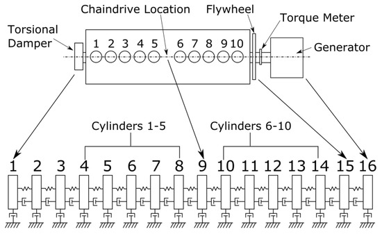
Figure 1.
Reference system schematic and equivalent lumped mass model.
2.2. Crankshaft Dynamics Model
The crankshaft dynamics of the reference system is modelled using a lumped mass model approach, the governing equations of which are derived by considering the shafting system’s torque balance by also taking into account the shafting system’s torsional flexibility. Specifically, the sum of the reciprocating and rotating masses torque , the structural damping torque , and the stiffness torque , must be equivalent to the sum of the combustion gases torque , the load torque , and the engine friction torque acting on each DOF as shown in Equation (1).
Presented in its rigorous format, Equation (1) forms a system of ordinary differential equations as represented by Equation (2) [11].
where symbols in bold represent vectors or vectored valued functions of the angular displacement vectors and its derivatives where applicable, except and , which are matrices that consist of the known damping and stiffness coefficients, respectively, provided in Appendix A. The structure of these matrices is provided in Appendix B.
The description of the individual terms of the combustion gas torque, the friction torque, the load torque, and the mass torque in Equation (1) is provided in the following sections.
2.2.1. Combustion Gas Torque
The gas torque of each engine cylinder is derived taking into account the in-cylinder pressure and the cylinder kinematic mechanism characteristics [39]:
where B is the cylinder bore, is the pressure difference considering the pressures above and underneath the piston as a function of the crank angle , and is the derivative of the piston displacement from top dead centre as a function of crank angle. is determined according to Equation (4) by considering the kinematic mechanism characteristics, which are shown in Figure 2:
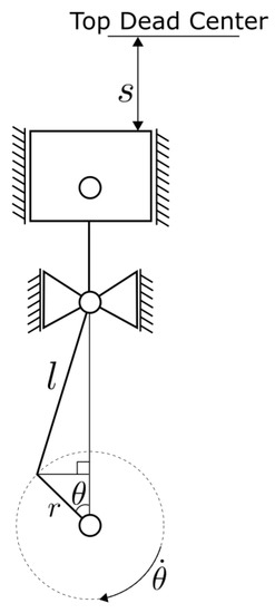
Figure 2.
Crank-slider mechanism of large two-stroke engine.
2.2.2. Mass Torque
Considering the variable inertia-speed approach, the mass torque corresponding to each engine cylinder is calculated by the following equation, which is derived by considering the kinetic energy of each cylinder rotating and reciprocating masses [39]:
where is the reciprocating mass for each cylinder, J is the moment of inertia of the rotating mass for each cylinder, and with are the crankshaft rotational speed and acceleration, respectively, at the cylinder DOF.
Equation (5) demonstrates significant non-linearities attributed to the varying angular speed and acceleration. By considering the constant-inertia speed approach, the following simplifying assumptions can be made. Firstly the instantaneous rotational speed is assumed as constant, and equal to its average value within one crankshaft revolution. Secondly, the variable inertia term (second term on the right hand side) in Equation (5), which is proportional to the angular acceleration, is also assumed constant and equal to its average value within one crankshaft revolution. Consequently, Equation (5) is simplified according to the following formula [11]:
2.2.3. Load Torque
The expression of the load torque is dependent on the type of load driven by the engine shafting system. As two stroke engines are most often employed for either ship propulsion or power generation, the engine load is either derived using the propeller law [42], or considered as a constant [27], according to the following equations, respectively:
where is the power at MCR, is the engine speed at MCR, is the propeller law exponent [42], and denotes the torque at MCR. Considering that the case of the reference study is a two-stroke diesel engine generator set, Equation (8) will be employed for the calculation of the load torque.
2.2.4. Crankshaft Dynamics Governing Equation
In order to derive the crankshaft dynamics governing equation in a matrix form, two matrices need to be considered in addition to the equations provided above. The first matrix is the cylinder selection matrix [11]. This is a matrix (where is the number of cylinders), which consists of unit elements in every location () corresponding to the the DOF and the cylinder, and zeros in all the other elements. Therefore the mathematical notation is:
A detailed derivation of for the reference system is provided in Appendix C. The above matrix is therefore used as a multiple of the combustion gas torque and mass torque functions in order to correspond their outputs to their respective cylinders.
The second matrix is the cylinder phase angle vector, which contains the phase angle of each cylinder according to the engine firing order:
The cylinder selection and phase angle matrices are used to convert Equations (3)–(8) in a matrix format, which are then substituted into Equation (2). By rearranging the resultant equation terms appropriately, Equation (11) is derived representing the crankshaft dynamics model governing equation in matrix format. The detailed description of the matrices structure is provided in Appendix B, Appendix C and Appendix D:
For the variable inertia-speed approach, and in Equation (11) are calculated according to the following equations:
Whereas the following equations are used for the constant inertia-speed approach:
2.3. Engine Friction Submodels
In this study, three different friction models of various complexity levels are employed for the calculation of each engine cylinder friction torque. The most simplistic submodel employs the constant engine friction, according to which the engine friction is taken as constant over the entire engine cycle (corresponding to one engine revolution for the two-stroke engines). In addition, it is assumed that the engine friction torque acts only on the DOF corresponding to the chaindrive, and the friction in all other DOFs is be assumed negligible. The friction torque is therefore calculated by performing the torque balance considering the sum of the average torque due to combustion for all cylinders over the complete engine cycle, and subtracting the generator load over a complete engine rotation at steady state:
The friction torque is subsequently integrated into Equation (11) as a vector of the following format:
The second engine friction submodel requires a-priori information, which is provided as friction coefficients, typically obtained from the manufacturer [10]. The engine friction at each DOF is then calculated by the product of the respective friction coefficient and the engine instantaneous rotational speed. In other words, this submodel considers the friction in the form of absolute damping, according to the following equation:
The most complex friction submodel employs an approach to estimate the instantaneous friction of each engine cylinder based on semi-empirical equations, developed by [43]. This approach was followed by [10] for calculating the friction torque of the reference system considered in this study. Specifically, the engine friction torque of each cylinder is a function of the cylinder crank angle and rotational speed and displacement , consisting of the following four components: (a) ring viscous lubrication, (b) ring mixed lubrication, (c) piston skirt and crosshead plate viscous lubrication, and (d) bearings friction. The engine friction torque function that acts as an input to the crankshaft dynamics model for the most complex engine friction submodel investigated in this study is presented in Section 2.7.
The torque exerted on the chaindrive is assumed as constant during one engine crankshaft revolution; it can be hence determined by using the following equation, which is derived through the torque balance of the entire system:
The friction torque matrix is calculated according to the following equation, which consists of two components; the first provides the instantaneous engine cylinders friction torque and is angle-dependent, whereas the second represents the constant friction torque of the chaindrive friction:
2.4. Numerical Schemes
The crankshaft dynamics governing equation (Equation (11)), as derived in Section 2.2.4, is a second order system of non-linear ordinary differential equations, with variable inertia and non-linear damping coefficients. From pertinent applications found in the literature, it is inferred that the system of differential equations is either moderately or highly stiff [11,28,31,44]. Consequently, by considering the stiffness characteristics of the investigated system, it can be deduced that the implicit numerical schemes tend to exhibit improved performance, however requiring additional computational cost [45].
The ODE23tb default solver in MATLAB [46] is a well established implicit numerical scheme used for stiff problems [47] that is appropriate for the solution of the investigated system’s governing equation. This numerical scheme uses an internally derived variable time step and implements an implicit Runge–Kutta method with trapezoidal rule integration for its first stage, and a backward differentiation formula as its second stage [48]. The ODE23tb solver also accommodates a variable inertia matrix and is the highest order stiff solver available in MATLAB, which will benefit the accuracy of the solution, however at the cost of requiring a longer computational time [47]. In addition to the above, a numerical scheme that has been successfully used for crankshaft dynamics models in automotive engine applications, approximates the crankshaft dynamics governing equation as a discrete Linear Time-Invariant (LTI) system, which has a known analytical solution [11]. Specifically, the LTI numerical scheme can successfully capture the crankshaft dynamics model complexities as it approximates the model governing equations with an LTI system for a user defined time step. Subsequently, the generated solution from each time step is employed as the initial conditions for the next time step. The advantages of this method include the low computational cost (which is suitable for real time simulations) and a highly customisable algorithm [11]. This scheme, however, comes at the cost of possible inaccuracies in the modelled response due to the approximation of the crankshaft dynamics governing equation with an LTI system and due to the explicit format of this numerical scheme [49].
2.4.1. ODE23tb Numerical Scheme
The ODE23tb numerical scheme consists of two stages for every time step [48]. Specifically, to integrate an equation of the format , such as Equation (27), the solution is firstly advanced from to using the trapezoidal rule according to Equation (21), and secondly advanced from to using a backward differentiation formula according to Equation (22).
The value of is chosen to be , such that the local truncation error is minimised [48]. The trapezoidal and backward differentiation formulae are implicit equations regarding the variables of and , respectively, and are therefore solved using an iterative approach (e.g., Newton–Raphson).
The time step is dynamically adjusted by monitoring the pointwise normalised error fraction , which is calculated according to the following equation by using the local truncation error along with the absolute and relative tolerances and set by the user:
If , then a candidate time step for the next iteration is chosen as , whilst if then .
2.4.2. Piecewise Linear Time-Invariant Numerical Scheme
The investigated crankshaft dynamics model governing equation (Equation (11)), which is nonlinear, can be approximated at every time step by the following LTI system equation [50]:
The LTI numerical scheme employs Equation (26) for the calculation of the state variable at the time step, by assuming that remains constant for this time step, and by discretising Equation (25) using the trapezoidal rule.
where is the identity matrix.
To determine the matrices and as well as the vector , the crankshaft dynamics model governing equation (Equation (11)) needs to be transformed to its state-space representation. By letting , the following equation is derived:
where:
Having calculated the state vector (), the torque between subsequent DOFs is calculated by Equation (28). It must be noted that this equation is used from both numerical schemes.
2.4.3. Convergence Criterion and Time Step Study
For the implementation of both numerical schemes, it is important to determine a convergence criterion, which is used to characterise the system steady state response and terminate the simulation run (when required). In this study, the Normalised Root Mean Square Error (NRMSE) of the flywheel instantaneous torque considering two consecutive engine shaft revolutions is employed. Specifically, the NRMSE for the predicted flywheel torque response of the engine revolution is calculated according to the following equation:
where n denotes the total number of elements in the predicted flywheel torque response for every engine revolution.
Hence, due to the periodicity of the torque response, as the solution settles to its Steady State (SS), it is expected that the NRMSE between two successive engine revolutions will approach zero [10]. Consequently, the solution converges after the NRMSE has decreased below a threshold , which is determined in Section 3.1. Once the convergence criterion is satisfied, the model output that includes the flywheel torque at the last engine revolution is considered as the SS solution. The employed model flowchart is shown in Figure 3.
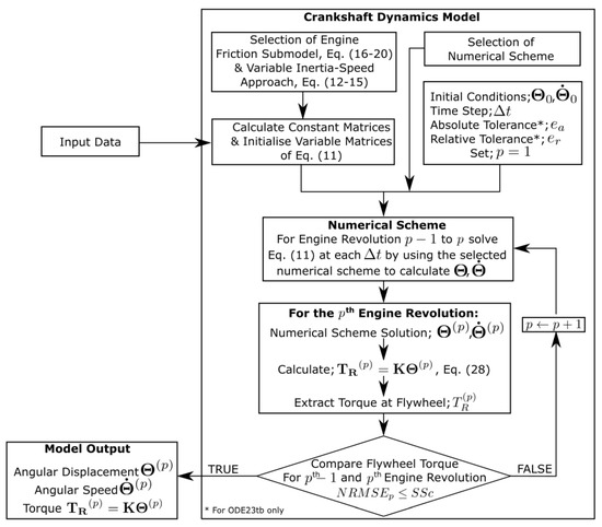
Figure 3.
Crankshaft dynamics model flowchart. For the description of the Input Data refer to Figure 4. The matrices with superscript p horizontally concatenate the vectors from the governing equation solution for every time step included in the engine revolution.
The time step study will take place only for the LTI numerical scheme, as the ODE23tb time step is internally derived and adjusted within the MATLAB algorithm. The procedure involves running the LTI numerical scheme for a range of time step values and for every SS solution, the NRMSE is calculated by considering the modelled and the measured torque response at the flywheel ( and , respectively), using the following equation:
Numerical analysis theory dictates that for a stable numerical scheme, as the time step decreases, the NRMSE between the modelled and measured torque response at the flywheel must asymptotically approach a constant value [51]. Consequently, the time step is selected, so that both the NRMSE and the computational cost are considered acceptable.
2.5. Key Performance Indicators for Systematic Comparison
In this study, three KPIs are considered for systematically comparing the investigated case studies solutions characteristics. The first KPI is the NRMSE between the derived SS solution and measured torque response at the flywheel, as calculated by Equation (30). This indicates the accuracy of the model by considering the available measured data.
The second KPI is the computational time required by the crankshaft dynamics model to obtain a steady state convergence. This is an important performance indicator due to the potential use of the model for online/real-time torque prediction and engine diagnosis [11,23,29].
The third KPI is the Euclidean norm of the energy balance error throughout one engine revolution at SS conditions. The energy balance KPI represents a multitude of parameters, which affect the performance of the crankshaft dynamics model. Specifically, the extent to which the energy balance is satisfied throughout one engine revolution depends firstly on the numerical scheme and the associated discretisation errors it introduces, secondly on the computational device employed and the round-off errors it introduces [51], and thirdly on the simplifying assumptions made (if any) in the crankshaft dynamics governing equations.
The energy balance equation of the investigated system consists of three terms. The first is the sum of the kinetic and potential energies for each DOF, , the second is the dissipated energy due to the engine load as well as the system damping and friction, , and the third is the transferred energy on the piston due to each combustion event, . These parameters are described from the following equations:
The energy balance error of the modelled system’s solution, which must ideally be zero at each time step, is calculated by using the following equation:
where denotes the system total initial energy (kinetic and potential) obtained from the initial conditions provided at the start of the simulation run. The Euclidean norm of the energy balance error is then defined according to the following equation:
The summary of the three considered KPIs is listed in Table 1.

Table 1.
Considered Key Performance Indicators (KPIs) summary.
2.6. Systematic Comparison Procedure
For the systematic comparison to be carried out in this study, various combinations of the crankshaft dynamics models alternatives will be investigated. Specifically, as listed in the beginning of Section 2, these alternatives are the two numerical schemes, the constant and variable inertia-speed approaches, as well as the three engine friction submodels. Consequently, twelve different case studies are required in order to examine the performance of the crankshaft dynamics model for all possible combinations of the above alternatives; these case studies are listed in Table 2.
Table 2.
List of case studies.
To quantify the overall performance for each case study, the three KPIs as listed in Section 2.5 are utilised to calculate the total Performance Measure (PM) according to Equation (36). Specifically, the PM includes of the NRMSE with the measured data (denoted as ), the computational time (denoted as ), and the Eucledian norm of the energy balance error (denoted as ), which are normalised by determining their respective maximum value from all 12 case studies. Subsequently, the normalised KPIs are summed to obtain the total PM for each case study. By employing the above procedure, all KPIs are considered to have equal importance in the calculation of the PM.
where the overline in this context represents a normalised value.
Consequently, the crankshaft dynamics model case study with the lowest PM value is the best performing, whilst the case study with a PM value closest to three is the worst performing. The advantage of using Equation (36) is that a concise summary of the best performing case study is obtained by directly comparing the results for all KPIs; however, the physical interpretation of these results cannot be obtained.
Therefore, physical insight can be acquired by comparing the non-normalised KPIs and the predicted torque of specific case studies. Specifically, the non-normalised KPIs comparison will provide insight as to which KPI is responsible for the improved performance of the crankshaft dynamics model. Moreover, the NRMSE with the measured data KPI considers the torque of the reference system only between the flywheel and the generator (DOFs 15–16); thus, it is prudent to examine the derived simulation results in other DOFs as well. Hence, a representative sample from the response in all DOFs can be obtained by considering the predicted torque between cylinders 1 and 2 (DOFs 4–5) as well as between the chaindrive and cylinder 6 (DOFs 9–10). Therefore, according to the above, a total of three locations on the crankshaft are examined, at the three crankshaft locations of cylinder 1, chaindrive, and flywheel.
As there is no measured data to facilitate a comparison at the aforementioned DOFs, the results will be compared by utilising the NRMSE with the solution of case study 12, thereafter referred to as the reference case study. This is considered as the reference case study since it employs the well established ODE23tb numerical scheme, and in theory it represents the reference system more closely, as it makes the fewest assumptions and approximations compared to all other case studies by utilizing the variable engine friction submodel and the variable inertia-speed approach.
By considering the above, the systematic comparison procedure is developed as follows:
- Determination of the overall best performing crankshaft dynamics model by comparing case studies 1–12 via the PM.
- Comparison of selective case studies via the non-normalised KPIs:
- (a)
- Comparison of the engine friction submodels to determine the best performing submodel. This is performed by considering the crankshaft dynamics model with the variable inertia-speed approach for both numerical schemes; hence, the results of the case studies 2, 4, 6, 8, 10, and 12 (Table 2) are compared. For this comparison, the variable inertia-speed approach was used as it represents the real physical system more closely compared to the constant inertia-speed approach, which includes simplifications.
- (b)
- Comparison of the inertia-speed approaches considering the crankshaft dynamics model with the best performing engine friction submodel as determined in the previous step. This comparison is performed for both numerical schemes. Hence, the simulation results for the following case studies are compared:
- i
- If the constant engine friction submodel is the best performing: case studies 1, 2, 7, 8 are compared.
- ii
- If the coefficients matrix engine friction submodel is the best performing: case studies 3, 4, 9, 10 are compared.
- iii
- If the variable engine friction submodel is the best performing: case studies 5, 6, 11, 12 are compared.
- Comparison of the selected case studies listed below via the NRMSE, with the measured torque data or the reference case study (case study 12) where applicable, at the locations of cylinder 1, chain drive, and flywheel:
- (a)
- Numerical schemes comparison, by considering the most complex crankshaft dynamics model with the LTI numerical scheme (case study 6).
- (b)
- Engine friction submodel comparison, by considering the ODE23tb numerical scheme and the variable inertia-speed approach (case studies 8 and 10).
- (c)
- Inertia-speed approaches comparison, by considering the ODE23tb numerical scheme and the best performing engine friction submodel. Hence, the simulation results for the following case studies are compared:
- i
- If the constant engine friction submodel is the best performing: case studies 7 and 8 are compared.
- ii
- If the coefficients matrix engine friction submodel is the best performing: case studies 9 and 10 are compared.
- iii
- If the variable engine friction submodel is the best performing: case studies 11 and 12 are compared.
2.7. Crankshaft Dynamics Model Input Data and Assumptions
The input, output, and assumptions of the developed crankshaft dynamics model and the investigated alternatives are discussed in this section. The input of the model consists of parameters that can be grouped into the five categories of; (a) DOF coefficients, (b) in-cylinder pressure diagram, (c) generator load torque, (d) validation data, and (e) geometric and other data. The model output includes the angular displacement and speed in each DOF as well as the torque in the shafting system parts between two adjacent DOFs. The flywheel ICT (which is the torque between DOF 15 and 16) is used for the model results validation, as illustrated in Figure 4.
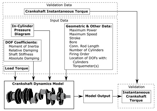
Figure 4.
Engine crankshaft dynamics model input and output parameters.
The DOF coefficients include the moment of inertia, the relative damping, and the shaft stiffness coefficients, which form the matrices , , and in Equation (11). The relative damping coefficient forms the matrix of the coefficients matrix friction submodel (Equation (18)). The matrix coefficient values are presented in Appendix A. A limitation with regards to the usage of the coefficient matrices is that they are obtained from the manufacturer when the engine is in a new condition. Consequently, any subsequent engine degradation that results in changes of these coefficients values cannot be taken into account, unless these coefficients are re-calculated to reflect on the current engine condition.
The in-cylinder pressure, the generator load torque, the measured engine flywheel ICT (used for the model validation) and the cylinder friction torque for 100% MCR, were taken from [10,27] and are shown in Figure 5. The in-cylinder pressure is used as input to calculate the gas torque (Equation (3)), whereas the generator load torque is used as input in Equation (8). The ICT measured data is employed for the calculation of the KPIs (described in Section 2.5) and the validation of the model in Section 3.1. As the in-cylinder pressure data is only available for one cylinder, it was assumed that the pressure is identical for all engine cylinders. In addition, it is assumed that the pressure diagram and the ICT data measurements were taken at a synchronous time, although this is highly unlikely, as the in-cylinder pressure diagrams are taken as average over several engine cycles. Nevertheless, the differences between the available measurements and the actual parameters are expected to be small. Finally, the cylinder friction torque was used as input to for the most complex engine friction submodel (Equation (19)).
Figure 5.
Reference system data of (a) in-cylinder pressure, (b) Instantaneous Crankshaft Torque (ICT), and (c) engine friction, all for 100% MCR at 13.8 MW load from [10].
The geometric and other data used as input parameters in the model are listed in Table 3. These parameters are employed for the calculations according to Equations (3)–(6) as well as to determine the cylinder phase angle vector according to Equation (10).
Table 3.
Reference engine basic characteristics [27].
3. Results and Discussion
3.1. Crankshaft Dynamics Model Time Step Study
As mentioned in the Methodology section, the time step study for the LTI numerical scheme has to be performed, as the ODE23tb scheme employs an algorithm for the time step determination. The convergence criterion is the metric used to end the simulation run of the engine crankshaft dynamics model, by considering that steady state operating conditions are established. This is determined by employing the NRMSE between successive engine revolutions to identify the system SS conditions. The case studies 6 (variable inertia-speed approach, most complex friction submodel and LTI scheme) and 12 (variable inertia-speed approach, most complex friction submodel and ODE23tb scheme) were investigated and the derived results are presented in Figure 6. For case study 6, different time steps were employed. It is observed that the , after 4∼5 engine revolutions, consistently remains below 0.5% for both solvers and at time steps smaller than 3 ms for the LTI scheme. Therefore, the recommended convergence criterion for the investigated system crankshaft dynamics model is the equal to 0.5%.
Figure 6.
Case studies 6 and 12 results: versus time step for case study 6 (variable inertia- speed approach, most complex friction submodel and Linear Time-Invariant (LTI) scheme); for case study 12 (variable inertia-speed approach, most complex friction submodel and ODE23tb scheme).
Having established the convergence criterion, the recommended time step can be determined for the LTI numerical scheme. In this case, the crankshaft dynamics model runs were performed for a series of time step values for the case studies 5 and 6, which pertain to both the constant and variable inertia-speed approaches, and they were terminated when the convergence criterion determined above was achieved. From the results shown in Figure 7, it is observed that the between the modelled and measured flywheel torque response for time steps less than 3 ms remains at approximately 8%. Specifically, as the time step gets smaller the increase in computational time is substantial in contrast to the decrease in , which remains negligible. Hence, it can be concluded that the recommended time step for the LTI numerical scheme is 3 ms. The results of the time step study and determination of the convergence criterion, are listed in Table 4.
Figure 7.
LTI numerical scheme time step investigation.
Table 4.
Convergence criterion and time step study recommendations.
3.2. Crankshaft Dynamics Model Validation
The crankshaft dynamics model is validated by employing the convergence criterion and the recommended time step to predict the flywheel torque response for the case studies 6 (variable inertia-speed approach, most complex friction submodel and LTI scheme) and 12 (variable inertia-speed approach, most complex friction submodel and ODE23tb scheme). Considering the derived simulation results and the respective measured data, the values for each case were calculated. The derived torque responses along with the respective measured data and values are presented in Figure 8.
Figure 8.
Variable engine friction submodel and variable inertia-speed approach predicted torque (case studies 6 and 12).
The modelled torque response for both case studies provides adequate accuracy compared with the measured data, as the values for the LTI and ODE23tb numerical schemes were found to be 8.10% and 8.74%, respectively. Therefore, it can be deduced that the simulation results (flywheel torque) error is approximately the same for both case studies, which share identical model inputs and governing equations.
Hence, it can be inferred that the source of this error is either the model inputs, or crankshaft dynamics model governing equations, which require increased complexity or alternative formulation to better capture the rotational motion of the shafting system. The latter is highly unlikely as the equations have been derived from first principles and extensively studied in the literature [10,11,39]. The former is more likely, for reasons also mentioned in Section 2.7. Specifically, the coefficient matrices were obtained from the manufacturer corresponding to the engine at new condition, so subsequent engine degradation that results in changes in these coefficients values was not taken into account. Most importantly, the in-cylinder pressure diagram was available for only one cylinder, so it was assumed that the in-cylinder pressure was identical for all the engine cylinders, which most certainly is not always the case [10,29]. Finally, the variable engine friction submodel applied to every cylinder may require calibration in its parameters, which would result in improved accuracy of the NRMSE with the measured data.
3.3. Crankshaft Dynamics Model Performance Systematic Comparison
3.3.1. Performance Measure (PM)
Simulation runs were performed for all the case studies (1–12); the derived results were used to calculate the three KPIs and the PM. The derived results for PM are summarised in Figure 9. From these results, it is deduced that the case studies 7 (constant engine friction, constant inertia-speed and ODED23tb scheme) and 9 (coefficients matrix engine friction, constant inertia-speed and ODED23tb scheme) exhibited the best performance with nearly identical PM values (1.60 and 1.59, respectively). The case studies 4 and 2 (variable inertia-speed with LTI numerical scheme) also exhibit low PM values (1.85 and 1.79, respectively), which indicates that the two most simplistic engine friction submodels result to the best performing case studies. In order to gain physical insight and interpret the significance of these results, the KPIs of selective case studies are compared in the next section.
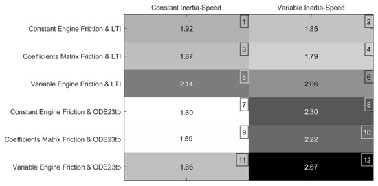
Figure 9.
Derived performance measure values for the investigated case studies 1–12.
3.3.2. Key Performance Indicators (KPIs)
As described in Section 2.6 (step 2a), the three KPIs calculated for the case studies 2, 4, 6, 8, 10, 12 are compared, as shown in Figure 10a–c. It is observed that derived results for the KPI 1 () were found to be in the range 7.5–8.3, with the higher values corresponding to the case studies 8, 10, and 12 (employing the ODE23b scheme). The calculated values demonstrate an adequate agreement of the derived results with the measured flywheel torque data, which also indicates that the acceptable model validation for the investigated cases (as discussed in the preceding section). Considering the influence of the friction submodel, it is deduced that the coefficients matrix friction resulted in the lowest values (cases 4 and 10 with the LTI and ODE23tb schemes, respectively). The other friction submodels exhibited slightly higher values, which, however, were found to be very close to each other.
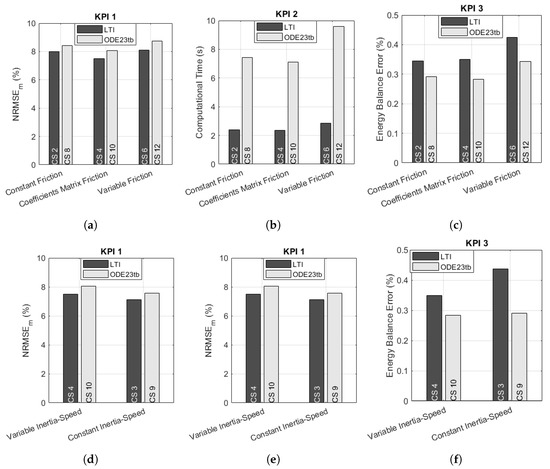
Figure 10.
Engine friction submodel comparison of (a) KPI 1, (b) KPI 2 and (c) KPI 3. Inertia-speed approaches comparison of (d) KPI 1, (e) KPI 2, and (f) KPI 3.
Considering the KPI 2 (computational time) shown in Figure 10b and by comparing the case studies 2, 4, and 6 (with the LTI scheme) as well as the case studies 8, 10, and 12 (with ODE23tb scheme), it is observed that the case studies 4 and 8 employing the coefficients matrix friction submodel exhibited the lower computational time (for each numerical scheme), although the computational time required for the case studies 2 and 8 was comparable. The longer computational time was observed for the variable engine friction model for the case studies 6 and 12 ( s and s, respectively). As expected, the case studies 8, 10, and 12 (employing the ODED23tb scheme) required the longer computational time (in comparison with the respective cases employing the LTI scheme), with the case study 12 exhibiting the longest computational time among all cases.
Comparing the KPI 3 values (energy balance error), it is inferred that the case study 10 exhibited the lowest value among all the cases employing the ODE23tb scheme, whereas the case study 2 provided this KPI lowest value among the cases employing the LTI scheme. However, the values observed for the case studies 10 and 4 were very close compared with the obtained lowest values for the ODE23tb and LTI numerical schemes. The derived energy balance errors were greater for the LTI numerical scheme. The highest values for this KPI were obtained for the case studies 6 and 12 with the LTI and the ODE23tb schemes, respectively.
These derived results confirm, as expected, that a greater computational effort is required for the most complex engine friction submodel. In addition, they also signify that this submodel may require better calibration of its parameters as the energy balance error was higher for the case study 12 with the most complex friction submodel as compared to the other two case studies with the most simplistic engine friction submodels.
When comparing the two numerical schemes for all case studies in Figure 10a–c, it is observed that the case studies with the LTI scheme exhibited a much faster computational time. However, by considering the and the energy balance error KPIs, both numerical schemes seem to have only a small effect in the flywheel ICT prediction accuracy. Nonetheless, it must be noted that the energy balance error for the case of the ODE23tb is consistently lower from the case study with the LTI scheme, which signifies that the ODE23tb is a much more effective numerical scheme in terms of numerical error. However, the effect this bears in the model accuracy when compared to the measured flywheel torque remains negligible, as deduced from the first KPI values presented in Figure 10a.
Therefore, by considering the PM values from Figure 9, it is concluded that the coefficients matrix engine friction submodel performs the best for both the LTI and ODE23tb numerical schemes, as demonstrated by the results of case studies 4 and 10. Consequently, in accordance with step 2 (in Section 2.6), the case studies 3, 4, 9, and 10 are compared. The derived KPIs are shown in Figure 10d–f.
From the derived KPI 1 results, it is observed that the for both inertia approaches are virtually identical, with their average difference between the two numerical schemes being approximately 0.4%. It was reported in [11] that the constant inertia-speed approach is as accurate as the variable inertia-speed approach for applications in automotive engines. By considering the results of this study, the same conclusion is also drawn for the large two-stroke engines. Hence, it can be inferred that the larger rotating masses and the rotational speed fluctuation do not bear any effect on the simplifying assumptions made by the constant inertia-speed approach.
Considering the derived results for the KPI 2, the computational time improvement of the constant inertia-speed approach for the LTI numerical scheme (case studies 4 and 3) is s (in comparison with the variable inertia-speed approach for the LTI scheme). However, there is a significant improvement of s for the ODE23tb numerical scheme (case studies 10 and 9). This indicates that the ODE23tb responds well to the simplifying assumptions made by the constant inertia-speed approach, since the model accuracy remains virtually the same, but the improvement in computational time is significant.
The KPI 3 (energy balance error), in the same manner as with the case studies shown in Figure 10c, has shown consistent improvement for the case studies with ODE23tb in comparison to the case studies with the LTI numerical scheme (i.e., case studies 4 vs. 10 and 3 vs. 9). This indicates that the ODE23tb numerical scheme is a more effective numerical scheme. In addition, the energy balance error for the case of the ODE23tb numerical scheme seems to be only slightly affected by the type of inertia approach used (case studies 10 and 9). This indicates once more the effectiveness of this numerical scheme. However, for the case of the LTI numerical scheme, the energy balance error slightly increases on average by 0.6% as compared to the ODE23tb numerical scheme respective results.
3.3.3. Predicted Torque at Individual Crankshaft Locations
In accordance to step 3(a) in Section 2.5, the numerical schemes are compared in Figure 11a–c by considering the most complex crankshaft dynamics model with the LTI numerical scheme (case study 6) and comparing it against the reference case study (case study 12) and the measured data where applicable. It is observed that the predicted torque of case study 6 using the recommended time step of 3 ms in the above section, significantly deviates from that of case study 12 for the cylinder 1 and chaindrive locations. As this could be considered to be an effect of the large time step, it is observed that by reducing the time step to 1 ms, the predicted response of case study 6 matches more closely that of case study 12 at the aforementioned locations. Therefore, when the response at DOFs other than the flywheel is considered, the recommended time step should be reduced to 1 ms as summarised in Table 5. However, for the case of the reduced time step, there is a high frequency oscillation introduced to the solution.
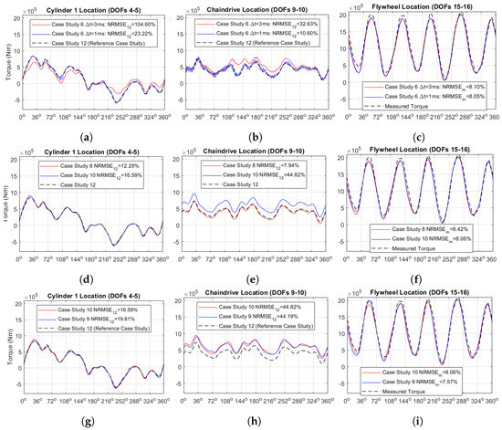
Figure 11.
Numerical schemes of LTI and ODE23tb (case studies 8, 12) torque comparison for Δt = 3 ms (recommended time step) and Δt = 1 ms at (a) cylinder 1, (b) chaindrive, and (c) flywheel crankshaft locations. Constant and coefficients matrix engine friction submodels (case studies 8, 10) torque comparison at (d) cylinder 1, (e) chaindrive, and (f) flywheel crankshaft locations. Constant and variable speed-inertia approaches (case studies 9, 10) torque comparison at (g) cylinder 1, (h) chaindrive, and (i) flywheel crankshaft locations.
Table 5.
Amended convergence criterion and time step study recommendations.
The above is an effect that is observed in highly oscillatory multi-body dynamic systems, and is due to the fact that the ODE23tb and the LTI are implicit and explicit schemes, respectively [52,53]. Specifically, it is known that as an intrinsic property of implicit schemes such as the ODE23tb, damping may be introduced in high frequency oscillations present in the solution in order to maintain stability, in a process that is referred to as under-relaxation [47]. In contrast, the explicit LTI scheme employed may be susceptible to errors being accumulated through the iterations that may artificially stimulate high frequency oscillations (such as the ones observed in this case), which could be a result of the modelling and/or numerical processes rather than the actual physics of the system [54]. From the above, since the implicit ODE23tb scheme appears to dampen the response, whilst the explicit LTI scheme appears to stimulate already existing high frequencies, it can be inferred that the realistic response of the system lies between the two extremes shown by the solutions of the ODE23tb and the LTI schemes, respectively.
In accordance to step 3(b) in Section 2.5, the engine friction submodels are compared to the measured torque and the reference case study (case study 12) results and the measured data where applicable. The derived torque variations at three locations are shown in Figure 11d–f. Considering the predicted flywheel torque variations, it is deduced that the coefficients matrix friction submodel is the most accurate when compared to the measured data, and this can be also confirmed from KPI 1 in Figure 10a. In the same manner as with the numerical scheme comparison provided in the preceding paragraphs, it is concluded that the predicted flywheel torque for all friction submodels shows sufficient agreement with the measured data, and the friction model only slightly impacts this result.
For the chaindrive location however, the coefficients matrix friction submodel results (torque variation) is offset considering the respective results from the constant and variable engine friction submodel (case studies 10 and 12), by approximately kNm. This resulted in a significant increase of that was found to be 44.82% considering the torque variations of case studies 10 and 12. This occurs since the constant engine friction model applies a constant friction torque only to the chaindrive DOF, and consequently it reduces the torque on the shaft between the chaindrive and cylinder 6. This can be confirmed as the constant friction torque applied to the chaindrive is kNm, about the same as the predicted offset. The same behaviour is observed for the variable friction model, which applies the variable friction to each cylinder, and the remaining friction from the torque balance is considered constant applied to the chaindrive. This behaviour occurs since the cylinder friction from Figure 5 has an instantaneous maximum of just kNm and an average of just kNm, which therefore makes the variable friction submodel behave similar to the constant friction submodel. Last, considering the predicted torque variations at cylinder 1 location, it is observed that there is no significant difference amongst these case studies results. Hence, it can be inferred that for improving the variable engine friction submodel performance, a more effective calibration of its parameters may be required, or the friction losses in other loaded bearings such as thrust bearings need to be taken into account more accurately.
Therefore, it can be confirmed that for the flywheel torque prediction, the engine friction submodel does not significantly affect the results, since from Figure 10a results, an improvement in the of 0.68% is obtained for the case study 10. The same holds for the cylinder 1 location where only slight differences are observed. Hence, it can be deduced that in the absence of available data, employing the constant engine friction submodel can provide sufficient accuracy for predicting the torque variations in these crankshaft locations. However, for the chaindrive location, significant differences are observed, based on which, it is inferred that the coefficients matrix friction submodel is the friction model that can provide the highest accuracy. In addition, according to Figure 10c, it also has the lowest energy balance error at 0.28%. The effective behaviour of this friction submodel is attributed to the fact that the input data for this one is obtained from the manufacturer torsional vibration study. On the contrary, the constant friction submodel oversimplifies the associated phenomena, whereas the variable friction model needs more elaborate calibration based on detailed measured data, which are rarely available.
In accordance to step 3(c), in Section 2.5, the results of the variable and constant inertia-speed approaches with the best performing engine friction submodel are compared to the measured data and the reference case study (case study 12) results (where applicable). It must be noted that the ODE23tb numerical scheme is employed in all the compared case studies. The derived torque variations are illustrated in Figure 11g–i. The constant and variable inertia-speed approaches (case studies 9 and 10), exhibit virtually identical responses in the crankshaft locations of cylinder 1 and flywheel. For the chaindrive, as expected, an offset in the predicted torque is exhibited between the case studies 9 and 10 results and the reference case study results, due to the different employed engine friction submodels. This was discussed in detail in the preceding paragraph. When compared to each other for the three crankshaft locations, case studies 9 and 10 results exhibited a maximum NRMSE difference of just 0.63%, hence it can be concluded that the analysis in Section 3.3.2 provides sufficient insight.
In summary, the crankshaft dynamics model was validated (based on the adequate prediction of the measured torque data), and its performance was investigated. This was accomplished by choosing the best performing options regarding the engine friction submodel, the constant vs. variable inertia-speed approach, and the numerical schemes employed. Hence, in accordance to the metrics developed in this study, the best performing crankshaft dynamics model for large two-stroke engines employs the ODE23tb solver, the constant inertia-speed approach, and the coefficients matrix engine friction submodel, as summarised in Table 4. In addition to the above, it was demonstrated that the much simpler LTI scheme offers comparable performance to the ODE23tb scheme considering the KPIs 1 and 3 whilst exhibiting much lower computational cost. The same holds for the constant engine friction submodel considering its simplicity and the lack of input data requirements, as it offers adequate accuracy (demonstrated by the case studies 1 and 2 results).
4. Conclusions
This study focused on the systematic investigation of the crankshaft dynamics model performance for a two-stroke diesel engine. This was accomplished by quantifying the model performance through a series of Key Performance Indicators (KPIs), which were included in an overall Performance Measure (PM) such that smaller PM values indicate better performance. Subsequently, the PM was examined through specific case studies, which included two alternative numerical schemes, the constant and variable inertia-speed approaches and three different engine friction submodels of varying complexity. The main findings of this study are summarised as follows.
Considering the predicted and measured engine flywheel torque, it was concluded that the large two-stroke diesel engine crankshaft dynamics model employing the ODE23tb numerical scheme, the constant inertia-speed approach and the coefficients matrix engine friction submodel was the best performing alternative exhibiting a PM of 1.59.
Although the ODE23tb numerical scheme provided the best overall performance, the Linear Time-Invariant (LTI) numerical scheme displayed satisfactory accuracy with significant computational time savings of approximately 70%, for all case studies comparing the engine friction submodels. However, it was found that the LTI numerical scheme requires a smaller time step to predict with sufficient accuracy the torque at the parts of the engine crankshaft, and it introduces a prominent high frequency oscillation to the derived solution, which is attributed to the explicit nature of the LTI numerical scheme. Therefore, by considering its mathematical and computational simplicity, the LTI numerical scheme use would be recommended for applications in large two-stroke engines in cases where the aim is to predict the flywheel torque.
The constant inertia-speed approach as compared to the variable inertia-speed approach exhibited small differences in the predicted results accuracy, when examining the predicted torque at cylinder 1, chaindrive, and flywheel locations. Most importantly, the constant inertia-speed approach demonstrated significant computational time savings in the order of 80% for the case of the ODE23tb numerical scheme. Therefore, considering that the reference system is a constant speed engine, the use of this approach would be recommended. However for the model application in two stroke marine engines for ships propulsion, unless the focus is placed on a specific operating point, the variable inertia-speed approach would be recommended in order for the crankshaft dynamics model to be able to address the entire engine operating envelope.
Finally, the choice of the engine friction submodel had a small effect on the model output when considering the predicted flywheel torque. The constant engine friction submodel demonstrated significant time savings, however when examining the chaindrive Degrees of Freedom (DOFs), a significant difference was exhibited between the results of this model and the results of the best performing coefficients matrix engine friction submodel. Moreover, the variable engine friction submodel required better calibration for taking into account the frictional forces in other loaded bearings in order to match in accuracy the results of the best performing friction submodel at the chaindrive DOF. Hence, it would be recommended to use the simplest friction submodel for the cases where the focus is on the flywheel torque prediction and in absence of more detailed data. However, a more intensive approach would be required for predicting the torque at other DOFs with sufficient accuracy.
In conclusion, this study successfully implemented a systematic investigation in the crankshaft dynamics model of a large two-stroke diesel engine, which identified advantages and disadvantages of the crankshaft dynamics model main features, such that the best performance can be obtained. This has laid the foundation for the efficient prediction of the Instantaneous Crankshaft Torque (ICT) for such engines, and most importantly has established a robust relationship between the engine thermodynamic processes (i.e., in-cylinder pressure) and its torque output, which in future work will be used for failure identification and diagnostics.
Author Contributions
Conceptualization, K.-M.T. and G.T.; methodology, K.-M.T. and G.T.; software, K.-M.T.; validation, K.-M.T., G.T., N.X. and M.H.; formal analysis, K.-M.T. and G.T.; resources, G.T. and M.H.; data curation, K.-M.T.; writing—original draft preparation, K.-M.T. and G.T.; writing—review and editing, K.-M.T., G.T., N.X. and M.H.; visualization, K.-M.T.; supervision, G.T. and M.H.; funding acquisition, G.T. and M.H. All authors have read and agreed to the published version of the manuscript.
Funding
The authors gratefully acknowledge the financial support of Innovate UK, through the Knowledge Transfer Partnership project (project number 11577), for the work reported in this article.
Acknowledgments
The authors from MSRC greatly acknowledge the funding from DNV GL AS and RCCL for the MSRC establishment and operation. The opinions expressed herein are those of the authors and should not be construed to reflect the views of Innovate UK, DNV GL AS and RCCL.
Conflicts of Interest
The authors declare no conflict of interest.
Abbreviations
The following abbreviations are used in this manuscript:
| DOF | Degree of Freedom |
| ICT | Instantaneous Crankshaft Torque |
| ICS | Instantaneous Crankshaft Speed |
| KPI | Key Performance Indicator |
| LTI | Linear Time-Invariant |
| MCR | Maximum Continuous Rating |
| NRMSE | Normalised Root Mean Squared Error |
| PM | Performance Measure |
| SS | Steady State |
Appendix A. Reference System Coefficients
The reference system stiffness, inertia, relative damping, and absolute damping coefficients utilised as input to the crankshaft dynamics model are shown in Table A1 below:
Table A1.
DOF Coefficients obtained from [10].
Table A1.
DOF Coefficients obtained from [10].
| DOF | Stiffnes | Inertia | Rel. Damping | Abs. Damping |
|---|---|---|---|---|
| (kg m) | (Nms/rad) | (Nms/rad) | (Nms/rad) | |
| 1 | 1.00 | 8.54 | 5.70 | 0 |
| 2 | 1.00 | 4.48 | 0 | 0 |
| 3 | 1.34 | 4.42 | 0 | 0 |
| 4 | 1.20 | 6.52 | 5.00 | 2.29 |
| 5 | 1.20 | 6.89 | 5.00 | 2.29 |
| 6 | 1.20 | 6.52 | 5.00 | 2.29 |
| 7 | 1.21 | 6.62 | 5.00 | 2.29 |
| 8 | 1.30 | 6.89 | 5.00 | 2.29 |
| 9 | 1.41 | 3.81 | 5.00 | 2.29 |
| 10 | 1.21 | 6.89 | 5.00 | 2.29 |
| 11 | 1.20 | 6.89 | 5.00 | 2.29 |
| 12 | 1.20 | 6.52 | 5.00 | 2.29 |
| 13 | 1.20 | 6.90 | 5.00 | 2.29 |
| 14 | 8.15 | 6.52 | 0 | 2.29 |
| 15 | 6.93 | 3.06 | 0 | 3.29 |
| 16 | 5.94 | 8.54 | 1.45 | 2.69 |
Appendix B. Reference System Coefficient Matrices
The stiffness and damping coefficient matrices utilised in the crankshaft dynamics governing equation (Equation (11)) both have the same format. Specifically, assuming a vector of coefficients , the following would be its equivalent damping or stiffness matrix in sparse format:
Regarding the inertia and absolute damping coefficients by considering generic coefficient values , these matrices are diagonal:
Appendix C. Cylinder Selection Matrix
The cylinder selection matrix is of size , with its number of rows and columns corresponding to the number of DOFs and cylinders, respectively. The matrix elements equivalent to unity correspond to the location of each cylinder, for example:
- The 4th DOF corresponds to the 1st cylinder, hence .
- The 5th DOF corresponds to the 2nd cylinder, hence .
- ⋮
- The DOF corresponds to the cylinder, hence .
Therefore, for the reference system, the cylinder selection matrix has the format shown in Equation (A3) below:
Appendix D. Governing Equations of Crankshaft System
The torque balance in matrix form as shown in Equation (2) is as follows:
By employing the equations derived in Section 2, the individual terms of the above equation can be derived in matrix format for the variable inertia-speed approach as follows:
where:
- and correspond to the variable and constant inertia-speed approach respectively.
- , with defined in Equation (4).
- , with p being the in-cylinder pressure as a function of crank angle.
- defined as the element-wise derivative of .
- defined as the element wise multiplication of the respective matrix with itself.
By substituting the Equations (A5)–(A9) into Equation (A4) and rearranging appropriately, this would result in Equation (11) as shown in Section 2.2.4.
References
- Mattarelli, E.; Cantore, G.; Rinaldini, C.A. Advances in the Design of Two-Stroke, High Speed, Compression Ignition Engines; IntechOpen: London, UK, 2013. [Google Scholar]
- Okabe, M.; Sakaguchi, K.; Sugihara, M.; Miyanagi, A.; Hiraoka, N.; Murata, S. World’s largest marine 2-stroke diesel test engine, the 4UE-X3-development in compliance with the next version of environmental regulations and gas engine technology. Mitsubishi Heavy Ind. Tech. Rev. 2013, 50, 55. [Google Scholar]
- Reynaert, M. Abatement Strategies and the Cost of Environmental Regulation: Emission Standards on the European Car Market; CEPR Discussion Paper No. DP13756; SSRN: Rochester, NY, USA, 2019. [Google Scholar]
- Van, T.C.; Ramirez, J.; Rainey, T.; Ristovski, Z.; Brown, R.J. Global impacts of recent IMO regulations on marine fuel oil refining processes and ship emissions. Transp. Res. Part D Transp. Environ. 2019, 70, 123–134. [Google Scholar] [CrossRef]
- Stanton, D.W. Systematic development of highly efficient and clean engines to meet future commercial vehicle greenhouse gas regulations. SAE Int. J. Engines 2013, 6, 1395–1480. [Google Scholar] [CrossRef]
- Woodyard, D. Pounder’s Marine Diesel Engines and Gas Turbines, 9th ed.; Butterworth-Heinemann: Oxford, UK, 2009. [Google Scholar]
- Llamas, X.; Eriksson, L. Control-oriented modeling of two-stroke diesel engines with exhaust gas recirculation for marine applications. Proc. Inst. Mech. Eng. Part M J. Eng. Marit. Environ. 2019, 233, 551–574. [Google Scholar] [CrossRef]
- Theotokatos, G.; Guan, C.; Chen, H.; Lazakis, I. Development of an extended mean value engine model for predicting the marine two-stroke engine operation at varying settings. Energy 2018, 143, 533–545. [Google Scholar] [CrossRef]
- Romero, C.; Piedrahita, R.; Fabio, H.; Riaza, Q. Prediction of In-Cylinder Pressure, Temperature, and Loads Related to the Crank Slider Mechanism of I. C. Engines: A Computational Model; SAE Technical Paper; SAE International: Warrendale, PA, USA, 2003. [Google Scholar] [CrossRef]
- Guerrero, D.P.; Jiménez-Espadafor, F.J. Torsional system dynamics of low speed diesel engines based on instantaneous torque: Application to engine diagnosis. Mech. Syst. Signal Process. 2019, 116, 858–878. [Google Scholar] [CrossRef]
- Schagerberg, S.; Mckelvey, T. Instantaneous Crankshaft Torque Measurements—Modeling and Validation; SAE Technical Papers; SAE International: Warrendale, PA, USA, 2003. [Google Scholar] [CrossRef]
- Metallidis, P.; Natsiavas, S. Linear and nonlinear dynamics of reciprocating engines. Int. J. Non-Linear Mech. 2003, 38, 723–738. [Google Scholar] [CrossRef]
- Meng, J.; Liu, Y.; Liu, R. Finite element analysis of 4-cylinder diesel crankshaft. Int. J. Image Graph. Signal Process. 2011, 3, 22. [Google Scholar] [CrossRef]
- Yingkui, G.; Zhibo, Z. Strength analysis of diesel engine crankshaft based on PRO/E and ANSYS. In Proceedings of the 2011 Third International Conference on Measuring Technology and Mechatronics Automation, Shanghai, China, 6–7 January 2011; IEEE: Piscataway, NJ, USA, 2011; Volume 3, pp. 362–364. [Google Scholar]
- Fan, R.L.; Zhang, C.Y.; Yin, F.; Feng, C.C.; Ma, Z.D.; Gong, H.B. Finite element analysis for engine crankshaft torsional stiffness. Int. J. Simul. Process Model. 2019, 14, 389–396. [Google Scholar] [CrossRef]
- Armentani, E.; Caputo, F.; Esposito, L.; Giannella, V.; Citarella, R. Multibody simulation for the vibration analysis of a turbocharged diesel engine. Appl. Sci. 2018, 8, 1192. [Google Scholar] [CrossRef]
- Talikoti, B.S.; Kurbet, S.; Kuppast, V. A review on vibration analysis of crankshaft of internal combustion engine. Int. Res. J. Eng. Technol. (IRJET) 2015, 2. e-ISSN: 2395-0056. [Google Scholar]
- Mendes, A.; Meirelles, P.; Zampieri, D. Analysis of torsional vibration in internal combustion engines: Modelling and experimental validation. Proc. Inst. Mech. Eng. Part K J. Multi-Body Dyn. 2008, 222, 155–178. [Google Scholar] [CrossRef]
- Garg, R.; Baghla, S. Finite element analysis and optimization of crankshaft design. Int. J. Eng. Manag. Res. (IJEMR) 2012, 2, 26–31. [Google Scholar]
- Deshbhratar, R.; Suple, Y. Analysis and optimization of Crankshaft using FEM. Int. J. Mod. Eng. Res. 2012, 2, 3086–3088. [Google Scholar]
- De Silva, C.W. Vibration Damping, Control, and Design; CRC Press Taylor & Francis Group: Vancouver, BC, Canada, 2007. [Google Scholar]
- Fu, Z.F.; He, J. Modal Analysis; Elsevier: Amsterdam, The Netherlands, 2001. [Google Scholar]
- Thor, M.; Egardt, B.; McKelvey, T.; Andersson, I. Closed-loop diesel engine combustion phasing control based on crankshaft torque measurements. Control Eng. Pract. 2014, 33, 115–124. [Google Scholar] [CrossRef]
- Aulin, H.; Tunestal, P.; Johansson, T.; Johansson, B. Extracting cylinder individual combustion data from a high precision torque sensor. In Proceedings of the ASME 2010 Internal Combustion Engine Division Fall Technical Conference. American Society of Mechanical Engineers, San Antonio, TX, USA, 12–15 September 2010; pp. 619–625. [Google Scholar]
- Larsson, S.; Schagerberg, S. SI-Engine Cylinder Pressure Estimation using Torque Sensors; SAE Technical Paper; SAE International: Warrendale, PA, USA, 2004. [Google Scholar] [CrossRef]
- Kambrath, J.K.; Wang, Y.; Yoon, Y.J.; Alexander, A.A.; Liu, X.; Wilson, G.; Gajanayake, C.J.; Gupta, A.K. Modeling and control of marine diesel generator system with active protection. IEEE Trans. Transp. Electrif. 2017, 4, 249–271. [Google Scholar] [CrossRef]
- Espadafor, F.J.J.; Villanueva, J.A.B.; Guerrero, D.P.; García, M.T.; Trujillo, E.C.; Vacas, F.F. Measurement and analysis of instantaneous torque and angular velocity variations of a low speed two stroke diesel engine. Mech. Syst. Signal Process. 2014, 49, 135–153. [Google Scholar] [CrossRef]
- Desbazeille, M.; Randall, R.; Guillet, F.; El Badaoui, M.; Hoisnard, C. Model-based diagnosis of large diesel engines based on angular speed variations of the crankshaft. Mech. Syst. Signal Process. 2010, 24, 1529–1541. [Google Scholar] [CrossRef]
- Espadafor, F.; Guerrero, D.; Vacas, F.; Amo, M. Torsional System Modelling: Balancing and Diagnosis Application in Two-Stroke Low Speed Power Plant Diesel Engine. In Proceedings of the 28th CIMAC World Congress 2016, Helsinki, Finland, 6–10 June 2016. [Google Scholar]
- Kulah, S.; Forrai, A.; Rentmeester, F.; Donkers, T.; Willems, F. Robust cylinder pressure estimation in heavy-duty diesel engines. Int. J. Engine Res. 2018, 19, 179–188. [Google Scholar] [CrossRef]
- Liu, F.; Amaratunga, G.; Collings, N.; Soliman, A. An Experimental Study on Engine Dynamics Model Based In-Cylinder Pressure Estimation; SAE Technical Papers; SAE International: Warrendale, PA, USA, 2012. [Google Scholar] [CrossRef]
- Margaronis, I.E. The torsional vibrations of marine Diesel engines under fault operation of its cylinders. Forsch. Ingenieurwesen 1992, 58, 13–25. [Google Scholar] [CrossRef]
- Gawande, S.; Navale, L.; Nandgaonkar, M.; Butala, D. Detecting power imbalance in multi-cylinder inline diesel engine generator set. In Proceedings of the 2nd International Conference on Computer and Automation Engineering (ICCAE), Singapore, 26–28 February 2010; Volume 1, pp. 218–223. [Google Scholar]
- Filipi, Z.S.; Assanis, D.N. A nonlinear, transient, single-cylinder diesel engine simulation for predictions of instantaneous engine speed and torque. J. Eng. Gas Turbines Power 2001, 123, 951–959. [Google Scholar] [CrossRef]
- Zweiri, Y.; Whidborne, J.; Seneviratne, L. Dynamic simulation of a single-cylinder diesel engine including dynamometer modelling and friction. Proc. Inst. Mech. Eng. Part D J. Autom. Eng. 1999, 213, 391–402. [Google Scholar] [CrossRef]
- Zhang, X.; Guo, J.; Zhang, W. Dynamic Analysis of the Crank Train in a Single Cylinder Diesel Engine Using a Lumped Parameter Method. In Proceedings of the ASME 2016 Internal Combustion Engine Division Fall Technical Conference, Greenville, SC, USA, 9–12 October 2016. [Google Scholar]
- Rakopoulos, C.; Giakoumis, E.; Dimaratos, A. Evaluation of Various Dynamic Issues during Transient Operation of Turbocharged Diesel Engine with Special Reference to Friction Development; SAE Technical Papers; SAE International: Warrendale, PA, USA, 2007. [Google Scholar] [CrossRef]
- Milašinović, A.; Knežević, D.; Milovanović, Z.; Škundrić, J. Instantaneous Flywheel Torque of IC Engine Grey-Box Identification; IOP Conference Series: Materials Science and Engineering; IOP Publishing: Bristol, UK, 2018; Volume 294, p. 012080. [Google Scholar]
- Kiencke, U.; Nielsen, L. Automotive Control Systems: For Engine, Driveline, and Vehicle; Springer: New York, NY, USA, 2000. [Google Scholar]
- Franco, J.; Franchek, M.A.; Grigoriadis, K. Real-time brake torque estimation for internal combustion engines. Mech. Syst. Signal Process. 2008, 22, 338–361. [Google Scholar] [CrossRef]
- Giakoumis, E.; Dodoulas, I.; Rakopoulos, C. Instantaneous crankshaft torsional deformation during turbocharged diesel engine operation. Int. J. Veh. Des. 2010, 54, 217–237. [Google Scholar] [CrossRef]
- MAN Diesel & Turbo. Basic Principles of Ship Propulsion. Online. 2011. Available online: https://spain.mandieselturbo.com/docs/librariesprovider10/sistemas-propulsivos-marinos/basic-principles-of-ship-propulsion.pdf?sfvrsn=2 (accessed on 13 February 2020).
- Rezeka, S.F.; Henein, N.A. A New Approach to Evaluate Instantaneous Friction and Its Components in Internal Combustion Engines. SAE Trans. 1984, 93, 932–944. [Google Scholar]
- Thor, M.; Egardt, B.; McKelvey, T.; Andersson, I. Using combustion net torque for estimation of combustion properties from measurements of crankshaft torque. Control Eng. Pract. 2014, 26, 233–244. [Google Scholar] [CrossRef]
- Butcher, J.C. High order A-stable numerical methods for stiff problems. J. Sci. Comput. 2005, 25, 51–66. [Google Scholar] [CrossRef]
- MATLAB. Version 9.7.0.1319299 (R2019b); The MathWorks Inc.: Natick, MA, USA, 2019. [Google Scholar]
- Moler, C.B. Numerical Computing with MATLAB: Revised Reprint; SIAM: Philadelphia, PA, USA, 2008; Volume 87. [Google Scholar]
- Bank, R.E.; Coughran, W.M.; Fichtner, W.; Grosse, E.H.; Rose, D.J.; Smith, R.K. Transient simulation of silicon devices and circuits. IEEE Trans. Comput.-Aided Des. Integr. Circuits Syst. 1985, 4, 436–451. [Google Scholar] [CrossRef]
- Karnopp, D.C.; Margolis, D.L.; Rosenberg, R.C. System Dynamics: Modeling, Simulation, and Control of Mechatronic Systems; John Wiley & Sons: Hoboken, NJ, USA, 2012. [Google Scholar]
- Rowell, D. 2.14 Analysis and Design of Feedback Control Systems Time-Domain Solution of LTI State Equations. 2002. Available online: http://web.mit.edu/2.14/www/Handouts/StateSpaceResponse.pdf (accessed on 13 May 2020).
- Yang, W.Y.; Cao, W.; Chung, T.S.; Morris, J. Applied Numerical Methods Using MATLAB; John Wiley & Sons: Hoboken, NJ, USA, 2005. [Google Scholar]
- Yen, J.; Petzold, L.R. An efficient Newton-type iteration for the numerical solution of highly oscillatory constrained multibody dynamic systems. SIAM J. Sci. Comput. 1998, 19, 1513–1534. [Google Scholar] [CrossRef]
- Deokar, R.; Shimada, M.; Lin, C.; Tamma, K.K. On the treatment of high-frequency issues in numerical simulation for dynamic systems by model order reduction via the proper orthogonal decomposition. Comput. Methods Appl. Mech. Eng. 2017, 325, 139–154. [Google Scholar] [CrossRef]
- Nsiampa, N.; Ponthot, J.P.; Noels, L. Comparative study of numerical explicit schemes for impact problems. Int. J. Impact Eng. 2008, 35, 1688–1694. [Google Scholar] [CrossRef][Green Version]
© 2020 by the authors. Licensee MDPI, Basel, Switzerland. This article is an open access article distributed under the terms and conditions of the Creative Commons Attribution (CC BY) license (http://creativecommons.org/licenses/by/4.0/).