Abstract
The increased demand for wind power is related to changes in the sizes of wind turbines and the development of flow control devices, such as vortex generators (VGs). In the present study, an analysis of the vortices generated by a vane-type VG is performed. To that end, the aerodynamic performance of a DU97W300 airfoil with and without VG is evaluated. The jBAY source term model was implemented for simulation of a triangular-shaped VG and the resolution of the fully meshed computational fluid dynamics (CFD) model. Reynolds-averaged Navier–Stokes (RANS) based simulations were used to calculate the effect of VGs in steady state, and the detached eddy simulation (DES) method was used for angles of attack (AoAs) around the stall situation. All jBAY based numerical simulations were carried out with a Reynolds number of Re = 2 × 10⁶ to analyze the influence of VGs with AoAs between 0 and 20° and were validated versus experimental wind tunnel results. The results show that setting up a VG device on an airfoil benefits its aerodynamic performance and that the use of the jBAY model for simulation is accurate and efficient.
1. Introduction
The increasing need to obtain more energy from renewable sources and develop efficient machines is among the reasons for the growth in the wind power industry, becoming the generating technology with the highest rate of installations (see Aramendia et al. [1]). The use of wind power has increased by 9% for the last 15 years, as presented by Houghton et al. [2], which is a clear example of the importance of this technology in the overall power supply. Nowadays, in order to achieve greater power values, rotor blades of 60 m or longer are used, which can generate between 5 and 10 MW, according to Errasti et al. [3] and Baldacchino et al. [4]. This increase in power demand is related to an increase in power consumption, leading to bigger blades being continuously designed with the aim of generating more power, achieving blades larger than 80 m [4]. Changes in the size and complexity of wind turbines means that modifications in wind blade design must be made in order to maintain good efficiency and performance of the system (see Fernandez-Gamiz et al. [5] and Martínez-Filgueira et al. [6]).
Flow control needs to be considered when talking about large wind turbine blades. These big airfoils lead to flow separation, which becomes a bigger problem with larger rotors because of the larger available wind field (see Baldacchino et al. [4]). This premature and undesirable flow separation in the wings is generated by the adverse pressure gradient generated by the shape of the airfoil at some angles of attack. Thus, having thicker airfoils is undesirable due to the higher adverse pressure gradients and should be avoided as much as possible. Therefore, different flow control devices have been developed in order to delay the flow separation of the whole system with some angles of attack, as shown by Johnson et al. [7] and Timmer et al. [8].
Despite the fact that these flow control devices were initially designed for aeronautic purposes in the works of Taylor [9] and Bragg et al. [10], they have also been used in advanced technologies (see [11,12,13]). Classifications of these control devices were made by Johnson et al. [7] and Zaman et al. [14], dividing them into active or passive. The different control techniques are the reason for this division, with active controllers, which need auxiliary energy, and passive controllers, which improve the efficiency of the elements in which they are working without any independent energy consumption. Astolfi et al. [15] presented three cases to evaluate wind turbine power curve upgrades under different possible scenarios through operational data. A multivariate linear method for selecting the most appropriate input for modeling was proposed by Terzi et al. [16]. Recently, it was applied to a multi-megawatt wind turbine with different passive flow control items installed. These active and passive devices are used to improve the performance of the wings. Among the variety of flow control devices available, as presented by Johnson et al. [7], passive vortex generators (VGs) are the most frequently used, as indicated by Florentie et al. [17]. They have proved to be able to improve the power generated by a wind turbine nearly 24% compared to a turbine without them (see Øye [18] and Miller et al. [19]).
Vortex generators are passive flow control devices that consist of small items with several different shapes and are placed with a certain angle respect to the flow (see Johnson et al. [7]). Schubauer et al. [20] showed that these devices can be used to delay the flow separation caused by the adverse pressure gradients generated by the shape and angle of attack in each situation. With the aim to delay the flow separation as much as possible and completely comprehend the VG influence, theoretical and experimental research has been carried out (see Lin [21]). A larger lift coefficient was obtained and the stall occurred at a greater angle of attack, which improved the efficiency. Furthermore, according to Gao et al. [22] and Timmer et al. [8], the airfoil performance can be enhanced with delayed flow separation.
Betterton et al. [23] stated that two main configurations of vortex generators are used nowadays, counter-rotational and co-rotational. In the co-rotational configuration, all VGs have the same angle with respect to the flow, and in the counter-rotational layout, opposite angles are designed (see Figure 1). Taking into account the research done by Godard and Stanislas [24], Jirasek [25], and Bray [26], it was proven that the counter-rotational configuration is a more effective way to suppress flow separation for most applications, see Bur et al. [27].
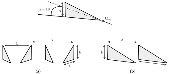
Figure 1.
Schemes of two main configurations. (a) Counter rotating VGs Configuration and (b) Co-rotating VGs Configurations of Vortex Generators.
In Figure 1, is the free stream velocity of the oncoming flow, and is the height and the length of the VG in the chord direction. The distance between two devices in the co-rotating and counter-rotating VG configuration is represented by λ and L, respectively, defining the distance between two devices in the trailing edge in the counter-rotating configuration.
The shape of the vortex generator and the location on the airfoil have a great impact on the flow control. Regarding the shape, extensive studies have been carried out with a triangular-shaped VG in order to determine its boundary-layer separation control effectiveness (see Lin [21] and Gad-el-Hak et al. [28]). Moreover, Zhang et al. [29] studied the effects of semi-delta VG on the aerodynamic performance of airfoils of thick wind turbines. Hansen et al. [30] presented an engineering model to calculate the generated vortex strength of rectangular and triangular VGs. In order to obtain the best solution for each case, parametric studies are necessary (see Jirasek [25]). Usually, these studies are conducted by means of fully meshed numerical simulations, which are very computationally demanding due to the high number of cells required to mesh the VG (see Fernandez-Gamiz et al. [31]).
A new source term model was settled by Bender et al. [32], called the BAY model, based on the Joukowski lift theorem and the thin airfoil theory, which uses forces to obtain a solution. Vane-type vortex generators were used for simulation by the finite volume Navier–Stokes code, while ignoring the condition to totally define the geometry in the mesh. For calibration, an analysis was conducted and the results achieved by this source term model were compared with those obtained for a fully meshed VG, as done by Errasti et al. [3]. Eventually, the BAY model for different flows with vane-type vortex generators was successfully evaluated by Dudek [33], changing the landscape of simulation of this type of aerodynamic element, enabling much faster analysis. Recently, an updated version called the jBAY model was developed and published by Jirasek [25]. This new version was based on the previous BAY model of Bender et al. [32], for which the technique used for flow simulation was more suitable.
The main objective of the current study was to implement a triangular vane-type vortex generator on a DU97W300 based on the jBAY source term model. This airfoil is part of the reference 5 MW wind turbine developed by NREL presented in Jonkman et al. [34]. Figure 2a represents the airfoil outline and Figure 2b the position of the airfoil on the blade. The aerodynamic performance of the airfoil is defined in the current study by the lift-to-drag ratio, and it was evaluated with and without a VG. Additionally, vortex trajectory, vortex decay, wall shear stress parameter, pressure coefficient distribution along the airfoil surface, and vortex visualization downstream of the VG were studied. The main advantage of the jBAY to model a triangular VG compared with the fully meshed model is that it is easy to implement, since no geometry of the VG is required. Additionally, this method is very flexible in case the user wants to change the size or geometry. The results obtained from this study provide specific information about VG performance by using the jBAY source term model.
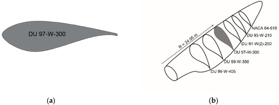
Figure 2.
(a) DU 97W300 airfoil; (b) sketch of blade airfoil distribution on NREL 5 MW blade.
The paper is structured as follows: Section 1 provides background information about the application of flow control devices in wind turbines and, in particular, the implementation of vortex generators. Section 2 gives a detailed description of the numerical model defined by means of computational fluid dynamics (CFD), while the results obtained and the effects on the airfoil aerodynamic performance are discussed in Section 3. Finally, Section 4 presents the more noteworthy conclusions obtained in the present study.
2. Materials and Methods
2.1. jBAY Model
Computational fluid dynamics (CFD) is the most common method used to simulate airflow and estimate airfoil efficiency. The combination of this tool and experiments in wind tunnels can be considered as a reliable method to conduct any parametric flow study. However, the fully meshed numerical simulations of VGs are very computationally demanding to carry out due to the high number of cells necessary to capture the VG effects.
In the current work, the jBAY source term model presented by Jirasek [25] and based on the BAY model developed by Bender et al. [32] was implemented in the commercial CFD code STAR CCM+® [35]. The BAY model was modeled to simulate vane-type vortex generators in finite volume Navier–Stokes codes and allows substituting the VG geometry by a subdomain of similar geometry at the same location. Then, a body force distribution normal to the local flow is applied to simulate the effect of the vane (see Figure 3). The normal force represented by Equation (1) is introduced as in Figure 3b. This normal force simulates the force generated by the VG without having to design and mesh it (see Fernandez-Gamiz et al. [36]). The force for each cell in the VG domain is calculated with Equation (1):
where is the force of the corresponding single cell; is a relaxation factor, which, according to Jirasek [25], usually has a value near 10; is the local density; is the local velocity; is a unit factor defined as (normal and tangential vectors to the VG); is the area of VG; is the volume of a single cell; and is the total volume of grid cells where the model is applied (see Errasti et al. [3]).
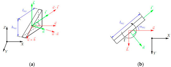
Figure 3.
View of forces on a triangular vortex generator (VG): (a) side view and (b) top view.
For this work, the forces, instead of applying them in all the subdomain cells as specified by BAY model, have been applied in those cells that represent the VG, as shown in Figure 4.
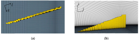
Figure 4.
Cells corresponding to the VG device where body forces are applied: (a) top view and (b) side view.
2.2. Computational Domain and VG Setup
The computational model is a DU97W300 with 0.65 m chord length (c) and 0.0175 m span length. A single VG was set up instead of a pair, with the assumption that the flow created behind the VG is symmetric. This strategy could contribute to reducing the computational time.
An O-shape computational domain was defined with a radius of 30 times the airfoil chord length. A symmetry boundary condition was implemented for the front and back sides and a nonslip wall boundary condition for the airfoil. A free stream condition was determined for the far-field domain. The domain was discretized by a structured mesh with a total of 6.64 million cells. Mesh refinement was defined in the region close to the leading and trailing edge, as well as at the VG position area, with a mesh growth rate of 1.1.
The configuration of the main VG variables in the airfoil is described in Figure 5. Table 1 shows the values of geometric parameters employed in this case. The VG was positioned at 30% of the chord length from the leading edge of the airfoil, .
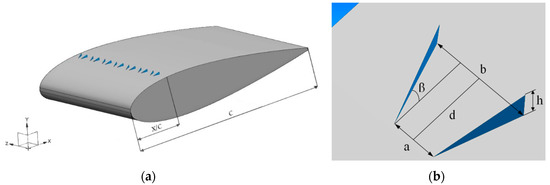
Figure 5.
Airfoil equipped with vortex generators (VGs): (a) row of vane-type VGs; (b) detailed view of VG pair with geometric dimensions.

Table 1.
Geometric measures of VG.
2.3. Numerical Models
Two numerical models were set up for the numerical simulations in the current work. In an incompressible and steady flow, the k-ω shear stress transport (SST) model of Menter [37] was used with the Reynolds-averaged Navier–Stokes (RANS) method to get a solution for cases where the angle of attack (AoA) is lower than 12°. However, according to Zhong et al. [38], the simplification of turbulence in the RANS method increases the inaccuracy of CFD, especially for phenomena directly related to turbulence. For this reason, at higher AoAs where the clean airfoil would be in a stall situation, Detached eddy simulation (DES) was set up. For instance, Meana-Fernandez et al. [39] determined that the results obtained in a DU-06-W-200 airfoil by the use of DES predicted the aerodynamic forces with good accuracy and provided more realistic flow patterns. This model combines features of the standard Spalart–Allmaras RANS model in boundary layers and large eddy simulation in unsteady separated regions (see Guo et al. [40]). The solution was considered to be converged with a three-order-of-magnitude drop in the numerical residuals.
One of the most important variables to define in a DES simulation is the Courant number (C). It depends on cell size , defined time steps , and flow velocity as shown in Equation (2). Briefly, this number indicates how a particle travels from one cell to an adjacent cell in a time step. If the Courant number is lower than or equal to 1, a flow particle will move from one cell to another in one time step; if the Courant number is bigger than 1, particles will move two or more cells in one time step. A Courant value of 20 was used in all unsteady cases studied, with a time step of 10−5.
In this study, the Reynolds number is × , based on airfoil chord length c = 0.65 m; × is the kinematic viscosity; and the free stream velocity is = 46.52 m/s (see Equation (3)):
3. Results
In the current study, the effects of VG implementation on an aerodynamic airfoil was investigated, with the following aerodynamic properties: lift and drag coefficients, vortex trajectory, vortex decay and wall shear stress, pressure coefficient distribution along the airfoil surface, and vortex visualization downstream of the VG for different angles of attack.
3.1. Lift and Drag Coefficients
According to Sørensen et al. [41], Fernandez-Gamiz et al. [42], and Timmer et al. [8], placing the VG over an airfoil results in a higher lift coefficient and a slight increase of residual drag. In all cases, this device allows the airfoil to be in steady state for larger AoAs than without it, getting higher lift values above all at stall angles of the clean airfoil. The lift and drag coefficients of the airfoil can be calculated with Equation (4):
where are the lift and drag coefficients, respectively; and are the force vectors on the surface face; , and are the reference density, velocity, and airfoil area, respectively; and is the specified direction vector depending on each force. The pressure force vector on a surface is computed by means of Equation (5):
where is the face static pressure; is the reference pressure; and is the face area vector. The shear force on surface face can be computed by Equation (6):
where is the stress tensor.
The analyzed angles of attack (AoAs) are in the range between 0 and 20°. The lift coefficients increase linearly until stall angles. These stall angles are located around 12° in the case of clean airfoil, according to Timmer et al. [8], and around 18–20° in the case of airfoil with VG according to the study by Gao et al. [22]. At those angles, effects related to flow separation appear and it begins to be affected by a worse lift coefficient, as shown in Figure 6a. The higher lift value appears just before the stall point, and it is greater in both value and AoA when using VGs. With the aim of validating the numerical results, they were compared with those of Gao et al. [22] in lift and drag coefficients and with the experimental data in the clean airfoil case [8]. Some differences are noted in the clean case between the numerical and experimental data at the beginning of stalling angles. Usually, CFD overestimates the lift coefficient at high AoAs (see the study by Li et al. [43]). Moreover, Raffel et al. [44] found some differences in light-stall situation between CFD and experimental data. Figure 6b shows the exponential increase of drag coefficient that arises beyond the stall angle.
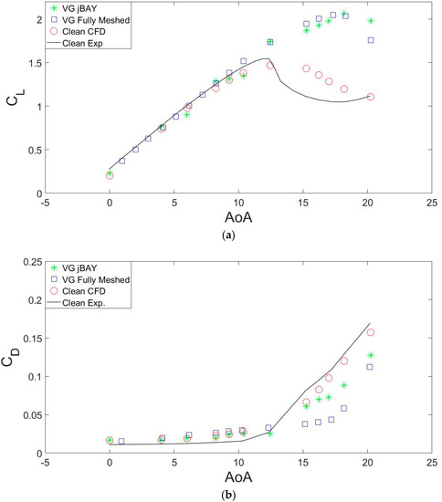
Figure 6.
Comparison for DU97W300 and Re = data of (a) lift coefficient and (b) drag coefficient between experimental and computational fluid dynamics (CFD) data.
3.2. Vortex Trajectory and Decay
The study performed in this work on peak vorticity in the VG was divided into two parts, investigating the values obtained for AoA in each case. The first part was focused on analyzing the path following peak vorticity values, whether horizontally or vertically. The second part studied the decay of peak vorticity values due to their distance in each moment from the VG device.
As concluded by Zhen et al. [45], vortices can be assumed as circular and it is in their center where the maximum peak value appears. Thanks to this peak localization, it is possible to determine the vortex path of each AoA downstream of the VG. The path of peak values is an important parameter to reach a more complete characterization of the created vortex and optimize the VG device. Even though several simulations and studies were done around this characterization and the detection of these peak values proved to be critical, Fernandez-Gamiz et al. [42] addressed successfully the characterization of the vortex path.
Meanwhile, in the case of a flat plane with VG devices, the vortex vertical path does not change its trajectory and is usually horizontal (see Ibarra-Udaeta et al. [46]). In the case of an airfoil profile, it was concluded that the vortex tends to follow parallel to the wall. This behavior of the vortex was concluded in Errasti et al. [3], where a VG device was set up on a flat plate and before going down a linear ramp. In this study, the vortex tended to continue the bottom wall path going down the ramp. The simulations performed for this purpose in the current work show that the generated vortex axes had similar vertical behavior in the first 20 mm after VG at all AoAs. From that distance onwards, the vortex vertical path slightly evolves in different ways, decaying faster at higher AoAs due to the length of the vortex, which is shorter at higher AoAs. Near stall state, the generated vortex in the boundary layer tends to separate from the surface of the airfoil, spreading in turbulent wakes that introduce major fluctuations in forces and increase the deviations of drag and lift coefficients. Thanks to VG devices, the boundary layer gets attached to the wall for larger degrees, but gets worse attitude at higher AoAs until a stall point is detected at 20°. The vertical trajectories can be seen in Figure 7, where the black line represents the airfoil surface.
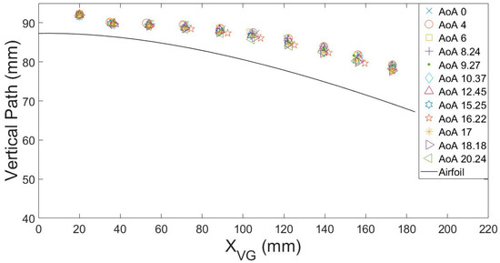
Figure 7.
Comparison of vertical peak vorticity paths for different angles of attack (AoAs).
As concluded in Ibarra-Udaeta et al. [46], the vortex peak path tends to deviate laterally in the direction marked by the device. In Figure 8 the lateral displacement can be noticed, which has a similar deviation for all AoAs in steady angles and stall angles, but is less displaced at high degrees. The trend of its deviation is higher at first distances in all cases, with a decay of deviation at 80 mm from the device. At 160 mm onwards, it is possible to see how the vortices at the highest AoA tend to go back to the device zero coordinate.
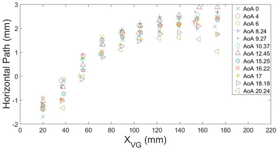
Figure 8.
Comparison of horizontal peak vorticity paths for different AoAs.
Vortex decay is a well-studied parameter that consists of the strength force loss of a vortex. In a study by Martínez-Filgueira et al. [6], the peak decay was analyzed over a flat plate. In that study, the decay development was exponential; the further it was from the device, the smaller the peak. In this study, values of the peak vorticity for every AoA in relation to the range toward VG are shown in Figure 9. It can be observed that the value varies for each angle, with different behavior between steady and stall angles in the near wake behind the VG. Higher peak vorticity values correspond to steady degrees, decreasing at higher AoAs. After the first 40 mm, the value of vorticity starts converging, with a similar value until the last 175 mm from the device, where it is less than 5000 s–1, and always lower for higher AoA.
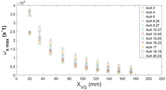
Figure 9.
Comparison of vortex decay at different chord positions for all angles of attack (AoAs).
3.3. Wall Shear Stress
Figure 10 shows the wall shear stress distribution along the first distances from the VG. The measurements were taken in a chordwise parallel line passing from the device trailing edge to 175 mm downstream. The results obtained agree with those obtained by Godard and Stanislas [24]. As in that case, the implementation of VGs increased the wall shear stress values downward in comparison with the clean airfoil.
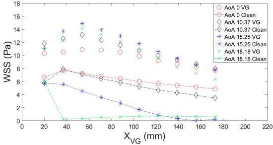
Figure 10.
Wall shear stress values for different angles of attack (AoAs).
In the cases with a VG set up over the airfoil, all plots show an increasing trend up to 54 mm downstream from the leading edge of the VG device. From this point onward, the values decay gradually up to a value between 42% and 70% at the last 173 mm from the VG (at higher AoAs, the difference between maximum and minimum is smaller). A maximum wall shear stress value of 14.86 is observed with an AoA of 15.25°.
In the case of the clean airfoil, two simulation types were evaluated: steady simulations at AoAs lower than 12.25° and DES based simulations at higher degrees. On the one hand, steady clean airfoil simulations present a maximum value closer to the device position than flow-controlled simulations, at 37 mm. From this point onward, the wall shear stress value starts decaying gradually. All steady simulations performed with the clean airfoil show a similar decaying gradient, with higher values at lower AoAs. On the other hand, the stall simulations present a maximum value at the first sampling point 20 mm from the VG leading edge and a subsequent decay until values reach next to zero. From this point onward, the wall shear stress values present a small increase that tends to be more stable. At higher AoAs, the distance of the null wall shear stress value from the VG device is closer.
3.4. Pressure Coefficient Distribution
Figure 11 shows the pressure distributions on the clean DU97W300 airfoil and the airfoil with VG at 0°, 4°, 6°, 10.27°, 15.25°, and 18.18° AoA. The airfoil profile and VG are illustrated with black lines. The difference between values at the pressure side and suction side represents the capacity to generate lift. The VG implementation barely affects the Cp distribution at low AoAs between the clean and flow-controlled airfoil. However, the increment in the pressure coefficient due to VG implementation is very noticeable at high angles of attack. It is from 12° onward where the device demonstrates high performance capacity. It is noteworthy that there exists a cut value in the suction side case due to the presence of the VG.
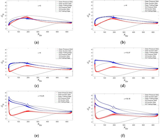
Figure 11.
Comparison for DU97W300 and Re = data of pressure coefficient at (a) 0°, (b) 4°, (c) 6°, (d) 10.37°, (e) 15.25°, and (f) 18.18° AoA.
3.5. Vortex Vizualization
Figure 12 illustrates the axial velocity fields for a qualitative comparison between six angles, AoA = 0°, 4°, 6°, 10.37°, 15.25°, and 18.18°. These snapshots were taken at the plane position five device heights downstream of the VG. According to Urkiola et al. [47], at that position the vortex is totally developed, and this shows how the vortex shape varies with the angle of attack. As a qualitative observation, it denotes that the size of the vortex increases with the AoA. The effect of the VG device is lower at small AoAs in comparison with higher angles. This is in agreement with the results presented in Figure 11 about the pressure distribution along the airfoil.
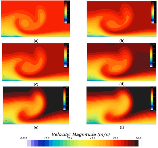
Figure 12.
Axial velocity fields at angles of attack of (a) 0°, (b) 4°, (c) 6°, (d) 10.37°, (e) 15.25°, and (f) 18.18° measured in a spanwise plane placed five device heights downstream of the VG.
4. Conclusions
The aerodynamic efficiency and vortex generated downstream of a delta VG device were investigated in this study. The geometry of the VG device is a semi-delta shape with a β = 18° incidence inclination, 5 mm height, and 17 mm length, and it was modelled by the so-called jBAY source term model. The distance between two devices is 10 mm measured from the leading edge and 20 mm from the trailing edge. The device was placed at in a DU97W300 airfoil of 0.65 m of chord. Computational simulations for this purpose were performed with a Reynolds number Re = and free stream velocity = 46.52 m/s using the DES method. The main conclusions are as follows: First, setting up a VG device is an efficient way to improve the lift coefficient of the DU97W300 airfoil in spite of the residual drag increment due to shear forces on the suction side. The jBAY model could be a key tool for parametric studies to find the optimal sizes and configurations of vane-type VGs. In addition, the vertical vortex trajectory is conditioned by the wall. The vortex will tend to adhere to the airfoil suction side for more angles of attack (AoAs), delaying the stall situation and improving the lift coefficient at those degrees. It allows improvement of the aerodynamic performance of the airfoil. Furthermore, from the results obtained it can be concluded that the vortex peak decay has a similar downing gradient at any AoA, but with higher values at lower AoAs. Another remarkable fact is the difference between the first values of peak vorticity, which have a clear difference between AoA = 12.45° and AoA = 15.25°. It is in this degree range where the clean airfoil starts entering the stall situation. Furthermore, on the one hand, it is clear that the VG device increases the wall shear stress, which leads to a slight increment of the overall drag force at those AoAs where the clean airfoil would be in a stall regime, due to the circulation generated by the VG. On the other hand, implementing the VG has a noticeable effect on the increment of the pressure coefficient of the DU97W300 airfoil from an AoA of 12° onward. At low AoAs, no clear difference exists between the Cp distribution on the clean and flow-controlled airfoils. Finally, it can be observed that the size of the vortex generated by implementing the VG increases with increasing angles of attack.
Author Contributions
S.C., P.M.-F., A.U.-U., and U.F.-G. developed and realized the CFD simulations. I.A., A.U.-U., S.C., and I.I.-U. curated the data and prepared the original draft. I.I.-U. and U.F.-G. handled the funding acquisition. All authors have read and agreed to the published version of the manuscript.
Funding
The authors are grateful to the government of the Basque Country and the University of the Basque Country UPV/EHU through the SAIOTEK (S-PE11UN112) and EHU12/26 research programs, respectively.
Acknowledgments
The authors are thankful for the technical and human support provided by SGIker of UPV/EHU.
Conflicts of Interest
The authors declare no conflict of interest.
Nomenclature
| Definition | Unit | |
| CFD | Computational fluid dynamics | |
| DES | Detached eddy simulation | |
| VG | Vortex generator | |
| RANS | Reynolds-averaged Navier–Stokes | |
| SST | Shear stress transport | |
| β | Vane incident angle | deg |
| Δt | Time step | s |
| Δx | Cell size | m |
| λ | Distance between two devices in co-rotating VG configuration Distance between pairs in counter-rotating VG configuration | mm |
| Local density | kg/m3 | |
| ω x max | Peak vorticity | s−1 |
| AoA | Angle of attack | deg |
| c | Airfoil chord length | m |
| C | Courant number | |
| CD | Drag coefficient | |
| CL | Lift coefficient | |
| CP | Pressure coefficient | |
| Relaxation factor | ||
| h | Height of vortex generator | mm |
| l | Length of vortex generator | mm |
| L | Distance between two devices in trailing edge in counter-rotating configuration | mm |
| Re | Reynolds number | |
| Area of vortex generator | m2 | |
| Free stream velocity | m/s | |
| WSS | Wall shear stress | Pa |
| XVG | VG position from airfoil leading edge | mm |
References
- Aramendia, I.; Fernandez-Gamiz, U.; Antonio Ramos-Hernanz, J.; Sancho, J.; Manuel Lopez-Guede, J.; Zulueta, E. Flow Control Devices for Wind Turbines. Energy Harvest. Energy Effic. Technol. Methods Appl. 2017, 37, 629–655. [Google Scholar] [CrossRef]
- Houghton, T.; Bell, K.; Doquet, M. Offshore transmission for wind: Comparing the economic benefits of different offshore network configurations. Renew. Energy 2016, 94, 268–279. [Google Scholar] [CrossRef]
- Errasti, I.; Fernandez-Gamiz, U.; Martinez-Filgueira, P.; Blanco, J.M. Source term modelling of vane-type vortex generators under adverse pressure gradient in OpenFOAM. Energies 2019, 12, 605. [Google Scholar] [CrossRef]
- Baldacchino, D.; Manolesos, M.; Ferreira, C.; Salcedo, A.G.; Aparicio, M.; Chaviaropoulos, T.; Diakakis, K.; Florentie, L.; García, N.R.; Papadakis, G. Experimental benchmark and code validation for airfoils equipped with passive vortex generators. J. Phys. Conf. Ser. 2016, 753, 022002. [Google Scholar] [CrossRef]
- Fernandez-Gamiz, U.; Zulueta, E.; Boyano, A.; Ramos-Hernanz, J.A.; Manuel Lopez-Guede, J. Microtab Design and Implementation on a 5 MW Wind Turbine. Appl. Sci. 2017, 7, 536. [Google Scholar] [CrossRef]
- Martinez-Filgueira, P.; Fernandez-Gamiz, U.; Zulueta, E.; Errasti, I.; Fernandez-Gauna, B. Parametric study of low-profile vortex generators. Int. J. Hydrogen Energy 2017, 42, 17700–17712. [Google Scholar] [CrossRef]
- Johnson, S.J.; Baker, J.P.; van Dam, C.P.; Berg, D. An overview of active load control techniques for wind turbines with an emphasis on microtabs. Wind Energy 2010, 13, 239–253. [Google Scholar] [CrossRef]
- Van Rooij, R.; Timmer, W. Roughness sensitivity considerations for thick rotor blade airfoils. J. Sol. Energy Eng. 2003, 125, 468–478. [Google Scholar] [CrossRef]
- United Aircraft Corporation, Research Department; Taylor, H. Summary Report on Vortex Generators; United Aircraft Corporation, Research Department: East Hartford, CT, USA, 1950. [Google Scholar]
- Bragg, M.; Gregorek, G. Experimental study of airfoil performance with vortex generators. J. Aircr. 1987, 24, 305–309. [Google Scholar] [CrossRef]
- Schepers, G. Avatar: Advanced aerodynamic tools of large rotors. In Proceedings of the 33rd Wind Energy Symposium, Kissimmee, FL, USA, 5–9 January 2015; p. 0497. [Google Scholar]
- Zahle, F.; Tibaldi, C.; Verelst, D.R.; Bitche, R.; Bak, C. Aero-elastic optimization of a 10 MW wind turbine. In Proceedings of the 33rd Wind Energy Symposium, Kissimmee, FL, USA, 5–9 January 2015; p. 0491. [Google Scholar]
- Fernandez-Gamiz, U.; Errasti, I.; Gutierrez-Amo, R.; Boyano, A.; Barambones, O. Computational modelling of rectangular sub-boundary layer vortex generators. Appl. Sci. 2018, 8, 138. [Google Scholar] [CrossRef]
- Zaman, K.; Reeder, M.; Samimy, M. Control of an Axisymmetrical Jet using Vortex Generators. Phys. Fluids 1994, 6, 778–793. [Google Scholar] [CrossRef]
- Astolfi, D.; Castellani, F.; Terzi, L. Wind Turbine Power Curve Upgrades. Energies 2018, 11, 1300. [Google Scholar] [CrossRef]
- Terzi, L.; Lombardi, A.; Castellani, F.; Astolfi, D. Innovative methods for wind turbine power curve upgrade assessment. In Proceedings of the Windeurope Conference 2018 within the Global Wind Summit, Hamburg, Germany, 25–28 September 2018; Volume 1102. [Google Scholar] [CrossRef]
- Florentie, L.; Hulshoff, S.J.; van Zuijlen, A.H. Adjoint-based optimization of a source-term representation of vortex generators. Comput. Fluids 2018, 162, 139–151. [Google Scholar] [CrossRef]
- Øye, S. The effect of vortex generators on the performance of the ELKRAFT 1000 kw turbine. In Proceedings of the 9th IEA Symposium on Aerodynamics of Wind Turbines, Stockholm, Sweden, 11–12 December 1995. ISSN 0590-8809. [Google Scholar]
- Miller, G. Comparative performance tests on the Mod-2, 2.5-MW wind turbine with and without vortex generators. In Proceedings of the DOE/NASA Workshop on Horizontal Axis Wind Turbine Technology, Cleveland, OH, USA, 1 May 1995. [Google Scholar]
- Schubauer, G.B.; Spangenberg, W.G. Forced mixing in boundary layers. J. Fluid Mech. 1960, 8, 10–32. [Google Scholar] [CrossRef]
- Lin, J. Review of research on low-profile vortex generators to control boundary-layer separation. Prog. Aerospace Sci. 2002, 38, 389–420. [Google Scholar] [CrossRef]
- Gao, L.; Zhang, H.; Liu, Y.; Han, S. Effects of vortex generators on a blunt trailing-edge airfoil for wind turbines. Renew. Energy 2015, 76, 303–311. [Google Scholar] [CrossRef]
- Betterton, J.; Hackett, K.; Ashill, P.; Wilson, M.; Woodcock, I.; Tilman, C.; Langan, K. Laser doppler anemometry investigation on sub boundary layer vortex generators for flow control. In Proceedings of the 10th Symposium on Application of Laser Techniques to Fluid Mechanics, Lisbon, Portugal, 10–13 July 2000; pp. 10–12. [Google Scholar]
- Godard, G.; Stanislas, M. Control of a decelerating boundary layer. Part 1: Optimization of passive vortex generators. Aerospace Sci. Technol. 2006, 10, 181–191. [Google Scholar] [CrossRef]
- Jirasek, A. Vortex-generator model and its application to flow control. J. Aircr. 2005, 42, 1486–1491. [Google Scholar] [CrossRef]
- Bray, T.P. A Parametric Study of Vane and Air-Jet Vortex Generators. Ph.D. Thesis, College of Aeronautics, Cranfield University, Bedford, UK, 1998. [Google Scholar]
- Bur, R.; Coponet, D.; Carpels, Y. Separation control by vortex generator devices in a transonic channel flow. Shock Waves 2009, 19, 521. [Google Scholar] [CrossRef]
- Gad-elHak, M.; Bushnell, D. Separation Control—Review. J. Fluids Eng.-Trans. ASME 1991, 113, 5–30. [Google Scholar] [CrossRef]
- Zhang, L.; Li, X.; Yang, K.; Xue, D. Effects of vortex generators on aerodynamic performance of thick wind turbine airfoils. J. Wind Eng. Ind. Aerodyn 2016, 156, 84–92. [Google Scholar] [CrossRef]
- Hansen, M.O.L.; Charalampous, A.; Foucaut, J.; Cuvier, C.; Velte, C.M. Validation of a Model for Estimating the Strength of a Vortex Created from the Bound Circulation of a Vortex Generator. Energies 2019, 12, 2781. [Google Scholar] [CrossRef]
- Fernandez-Gamiz, U.; Marika Velte, C.; Réthoré, P.; Sørensen, N.N.; Egusquiza, E. Testing of self-similarity and helical symmetry in vortex generator flow simulations. Wind Energy 2016, 19, 1043–1052. [Google Scholar] [CrossRef]
- Bender, E.; Anderson, B.; Yagle, P. Vortex generator modeling for Navier-Stokes codes. In Proceedings of the Third ASME/JSME Joint Fluids Engineering Conference, California, USA, 18–23 July 1999; pp. FEDSM99–FEDSM6919. [Google Scholar]
- Dudek, J.C. Modeling vortex generators in a Navier-Stokes code. AIAA J. 2011, 49, 748–759. [Google Scholar] [CrossRef]
- Jonkman, J.; Butterfield, S.; Musial, W.; Scott, G. Definition of A 5-MW Reference Wind Turbine for Offshore System Development, Technical Report; National Renewable Energy Laboratory (U.S.): Golden, CO, USA, 2009. [CrossRef]
- Siemens STAR CCM+ Version 13.02.011. Available online: http://mdx.plm.automation.siemens.com/ (accessed on 9 April 2020).
- Fernandez, U.; Réthoré, P.-E.; Sørensen, N.N.; Velte, C.M.; Zahle, F.; Egusquiza, E. Comparison of four different models of vortex generators. In Proceedings of the EWEA 2012—European Wind Energy Conference & Exhibition European Wind Energy Association (EWEA), Copenhagen, Denmark, 16–19 March 2012; pp. 1–15. [Google Scholar]
- Menter, F. Zonal two equation kw turbulence models for aerodynamic flows. In Proceedings of the 23rd Fluid Dynamics, Plasmadynamics, and Lasers Conference, Orlando, FL, USA, 6–9 July 1993; p. 2906. [Google Scholar]
- Zhong, W.; Tang, H.; Wang, T.; Zhu, C. Accurate RANS Simulation of Wind Turbine Stall by Turbulence Coefficient Calibration. Appl. Sci. 2018, 8, 1444. [Google Scholar] [CrossRef]
- Meana-Fernandez, A.; Fernandez Oro, J.M.; Arguelles Diaz, K.M.; Velarde-Suarez, S. Turbulence-Model Comparison for Aerodynamic-Performance Prediction of a Typical Vertical-Axis Wind-Turbine Airfoil. Energies 2019, 12, 488. [Google Scholar] [CrossRef]
- Guo, C.; Guo, H.; Hu, J.; Song, K.; Zhang, W.; Wang, W. Large Eddy Simulation of Flow over Wavy Cylinders with Different Twisted Angles at a Subcritical Reynolds Number. J. Mar. Sci. Eng. 2019, 7, 227. [Google Scholar] [CrossRef]
- Sorensen, N.N.; Zahle, F.; Bak, C.; Vronsky, T. Prediction of the Effect of Vortex Generators on Airfoil Performance. In Science of Making Torque from Wind 2014 (Torque 2014); Journal of Physics: Conference Series; IOP Publishing: Copenhagen, Denmark, 2014; Volume 524. [Google Scholar] [CrossRef]
- Fernandez-Gamiz, U.; Zamorano, G.; Zulueta, E. Computational study of the vortex path variation with the VG height. In Science of Making Torque from Wind 2014 (Torque 2014); IOP Publishing: Copenhagen, Denmark, 2014; Volume 524. [Google Scholar] [CrossRef]
- Li, S.; Zhang, L.; Yang, K.; Xu, J.; Li, X. Aerodynamic Performance of Wind Turbine Airfoil DU 91-W2-250 under Dynamic Stall. Appl. Sci. 2018, 8, 1111. [Google Scholar] [CrossRef]
- Raffel, M.; Favier, D.; Berton, E.; Rondot, C.; Nsimba, M.; Geissler, W. Micro-PIV and ELDV wind tunnel investigations of the laminar separation bubble above a helicopter blade tip. Meas. Sci. Technol. 2006, 17, 1652–1658. [Google Scholar] [CrossRef]
- Zhen, T.K.; Zubair, M.; Ahmad, K.A. Experimental and Numerical Investigation of the Effects of Passive Vortex Generators on Aludra UAV Performance. Chin. J. Aeronaut. 2011, 24, 577–583. [Google Scholar] [CrossRef]
- Ibarra-Udaeta, I.; Errasti, I.; Fernandez-Gamiz, U.; Zulueta, E.; Sancho, J. Computational Characterization of a Rectangular Vortex Generator on a Flat Plate for Different Vane Heights and Angles. Appl. Sci. 2019, 9, 995. [Google Scholar] [CrossRef]
- Urkiola, A.; Fernandez-Gamiz, U.; Errasti, I.; Zulueta, E. Computational characterization of the vortex generated by a Vortex Generator on a flat plate for different vane angles. Aerospace Sci. Technol. 2017, 65, 18–25. [Google Scholar] [CrossRef]
© 2020 by the authors. Licensee MDPI, Basel, Switzerland. This article is an open access article distributed under the terms and conditions of the Creative Commons Attribution (CC BY) license (http://creativecommons.org/licenses/by/4.0/).